Savitzky-Golay Least-Squares Polynomial Filters in ECG Signal Processing S Hargittai Innomed Medical Inc., Budapest, Hungary
Abstract
2.
The Savitzky-Golay(SG) filters are widely used for smoothing and differentiation in many fields namely in elastography, EEG and magnetocardiogram signal processing and mainly in absorption spectroscopy. Despite their exceptional features they were rarely used so far in the ECG signal processing. The aim of this paper is the investigation of their properties in detail from the ECG signal processing aspect. There were considered smoothing and differentiation filters approximating polynomials of zero to fourth order with 3 – 25-point lengths. The filtering effect and the retaining of small details of signal are opposite requirements and depend on the length and the order of applied polynomial. Taking into consideration 500 Hz sampling rate, size of smallest relevant ECG and requirements of approximating peaks and inflections in ECG signal processing, the best choice of use is the quartic smoothing and differentiation filters with 17-point length.
1.
First, theoretical analysis was performed in the time and frequency domain, and then the SG filters were applied to artificial and real ECG records. Analytical ECG records from the EN 60601-2-51 standard are used as artificial ECG, and records from the CSE multi-lead database are used as real ECG. All used signals had 500 Hz sampling rate.
2.1. Investigating SG smoothing filters in the time domain Since SG filters have been derived from the field of numerical analysis they were first investigated in the time domain. Consideration was carried out by the next properties: • reproducing of polynomials; • noise amplification, noise reduction; • preserving small details, such as small q- and rwaves. Let us fit the signal with polynomial. Assuming the derivatives of degree higher than p to be zero, the Taylor polynomial is given by:
Introduction
The classical work of Savitzky and Golay [1] and the articles containing the corrected filter coefficients [2,3] have been cited by countless articles. The SG filters are mainly used for smoothing and differentiating data in absorption spectroscopy [1-4]. Recently they have appeared in strain calculation in ultrasound elastography [5], however, I have not found considerable references from the ECG field. The method is based on the following principle. 2m+1 equidistant points (-m, … 0, …, +m) obtained by sampling is assumed to represent samples of degree p polynomial additively corrupted by zero–mean measurement noise. The SG method estimates the value of the least-squares polynomial or its derivatives at point i = 0. There is no need to fit new polynomial again and again for the following points, this can be automatically performed by applying a convolution with constant coefficients. Such way a running least-squares polynomial fitting is performed automatically to samples. Filter coefficients evaluation is not the objective of this paper.
0276−6547/05 $20.00 © 2005 IEEE
Methods
∑
i k f (k ) (x ) , k! k =0 p
f (x + i ) =
(1)
After convolving the polynomial with the filter under consideration and rearranging the summations we get:
∑∑
i k f (k ) (x ) ci k! i = − m k =0
(2)
f (k ) (x ) i k ci k! i = − m
(3)
m
g (x + i ) =
∑ p
g (x + i ) =
k =0
p
∑( ) m
For reproducing the values and derivatives of the noise free polynomial of degree no higher than p the filter coefficients must be satisfied with the next equations: k =0 1 m k (4) i ci = 0 k = 1... p i =− m k>p ≠ 0 for the smoothing filter,
∑( )
763
Computers in Cardiology 2005;32:763−766.
0 − 1 i k ci = 0 i =− m ≠ 0
∑( ) m
k=0 k =1 k = 2... p
(5)
k>p for the filter of estimating first derivative, k = 0,1 0 2 m k=2 (6) i k ci = k = 3... p 0 i =− m ≠ 0 k>p for the filter of estimating second derivative. The error for the first polynomial, which is not correctly reproduced, is constant. Raising the degree of considered polynomial the error will be first and than second order and so on. Results of accomplished calculations for filter coefficients and tests corresponded with theory.
∑( )
Figure 2. EN 60601-2-51 ANE20000, lead V4+HF noise Table 1.
9 points 11 points 13 points 15 points 17 points 19 points 3 points 5 points 7 points
Noise EN60601-2-51, amplification RMS 107.9363 µV 2nd pol. 4th pol. 2nd pol. 4th pol. 0.26 0.41 44.61 56.48 0.21 0.33 38.58 51.84 0.17 0.27 33.73 46.02 0.15 0.23 26.63 43.56 0.13 0.21 21.41 40.12 0.12 0.18 20.45 35.35 0th 0th 0.33 52.39 0.20 38.75 0.14 28.70
Let us consider now the degree of preserving the small details of ECG signals, such as small q- and r-waves. Figure 1. Reproducing of 4th degree polynomial. Error is shown on the lower part. The central moments have taken the values according to equations (4–6). As an example the reproducing of 4th order polynomial is shown in Figure 1. Order of error is equal to what is expected. But the error is not noticeable without magnification. It is less than 1 % even by fitting with zero order polynomial. The 4th order polynomial fitting has zero error apart from the truncation error. The noise amplification in a filter is equal to the sum of the squares of the filter coefficients [6]. The calculated noise amplifications and the values for the high-frequency (HF) noise from standard are shown in Table 1. Figure 2 shows that the zero order smoothing filter (as a matter of fact it is a moving averaging filter) hardly rejects the HF noise.
Figure 3. EN 60601-2-51 ANE20000, lead aVL
764
have almost the same cut-off frequency. What are the differences between them? It can be said for the transfer function of the filters satisfied equation (4) that its derivative up to p order equal zero at ω = 0 [6]. The more order of polynomial that we have to fit in the time domain, the higher the tangency at ω = 0 in the frequency domain, consequently the functions are also flatter there. Another difference is that the main lobe of the transfer function comes down more rapidly as the order of polynomial increases. For this reason the frequency response of the smoothing filter using higher order polynomial is closer to the ideal LP filter.
Figures 3–5 show the results of applying the considered smoothing filters to ECG signals. Only one from the averaging filters - the filter with 3-point length can more or less follow the small waves. The behavior of the 2nd and 4th order smoothing filters was similar, but the 4th order filters were slightly better since they did not widen the small waves.
Figure 4. CSE MO1_014, lead V3
Figure 6. Smoothing filters The 5-point zero order, the 11-point second order and the 17-point fourth order least squares smoothing give the best overall performance for each order of polynomials. The two filters of higher order polynomial are much better than the moving averaging filter. The 17-point fourth order smoothing is better than the 11-point second order.
2.3.
Differentiation SG filters
For the ideal differentiation filter the following is true: d k x
Figure 5. CSE MO1_002, lead V1
F
2.2. Investigating SG smoothing filters in the frequency domain
dt
(t ) = ( jω )k F [x(t )]
k
(7)
Therefore it amplifies the HF noise much more than ECG signal having relatively lower frequencies. For this reason the low-pass digital differentiators (LPDD) are used in practice. LPDDs try to approximate the ideal differentiator as well as possible in the passband and to reject the frequencies that lie outside. For this reason their behavior at zero frequency is most important. From equations (5) and (6) it follows that the derivatives of the transfer function of SG differentiators
We have to wonder, whether the frequency point of view could explain the filters’ behavior considered above. As filter length and order of polynomials decreases, the main lobe of the transfer function is getting wider and consequently the cut-off frequency increases. On the right side of Figure 6 the frequency responses of the three best filters show considerable similarity; for example, they
765
are zero up to p order except the order of differentiation. In other words the SG differentiators using higher order polynomial better approximate the ideal differentiator at ω = 0. This can be considered in Figure 7.
filter coefficients can be easily obtained from tables or from explicit equations [1-3]; • perform running least-squares polynomial fitting applying simple convolution; • perform smoothing and differentiation simultaneously; • length and polynomial order can be chosen according to signal form and sampling rate; • possibility of using same order polynomials for obtaining different order derivatives during processing of the same signal. The filtering effect and the retaining of small signal details are opposite requirements and depend on the length and the order of the applied polynomial. Taking into consideration 500 Hz sampling rate, size of smallest relevant ECG waves (30 µV, 12 ms) and requirements of approximating peaks and inflections in ECG signal processing the best choice of use is the quartic smoothing and differentiation filters with 17-point lengths. •
Acknowledgements
Figure 7. First order differentiators
The author would like to thank István Horváth for his help with proofreading and making the poster presentation.
For differentiators the difference of performance is much bigger between the second and fourth order polynomial filters than for smoothing filters. The last ones are better having more accurate low-frequency behavior. On the right hand side of Figure 7 the ratio of calculated to the true answer [6] is shown for the applied filters. The ratio for the fourth order polynomial differentiators equals nearly one up to higher frequencies than for second order polynomial differentiators and comes down more rapidly.
3.
References [1] Savitzky A, Golay MJE. Smoothing and differentiation of data by simplified least squares procedures. Analytical Chemistry 1964;36;1627–1639. [2] Steiner J, Termonia Y, Deltour Y. Comments on smoothing and differentiation of data by simplified least squares procedure. Analytical Chemistry 1972;44;1906–1909. [3] Madden HH. Comments on the Savitzky-Golay convolution method for least-squares fit smoothing and differentiation of digital data. Analytical Chemistry 1978; 50;1383–1388. [4] Mark H, Workman JJr. Derivatives in spectroscopy, Part III – computing the derivative. Spectroscopy 2003 Dec;18.106-111. [1] Luo J, Bai J, He P, Ying K. Axial strain calculation using a low-pass digital differentiator in ultrasound elastography. IEEE Trans. Ultrason., Ferroelect.,Freq Contr 2004 September;51;1119–1127. [2] Hamming RW. Digital filters. Prentice-Hall International Editions; 1989.
Results
It can be stated that increasing the order of the applied polynomial and decreasing length of SG filters leads to the better preservation of the small details of QRS complex, while decreasing the rejection of undesirable noises. The use of the unnecessary high order polynomial with short length leads to overfitting, in other words the HF noise is also approximated. Reduction of peak amplitudes can be observed using either the low order polynomial with short length or high order polynomial with long length, but at the same time the lower order polynomial filters suppress the noises less. The SG differentiators using higher order polynomial fitting better approximate the ideal differentiator at low frequencies.
4.
Address for correspondence Sándor Hargittai Innomed Medical Inc. Szabó József utca 12. H-1146. Budapest Hungary E-Mail:
[email protected]
Discussion and conclusions
Advantages of using SG smoothing and differentiation filters are: • common theoretical background for developing smoothing and differentiation filters;
766