CAPABILITY OF SLUG FLOW MODEL FOR PREDICTION OF PRESSURE DROP IN GAS-LIQUID TWO-PHASE ‘ SLUG ’ FLOW Nay Zar Aunga, Triyogi Yuwonob Laboratory of Fluid Mechanics, Department of Mechanical Engineering, Institute Technology Sepuluh Nopember (ITS) Campus ITS, Sukolio, Surabaya 60111, Indonesia a:
[email protected] b:
[email protected]
Abstract Slug flow model is well known flow pattern dependent model for modeling two-phase slug flow. In this work, pressure drops in gas-liquid slug flow were predicted by using slug flow model and some existing empirical correlations (Lockhart-Martineli correlation and Friedel correlation). The predicted data are validated with experimental data of Henry Nasution (2000). The experiments were conducted in a 0.024 m (ID) vertical acyclic pipe with a variation of superficial liquid velocity from 0.14 m/s to 1.4 m/s and superficial gas velocity from 0.114 m/s to 2.68 m/s Henry Nasution (2000). The prediction capability of slug flow model was compared with that of chosen empirical correlations. The results showed that the slug flow model gives reliable predictions at low gas rates. In this work, predictions of slug flow model have error of about 30 % and it is weaker than Lockhart-Martineli correlation. At low gas and liquid velocities, slug flow model gave better perditions than other two correlations. Key words; Capability, Slug flow model, Pressure drop, gas-liquid two-phase slug flow
1. INTRODUCTION When gas and liquid flow in a pipe, they tend to distribute themselves in a variety of configurations. These distribution characteristics of the fluid–fluid interface are called flow patterns or flow regimes. In a vertical co-current gas-liquid flow, the most common flow patterns are bubbly flow, slug flow, chun flow, annular flow and mist flow and their physical configurations are shown in Fig.1 Slug flow is frequently encountered in gasliquid two-phase flow applications, such as, airlift pump, oil & gas transporting pipe lines, etc. Usually, it is an unfavorable flow pattern due to its unsteady nature, intermittency and high-pressure drop [Yehuda Taitel (1999)]. However, in airlift pump operation, the best efficiency was found to be in the slug and slug-churn flow regimes [Ahmed (2008)]. Any way, knowledge of slug flow characteristics is very necessary and reliable predictions of pressure drop in two-phase slug flow are very important. In two-phase flow applications, flow patterns are intimately interrelated to the transport phenomena such as heat, mass and momentum transfer. As a consequence, in two-phase flow, hydrodynamic phenomenon (pressure drop) is very capabilities for some flow patterns. For examples, Spedding (2006) recommended Duklar–Wicks– Cleveland, Beggs–Brill and Olujic correlations for stratified regimes and Friedel correlation for annular flow patterns. According to Thome (2001), in refrigerant flow, Muller-Steinhagen and Heck correlation was the best for annular flow and for the
dependent on flow pattern. Thus, existing (flow pattern independent) empirical correlation developed for pressure drop prediction are only of limited reliability and pressure drops predicted using existing empirical equations often differ by 50% or more [Thome (2007)]. Nowadays flow pattern based pressure drop models are also become widely used in prediction of two-phase flow pressure drops. Some attempts have been done on twophase flow pressure drop predictions by using existing empirical correlations. Spedding (2006) have predicted two-phase (gas-liquid) and three phase (gas-water-oil) pressure drop by using Lockhart–Martinelli correlation, Dukler–Wicks– Cleveland correlation, Beggs–Brill correlation, Friedel correlation, Beattie–Whalley correlation, Muller Steinhagan–Heck correlation, Olujic correlation. Thome (2001) has also has done the prediction of pressure drop in refrigerant (R-134a, R-123, R-402A, R-404A and R-502) two-phase flow by using previous correlations. Prediction of twophase pressure drop by any of the chosen correlations was not successful over all flow regimes Spedding (2006). They observed that some of these empirical correlations have good prediction cases of intermittent flow (slug, plug flow) and stratified-wavy flow, Grönnerud correlation was the most appropriate correlation. That is obvious that the pressure drops in two-phase flow are very dependent on the flow pattern formation and the appropriate models should be applied to obtain the reliable predictions.
1
Therefore, it is desirable to know if the flow pattern dependent pressure models can give reliable predictions. And also, no attempt has been done for prediction of two-phase flow pressure drop by using flow pattern dependent model and the existing correlations at the same time to compare their prediction capabilities. Therefore, the main objective of this work is to predict the pressure drop in gas-liquid slug flow by using slug flow model to know the capability of slug flow model in prediction of pressure drop in gas-liquid slug flow. The other objective is to compare the capability of slug flow model with that of existing empirical correlations (LockhartMartineli correlation, Grönnerud correlation).
(2) u b 0.54 gD cos 0.35 gD sin where D is the pipe diameter, g the acceleration of gravity and is the inclination angle measured from the horizontal. By taking mass conservation in one unit slug length, (3) U SL A l u u s A LS l S u Lf A Lf l f By taking mass conservation relative to slug transional velocity (ut) for one slug (4) (u t u Lf ) Lf u t u S LS When the liquid mass conservation law is applied to the slug unit, and no slip is assumed in the slug cylinder (i.e, um = uS) and having lf + lS = lu., it is possible to express the ratio of film and total slugunit length, lf/lu as follow. lf u LS (5) m lu u t LS Lf The liquid fraction of the total slug unit can be defined as l Lf l f C LS (6) L LS S lu 1 C The liquid fraction depends on two correlating parameters: the shedding parameter C (shedding parameter) and the liquid fraction in the slug body, LS . For knowing LS , the correlation
2. EXPERIMENTAL SETUP The experiments of pressure drop measurements were carried out using the apparatus as shown in Fig.2. A detailed description of the experimental setup can be seen in Henry Nasution (2000). The working fluids are air (at 1 atm and 20C) and water (at 27.6 C). In order to measure the pressure drop, two pressure taps which are connect with U type manometer were installed 1.4 m apart from each other on the test section. The test section is 0.024 m ID acrylic circular pipe. Different ‘slug’ flow conditions are created by varying gas velocities at constant liquid velocity and by varying liquid velocity at constant gas velocity. The flow rates of water and air are measured by using flow meter and rotameter respectively.
developed by Andreussi and Bendiksen (1998) on the basis of small-scale laboratory data is being used.
3. MATHEMATICAL SLUG FLOW MODEL Slug flow is one of the most complicated multiphase flows in pipeline. The analysis assumes identical slugs and the calculations are performed on a single typical slug unit. A schematic geometry of the system is shown in Fig.3. Slug flow can be divided into two regions; one region is called the film region and consists of liquid film at the bottom and gas packet at the top. The other region is called the slug region and consists of the slug body and gas bubbles in the body. The sum of the film region and the slug region is called the slug unit. The slug propagates at the translational velocity, u t which
u m 0 u m1 u m0 u m
LS
For u m u m1
For
1
u m u m1
(7)
where, um1 is bubble dispersed velocity and um0 is bubble recoalescing velocity. The um1 is can be defined with a fixed value of 1 m/s [Clayton T. Crowe (2006)] The bubble recoalescing velocity is
u m0
240 1 / 2 1 g E 0 1 sin 2 C 0 1 3 L
1/ 4
ub C 0 1 (8)
can be obtained from the expression proposed by Nicklin (1962) (1) u t (1 C) u m C0 u m u b where C is shedding factor and C0 is an empirical velocity distribution parameter that is approximately equal to the ratio of the maximum to the mean fully developed velocity profile. Nicklin (1962) proposed a value of C0 =1.2 for turbulent flow and C0 is about 2.0 for laminar flow. Laminar or turbulent can be checked with Re m = L D um/L .For bubble rise velocity ub, Bendiksen (1984) proposed the use of
gD 2 (9) 4 The following expressions are used for calculing actual velocities of liquid and gas in those regions: Lf u m (10) u Lf 1 C LS Lf where,
E0
Lf u Gf 1 C LS 1 Lf
2
u m
(11)
The ratio of the length of the slug body to l the length of the total slug unit, S , by using a lu correlation introduced by Heywood and Richardson (1979) lS L 0.1 for L > 0.1 (12) lu The frictional part of the pressure gradient for intermittent flow can be written as a sum of liquid film and slug body; P P 1 lf Ps dp Wf f Wb b dx S lS 0 A A A dz friction l u
4 AG (27) PG Pi Neglecting momentum pressure drop with an assumption steady state, the total pressure gradient is mentioned as; P l Pf u2 l dp Wb b f 2 f S S m S Wf A A lu D lu dz ( G G L L ) g sin (28) DG
4. TWO-PHASE FLOW PRESSRURE DROP EMPERICAL CORRECLATIONS Exiting empirical correlations are easy to implement and often they provide good accuracy in the range of the database which had been used in developing the corresponding correlation. Therefore empirical formulae are still useful and still being used in industrial applications. The Lockhart–Martinelli (Lockhart and Martinelli, 1949) correlation is perhaps the oldest available correlation for two-phase frictional pressure drop. However, because of its liquid fraction correlation, it is also applicable for vertical upward flow (dss, 2006) It was widely used in industries. It is very simple to apply. One of the most accurate twophase pressure drop correlations is said to be that of Friedel. It was obtained by using a large data base of two-phase drop measurements. It is also applicable to vertical upflow and to horizontal flow because the data bank was developed from horizontal and vertical flow measurements. Therefore, in this study, Lockhart –Martineli correlation and Friedel correlation were chosen to compare with capability of slug flow model. Detail descriptions of chosen correlations can be seen in Lockhart and Martinelli (1949) and Friedel (1979).
(13)
Wb f G
2 G u Gf 2
(14)
L u 2Lf (15) 2 To find the perimeters (Pf, Pb) occupied by liquid and gas, the following equations are used. sin Lf (16) 2 D Pf (17) 2 (18) Pb D PL (19) Pi sin( / 2) D Wf f L
Frictional pressure gradient for slug region can be mentioned as u2 dp 2 f S S m D dz friction ,slug
(20)
where the slug density is (21) S LSS (1 LS ) G All of required friction factors (fS, fL,fG) can be calculated from numbers (ReS, ReL, ReG ) using following expressions.
f 1 f
16 Re 3.48 4 log (2k / D
5. PROCEDURE OF PREDICTION
Re 2300
9.35 Re f
) Re > 2300
(22)
Fig.4 shows the flow chart which summarizes the calculation of pressure gradient for two-phase slug flow. All calculation will be served by using MATLAB programs. As a prerequisite, the required input parameters have to be determined as input data are shown in Table 1. The properties of fluids used in this work are shown in Table 2. 6. RESULTS AND DISCUSSION
The Reynolds numbers can be calculated with following expressions. (23) ReS D S u m / L
Figs. 5-6 show the comparisons of predicted pressure drop and experimental pressure drop for two-phase slug flow. Comparisons have been made in different conditions in which gas flow rate was varied at constant liquid flow rate and also liquid flow rate was varied at constant gas flow rate. By overviewing the results from this study, it was observed that the slug flow model predicted pressure drop with error of around 30 %. At low
(24) ReL D L L u Lf / L (25) ReG D G G u LG / G The hydraulic liquid diameter and hydraulic gas diameter are 4AL DL (26) PL
3
gas and liquid velocities, slug flow model can give good predictions with low error; it can be seen in Table 3 and 4. At USG = 0.114 m/s with variation USL (Fig. 6(a) and Table 4) slug flow model gave good prediction with an error of 12.349 % which is better than Lockhart-Martinelli correlation and Friedel correlation. The results showed that prediction capability of slug flow model is weaker than that of Lockhart-Martinelli correlation. In this work, Lockhart-Martineli correlation could predict slug flow pressure drop with average error of less than 20 % and it gives better predictions rather than other two prediction methods. Friedel correlation gave good predictions at high liquid velocities; it can be seen that in Table 3. The higher the liquid velocity, the lower prediction error Friedel correlation can give. But at high gas velocity (U SG = 2.68 m/s), it gave a high error of greater than 50 %. In this work, the slug flow model is combination of a set of fluid transport equations and submodels or closure relations such as velocity distribution parameter (C0), bubble rise velocity (ub), liquid fraction in slug body ( LS ), ratio of slug
8. AKNOWLEDEGMRENT I would like to thank to my supervisor Professor Triyogi Wuyono, DEA for his assistance, advice and support for this paper. Additionally, I woud like to express my appreciation to Henry Nasution for help with his experimental data. 9. REFERENCES [1]
[2]
[3]
[4]
lS ) and bubble lu shape assumption. The submoels or closure relations were taken from experimental data to complete the slug flow model and they will be reliable in some ranges and affect on the capability of slug flow model. It was observed that LockhartMartinelli correlation can good predictions although it was developed from experimental data of horizontal pipes with diameter of 0.0586 ~1.017 inches. Thus, this study showed that LockhartMartinelli correlation is applicable for vertical upward flow. In this work, one can see that Friedel correlation gave high errors at high gas concentration and it can give good predictions at high liquid rate. That is because of the fact that homogeneous density model was used in Friedel correlation. Density of mixture is the main factor in vertical flow pressure drop. Homogeneous density model is suitable for only slug bubbly flow. Thus it will give high error in other flow patterns. body length to slug unit length (
[5]
[6]
[7]
[8]
[9]
7. CONCLUSION The pressure drop prediction capability of slug flow model was inspected and compared with that of Lockhart-Martinelli correlation and Friedel correlation. The slug flow model can predict with an average error of about 30 %. It gives good prediction at low gas and liquid velocities. In this work, predicted data by LockhartMartinelli correlation showed very good agreement with experimental data. Friedel correlation gave a high error of prediction in high gas velocity and it gave good prediction at high liquid velocity.
[10] [11]
[12]
4
Henry Nasution, (2000). Aliran Dua Fase (Cair-Gas) Searah Vertikal Ke Atas Dalam Saluran Berdiameter Kecil : Pengukuran Kecepatan Kantung Udara. Yehuda Taitel, (1999). Slug Flow modeling for downward inclined pipe flow: theoretical considerations. Int. Journal of Multiphase Flow, 26, 833-844 Wael H. Ahmed, (2008) .Air-lift pumps characteristics under two-phase flow conditions. International Journal of Heat and Fluid Flo, 30, 88–98 P.L. Spedding, (2006). Prediction of pressure drop in multiphase horizontal pipe flow. International Communications in Heat and Mass Transfer, 33, 1053–1062 J.R. Thome, (2001). Prediction of twophase pressure gradients of refrigerants in horizontal tubes. International Journal of Refrigeration, 25, 935–947 John R. Thome, (2007). Flow pattern based two-phase frictional pressure drop model for horizontal tubes. Part I: Diabatic and adiabatic experimental study. International Journal of Heat and Fluid Flow, 28, 1049–1059 RW. Lockhart, RC. Martinelli, (1949). Proposed correlation of data for isothermal two-phase two-component flow in pipes. Chem Eng Progr, 45, 39–45. L. Friedel, (1979). Improved friction pressure drop correlations for horizontal and vertical two-phase pipe flow. European Two-Phase Flow Group Meeting, Paper E2, Ispra, Italy. Clayton T. Crowe, (2006), “Multiphase Flow Handbook”, Taylor & Francis group, New York, 2-1~2-40. Nicklin, D.J., (1962). Two-phase bubble Flow. Chem. Eng. Sci, 17, 693-702. Bendiksen, K.H., (1984). An experimental investigation of the motion of long bubbles in inclined tubes. Int. J. Multiphase Flow, 10, 467-483. Andreussi, P. and Bendiksen, K., (1989). An investigation of void fraction in liquid slugs for horizontal and inclined gas liquid pipe flow. Int. J. Multiphase Flow, 15, 937–946.
[13]
Heywood, N.I. and Richardson, J.F., (1979). Slug flow of air/water mixtures in a horizontal pipe: determination of liquid hold-up by γ-ray absorption. Chem. Eng. Sci., 34, 17–30
11. FIGURES AND TABLES
10. NOMENCLATURE A C C0 D f g k l P p Q R Re U u x z
Pipe cross-sectional area (m2) Shedding parameter Distribution parameter Diameter of the pipe (m) Fanning friction factor Acceleration due to gravity (m/s2) Hydraulic roughness of pipe surface(m) length (m) Pipe Perimeter (m) Pressure (N/m2) Flow rate (m3/s) Radius of curvature of pipe bend (m) Reynolds number Superficial Velocity (m/s) Average velocity of any phase in twophase flow (m/s) mass quality Pipe length along axis (m)
Bubbly Slug flow flow
Fig. 1. Common regimes in vertical upward gas-liquid two-phase flow
1. 2. 3. 4. 5. 6. 7. 8. 9. 10. 11. 12. 13. 14. 15.
Greek Letters
Mist flow flow flow Chun Annular
Void fraction Volumetric gas quality Absolute viscosity (N.s/m2) Density (kg/m3) Pipe inclination (Degree) Surface tension (N/m) Shear stress (N/m2)
Light source Light detector Oscilloscope Separator Pressure taps Test section Manometer Air injector Air accumulator Flow meter Rotameter Air regulator Water accumulator Pump Water tank
Subscripts SL SG L G f S u t b m W i
Superficial liquid Superficial Gas Liquid Gas liquid film Slug Slug unit Transional Bubble Mixture Wall Interface
Fig. 2. Schematic diagram of experimental
5
apparatus
Y
Z
Flow direction
lu
lS
lf uS
u Gf
ub
D
ut
LS
u Lf
Lf
Fig.3 Slug flow geometry
Start D, USL, USG, L, G, L, L,, k
Input
Choose C0
CalculateLf [Eq.6] Calculate L [Eq.6]
Calculate ub [Eq.2]
Calculate uLf, uGf [Eq.10, 11]
Calculate C [Eq.1]
Calculate Wb, Wf, Pb, Pf Calculate LS [Eq.7]
Calculate Wb, Wf, Pb, Pf [Eq.28]
Calculate lS/lu [Eq.12]
End
Fig.4 Flow chart for calculating pressure drop with slug flow model
6
14
14 Total pressure drop (kPa)
Total pressure drop (kPa)
Henery's experimental data
USL= 0.14 m/s
12
Slug flow model
10
Lockhart-Martineli correlaton
8
Friedel correlation
6 4
12 10
0.5
1 1.5 2 Superficial gas velocity (m/s)
2.5
6 4 2 0
3
0.5
1 1.5 2 Superficial gas velocity (m/s)
3
20
14 Henery's experimental data Slug flow model Lockhart-Martineli correlaton Friedel correlation
USL= 0.42 m/s
12 10
Total pressure drop (kPa)
Total pressure drop (kPa)
2.5
(b)
(a)
8 6 4 2 0
0.5
1 1.5 2 Superficial gas velocity (m/s)
2.5
Slug flow model Lockhart-Martineli correlaton
15
Friedel correlation
10
5 0
3
Henery's experimental data
USL= 0.7 m/s
0.5
1 1.5 2 Superficial gas velocity (m/s)
(c)
USL= 0.84 m/s 15
0.5
3
20
Henery's experimental data Slug flow model Lockhart-Martineli correlaton Friedel correlation
USL= 1.4 m/s
10
5 0
2.5
(d)
Total pressure drop (kPa)
20
Total pressure drop (kPa)
Henery's experimental data Slug flow model Lockhart-Martineli correlaton Friedel correlation
8
2 0 0
USL= 0.28 m/s
1 1.5 2 Superficial gas velocity (m/s)
2.5
15
10
5 0
3
Henery's experimental data Slug flow model Lockhart-Martineli correlaton Friedel correlation
(e)
0.5
1 1.5 2 Superficial gas velocity (m/s)
2.5
3
(f)
Fig. 5 Comparison of predicted pressure drop and experimental pressure drop [Henry Nasution (2000)] with variation of superficial gas velocity at constant superficial liquid velocity
7
15 USG= 0.114 m/s
13 12 11
Henery's experimental data
10
Slug flow model Lockhart-Martineli correlaton
9
Friedel correlation
8 7 0
Total pressure drop (kPa)
Total pressure drop (kPa)
14
16 14
USG= 0.29 m/s
12 10 Henery's experimental data
8
Slug flow model Lockhart-Martineli correlaton
6
Friedel correlation
0.5 1 Superficial liquid velocity (m/s)
4 0
1.5
0.5 1 Superficial liquid velocity (m/s)
(b)
(a) 14 12
USG= 0.57 m/s
10 8 Henery's experimental data 6
Slug flow model Lockhart-Martineli correlaton
4 2 0
Total pressure drop (kPa)
Total pressure drop (kPa)
14 12
USG= 1.349 m/s
10 8 6
Henery's experimental data
4
Slug flow model Lockhart-Martineli correlaton
2
Friedel correlation 0.5 1 Superficial liquid velocity (m/s)
Friedel correlation
0 0
1.5
0.5 1 Superficial liquid velocity (m/s)
(c)
12
USG= 1.876 m/s
8 6 4
Henery's experimental data Slug flow model Lockhart-Martineli correlaton Friedel correlation
2
0.5 1 Superficial liquid velocity (m/s)
1.5
Total pressure drop (kPa)
Total pressure drop (kPa)
14
10
0 0
1.5
(d)
14 12
1.5
USG= 2.68 m/s
10 8 6 4 2 0 0
(e)
Henery's experimental data Slug flow model Lockhart-Martineli correlaton Friedel correlation 0.5 1 Superficial liquid velocity (m/s)
(f)
Fig. 6 Comparison of predicted pressure drop and experimental pressure drop [Henry Nasution (2000)] with variation of superficial liquid velocity at constant superficial gas velocity
8
1.5
Table 1. Required input data in prediction 1. 2. 3. 4. 5.
Pipe diameter: D (m)
6.
Liquid viscosity: µL (Pa s)
U SL (m/s) 7. 8. Superficial gas velocity: U SG (m/s)
Gas viscosity: µG (Pa s)
Superficial liquid velocity:
3
Liquid density: ρL (kg/m )
Surface tension: σ (N/m)
9.
Surface roughness of the pipe :k (m)
3
Gas density: ρG (kg/m )
Table 2. Properties of water and air in this prediction Fluids Density (kg/m3) Viscosity (Ns/m2) Surface Tension (N/m)
Water 997 0.00089 0.072
air 1.21 0.0000181 -
Table 3. rms % values from each pressure drop prediction method Constant USL (m/s)
Variation USG (m/s)
Slug flow model (rms %)
Lockhart-Martineli Correlation (rms %)
Frediel correlation (rms %)
0.14 0.28 0.42 0.7 0.84 1.4
0.114 - 2.68 0.114 - 2.68 0.114 - 2.68 0.114 - 2.68 0.114 - 2.68 0.114 - 2.68
26.113 31.808 33.117 38.187 38.759 35.521
19.63 17.759 16.579 19.028 18.655 10.475
65.459 53.234 44.582 37.088 33.272 15.332
Table 4. rms % values from each pressure drop prediction method Constant USG (m/s)
Variation USL (m/s)
Slug flow model (rms %)
Lockhart-Martineli Correlation (rms %)
Frediel correlation (rms %)
0.114 0.29 0.57 1.349 1.876 2.68
0.14 - 1.4 0.14 - 1.4 0.14 - 1.4 0.14 - 1.4 0.14 - 1.4 0.14 - 1.4
12.349 18.638 22.453 33.304 39.48 51.317
17.456 17.299 11.889 7.722 14.029 26.569
17.673 26.335 36.462 39.089 42.691 50.226
9