Life Science Journal 2013;10(4)
http://www.lifesciencesite.com
Identification of Auto-Regressive Exogenous Models Based on Twin Support Vector Machine Regression Mujahed Aldhaifallah1, K. S. Nisar2 1.
Department of Systems Engineering, King Fahd University of Petroleum and Minerals, Dhahran, Kingdom of Saudi Arabia 2. Department of Mathematics, Salman bin Abdulaziz University, Wadi Al Dawaser, Kingdom of Saudi Arabia
[email protected]
Abstract: In this paper a new algorithm to identify Auto-Regressive Exogenous Models (ARX) based on Twin Support Vector Machine Regression (TSVR) has been developed. The model is determined by minimizing two ε insensitive loss functions. One of them determines the ε1-insensitive down bound regressor while the other determines the ε2-insensitive up-bound regressor. The algorithm is compared to Support Vector Machine (SVM) and Least Square Support Vector Machine (LSSVM) based algorithms using simulation and experimental data. [Mujahed Aldhaifallah and K. S. Nisar. Identification of Auto-Regressive Exogenous Models Based on Twin Support Vector Machine Regression. Life Sci J 2013;10(4):3049-3054]. (ISSN:1097-8135). http://www.lifesciencesite.com. 406 Keywords: Auto-Regressive Exogenous Models, Identification, Twin Support Vector Machines system. If this is not the case, the model structure must be revised and the identification procedure is repeated. The model could be either linear or nonlinear [Ljung, 1999]. A system is said to be linear if the net response caused by two or more combined excitations is the sum of the responses caused by each stimulus individually [Ljung, 1999]. In continuous time, linear systems are usually described using ordinary differential equations. In discrete-time, difference equations are used instead. In this paper, discussion will be restricted to discrete-time linear models. In a linear difference equation model, the relationship between the input sequence {ut} and the output sequence {yt} is described by
1. Introduction The system identification problem is as follows: Given observations of the inputs u and outputs y from a dynamic system
t u` , y1 u2 , y2 ut , yt
Obtain observations
a
relationship
between
the
past
t and the current output(s) y t :
yt g t , vt
(1) where θ is a vector of unknown parameters. The term vt represents additive "noise” in the output. This
y
includes any information in the output sample t that cannot be predicted using only the past data. This noise may be the result of unmeasured inputs driving the system, or it could be measurement noise, or both. Let ŷ(t) be an estimate of the output. A reasonable objective is to make the error)
yt a1 yt 1 ana yt na b1ut 1 b2ut 2 bnbut nb
yt yt ( )
(2)
which can be rewritten in more compact form
AZ yt BZ ut
g ,
t 1 small” in some sense, so that the function could be considered a good predictor of yt. Generally an identification experiment is started by exciting the system using some sort of input signal
(3)
where A(z) = 1+ a1z-1+….+anaz-na and z-1 backward shift operator. In (3), the relation between inputs and outputs is assumed to be deterministic [Soderstrom and Stoica, 1989]. This assumption is not always practical because there are usually modeled dynamics, vt, which should be included the model
ut
over a time interval. This signal and its response yt are usually recorded and processed in a computer so the time t is assumed to be discrete. Next, a set of candidate models M(θ) is determined and a suitable criterion, a function of the difference between the actual output yt and the predicted output ŷt, is chosen to assess the model fitness. A model is then selected from the candidate set, most often, by minimizing the chosen criterion. Finally, the model obtained is tested to see whether it is a valid representation of the
AZ yt BZ ut vt
(4)
The way of representing vt allows for many descriptions. If vt = et, where et is a white noise, then one obtains the following model
3049
Life Science Journal 2013;10(4)
http://www.lifesciencesite.com
AZy t BZu t e t
bound regressor, and f2(x) = w2 x + b2 determines the ε2-insensitive up-bound regressor. The end regressor is computed as the mean of these two functions. The geometric interpretation is given in Fig.1the objective function of (6) or (7) is the sum of the squared distances from the shifted functions y = w 1 x + b1 + ε1 or y = w2 x + b2 − ε2 to the training points. Therefore, minimizing it leads to the function f1(x) or f2(x). The constraints require the estimated function f 1(x) or f2(x) to be at a distance of at least ε1or ε2 from the training points. That is, the training points should be larger than the function f1(x) at least ε1, while they should be smaller than the function f2(x) at least ε2. The slack variables ξ and η are introduced to measure the error wherever the distance is closer than ε1 or ε2.The second term of the objective function minimizes the sum error variables, thus attempting to over fit the training points. To find the solution of (6) and (7), their dual problems are needed to be derived. The optimization of J (w, ξ) just described is the primal problem for regression. To formulate the corresponding dual problems, the Lagrangian functions L is defined. Then, L is minimized with respect to the weight w and slack variable ξ and maximized with respect to the Lagrange multipliers. By carrying out this optimization w can be written in terms of Lagrange multipliers. Finally, substituting the value w and simplifying with the help of Karush-Kuhn-Tucker (KKT) [Boyd and Vandenberghe, 2004] the following dual problem is obtained. 1 1 T max 1 G G T G G T 1 2
(5) Such model is known as the auto-regressive with exogenous input (ARX) model [Mujahed Aldhaifallah, 2009]. ARX model can be identified using least square algorithm which will give the maximum likelihood estimate if the residuals have Gaussian distribution with zero mean and σ2 variance. However, it is not the case if the residuals distribution is different. In [Lindgren,2005], author applied least square to identify ARX model to fit Hair Dryer data. Support vector machine (SVM) [Vapnik, 1998] regression is another alternative. SVM outperform ordinary least square algorithm especially if the noise is non Gaussian. In [Rojo-Alvarez et al, 2004] an algorithm to identify ARMA model based on support vector machine has been developed. The SVM based algorithms are computationally heavy because they have at least two groups of constraints, each of which shows that more training samples locate in the given ε-insensitive regain. In this paper, a new algorithm to identify AutoRegressive Exogenous Models (ARX) based on Twin Support Vector Machine Regression (TSVR) was proposed. The outline of this paper is as follows: TSVM theory will be reviewed in Section 2. In Section 3, an algorithm for the identification of ARX models based on twin support vector machine is proposed. Section 4 presents illustrative examples to test the proposed algorithm. In Section 5, concluding remarks are given. 2. Standard Twin Support Vector Machine regression (TSVR):
T
f1
Twin Support Vector Regression (TSVR) is obtained by solving the following pair of quadratic programming problems (QPPs) [Xinjun, 2010]
min
1 Y e 1 A1 eb1 T 2 Y e 1 A1 eb1 C1 1eT
1 Y e 2 A2 eb2 T 2 Y e 2 A2 eb2 C21 2 eT
T
T
1
1
T
G T 1 f1 1
(8)
0 C 1e
s .t .
where
G A e, f1 Y e 1
similarly, one can consider the problem (7) and obtain its dual as
(6)
s.t . Y A1 eb1 e1 , 0
min
G G G
G G G
1 1 T max 2 G G T G G T 2 2
f2 2 T
(7 )
T
T
1
GT 2 f 2 2 T
s.t. 0 C2 e
G A
s.t. Y A2 eb2 e1 , 0
where C1, C2 > 0, ε1, ε2 ≥ 0 are parameters, and ξ, η are slack vectors. The TSVR algorithms find given the training data points (A, Y), the functions f1(x) = w1 x+b1 determines the ε1-insensitive down
then
3050
e ,f2 Y e 2 where
(9)
Life Science Journal 2013;10(4)
T
G1 f1 G T Gu1 G T 1 0 Solving for u1 results in
1 u1 1 G T G G T f1 1 b1
http://www.lifesciencesite.com
transfer function of the ARX model.
(10)
(11)
Note that GTG is always positive semi definite. It is possible that it may not be well conditioned in some situations. To overcome this case, there is a regularization term σI, where σ is a very small positive number, such as σ = 1e − 7. Therefore (11) is modified to
u1 G G I T
1
G
T
f1 1
Figure 2: Block diagram of ARX model.
min
a1,i ,b1,i ,1 ,1
(12)
similarly,
1 T 1 2 C1eT1 2
(16)
s.t.
1 u2 2 G T G GT f 2 2 b2
1 f1 ( x ) f 2 ( x ) 2 1 1 T 1 2 x b1 b2 2 2
m
i 1
j 0
n
m
i 1
j 0
yt a1i yt i b1 j ut j 1 1 , 1 0
Note that in the duals (8) and (9), the inversion of matrix GTG of size (n + 1) × (n + 1) should be computed [7].Once the vectors u1 and u2 are known from (12) and (13) the two up and down bound functions are obtained. Then the estimated regressor is constructed as follows
f x
n
yt a1i yt i b1 j ut j 1 1t
(13)
1 T 2 2 C 2 e T 2 a2 ,i ,b2 ,i 2 , 2 2 s.t. min
(14)
n
m
i 1
j 0
n
m
i 1
j 0
(17)
yt a2 yt i b2 j ut j 2 2t yt a2i yt i b2 j ut j 2 2 , 2 0 Notice that (16) and (17) are identical to the standard TSVR objectives, (6) and (7). The constraints in (16) are derived by modifying (6) to include the dynamics of the ARX model. The Lagrangian of (16) is defined as
L 1 ,1 ,1 ,1 , 1 1 Y ya1 ub1 e1 T 2 Y ya1 ub1 e1 C 1eT 1
Figure 1: The geometric interpretation of TSVR. 2.1. TSVM Identification of ARX Models Autoregressive with exogenous input model shown in Fig. 2 is used widely to represent linear systems. Assume that a system can be described as an ARX n
1 Y ya1 ub1 e 1 1 1 1 T
m
yt ai yt i b j ut j et
T
1 Y G1 e1 T 2 Y G1 e1 C 1eT1
(15)
i 1 ut, yt ∈j R 0 are positive input and output where respectively for t = r, ..., N,where r = max(m, n) + 1. The noise et is assumed to be white m and n denote the order of the numerator and denominator in the
(18)
1 Y G1 e 1 1 1 1 T
3051
T
Life Science Journal 2013;10(4)
http://www.lifesciencesite.com
where α1 and β1 are Lagrange multiplier vectors
L 0 C 1e 1 1 0 1
with
y r 1 y r 2 y r n y y y r n 1 y r r 1 y N 1 y N 2 y N n
G=
y
Y G1 e1 1 0, 1 0
(21)
T 1
(22)
Y G1 e1 1 0 T 1 1
0 , 1 0 ,1 0
0 1 C 2e
(24) Substituting (19) - (24) in to (18) Lagrangian can be written as L 1 ,1 ,1 ,1 , 1
G Y
1 Y G TG 2
1
T
G T e 1 G T 1 e 1
T
T
G Y T
T
Let
f1 Y e 1
(26) Simplifying (25) results in the following dual QPP
G f G G G G
1 G GTG 2
1
T
1
T
T
1
a
f G G G
1 Y= and Now, given training data, the TSVR algorithm identifies the function
T
i 1
j 0
1
T
G T 2 f2 2
(28)
2 G T G G T Y G T e 2 G T 2 1
(29)
Once the vectors Θ1 and Θ2 are known from (19) and (29), the two up and down bound functions are obtained. Then, the regressor is obtained as follows:
y t
yt a2i yt i b2 j ut j
1 2
n
n
a1i yt i a2i yt j i 1
i 1
m
n
j 1
i 1
b1i ut j b2 j ut j
which determines the ε2-insensitive down bound regressor
L 0 1 1 G T G1 G TY G T e 1 G T 1 0
T
1 f1 1
Now, Θ2 can be computed as
which determines the ε1-insensitive down bound regressor and m
T
2
yt a1i yt i b1 j ut j
n
T
(27) Similarly problem (17) can be mapped to the dual space to get 1 1 min G G T G G T 2 2
1 b
j 0
T
G T e 1 G T 1 1 e 1 1 1
1
i 1
1
T
min
m
C 1e T 1 1 1
u
n
(25)
C 2e T 1 1 Y 1 G G T G
b0 b 1 bm
yr y r 1 y N
(23)
Since β ≥ 0
u r u r 1 u r m u u u r 1 r r m 1 u u N u N 1 u N m a1 a 2 a a= n , b=
(20)
(30)
2.2. Algorithm The algorithm for ARX identification using TSVM can be summarized as follows (i) Obtain estimates for α1 and α2 by solving (27) and (28) . (ii) Use (19) and (29) to compute Θ1and Θ2. (iii) Use (30) to find the estimated regressor. 3. Illustrative examples:
(19)
3052
Life Science Journal 2013;10(4)
http://www.lifesciencesite.com
3.1. Example 1 Consider the example presented in [RojoAlvarez, et al., 2004] which used the following ARX model
3.2. Example 2: To test performance of the proposed algorithm on experimental data, the Hair dryer system presented in [4] is considered. The data were downloaded from the DAISY data base for system identification, see [9]. The data were created as follows: air is fanned through a tube and heated at the inlet. A random binary sequence of voltage were generated and fed to the heating device (a mesh of resistor wires). The output is the outlet air temperature. Sample of 1000 data of input and output were generated at the rate of 1 Hz for 1000 s. The first 200 samples were reserved for validation and the rest for estimation. The hyper parameters governing the three algorithms were selected based on cross validation test. An ARX model of order n = 1, m=6 were fitted for the data using the three algorithms; namely TSVR, SVR, and LSSVR. Fig. 3 shows the first 200 points of the real data together with the TSVR estimate, SVR estimate, and LSSVR estimate. It’s clear from Table .2 that the TSVR gave the best results in terms of all accuracy indices in addition to the best fit criterion. Also, the computation time of TSVR is reasonable compared to the SVR algorithm which was almost 8 times slower than the LSSVR and TSVR algorithms for the same reason mentioned in the previous example.
yt 0.03yt 1 0.01yt 2 3xt 0.5xt 1 02xt 2 et The input xt is white, Gaussian noise sequence with unit variance. Four types of equation noise {e t} =0 were used; namely Gaussian noise with zero mean and 0.1 variance, Gaussian noise with zero mean and 0.2 variance, uniformly distributed noise in [0,0.1], and uniformly distributed noise in [0,0.2] . The number of data points generated is 400. However identification was performed using the first 300 points of data while the remaining were used for testing and validation. The TSVM algorithm presented in Section 4, the SVM approach in [RojoAlvarez, et al., 2004], and LSSVM were employed to the training data. All regression methods are implemented in MATLAB 7.7.0 on windows 7 professional running on a PC with system configuration Intel (R) Core (TM)2 Duo. To compare the CPU time and the accuracy of the three algorithms MATLAB ”qp.m” function was used to solve the proposed TSVR and SVR quadratic problems, and the ”inv.m” function was used to solve the LSSVR problem. The accuracy criteria which are used to evaluate the algorithms performances are sum squared error (SSE) of testing samples, sum squared deviation (SST) of testing samples, sum squared deviation that can be explained by the estimator (SSR) ratio between sum squared error and sum squared deviation of testing samples (SSE/SST). The hyper parameters governing the three algorithms were selected based on cross validation test, where the values that produced the best performance on the validation set data were chosen, by computing the sum of square error between the true system and the models outputs. Table.1 presents the average results of TSVR,SVR, and LSSVR with 100 independent runs, in which four different types of noises are used. It’s clear that our TSVR algorithm outperforms the other algorithm in terms of SSE, SSE/SST, and SSR/SST values when uniform distributed noise is present. This indicates that TSVR can fit the real system with fairly small regression errors .By comparing the training CPU time of these three methods, its clear that LSSVR is the fastest learning method among them with almost equal speed of TSVR in some cases. Moreover, TSVR and LSSVR is almost 20 times faster than the SVR. This is because TSVR is obtained by solving two smaller sized QPPs without any equality constraints compared with SVR.
Table 1: Comparisons of TSVR , SVR and LSSVR on the regression of simulation example with different types of noises.
Table 2: Comparisons of TSVR , SVR and LSSVR on the regression of Hair Dryer example.
3053
Life Science Journal 2013;10(4)
http://www.lifesciencesite.com
Deanship of Scientific Research at Salman bin Abdulaziz University. Corresponding Author: Dr.Mujahed Aldhaifallah Department of Systems Engineering, King Fahd University of Petroleum and Minerals, Dhahran, Kingdom of Saudi Arabia E-mail:
[email protected] References 1. Ljung, L., System identification : theory for the user, Upper Saddle River, NJ Prentice Hall PTR 1999. 2. Soderstrom, T and Stoica, P. System Identification 1989, Upper Saddle River, NJ Prentice Hall PTR 1989. 3. Aldhaifallah, Mujahed.Nonlinear Systems Identification Using Support Vector Machines, PhD thesis, University of Calgary, Calgary, Canada 2009. 4. Lindgren, D. Projection Techniques for Classification and Identification, PhD thesis, Linkoping University, Linkoping,Sweden. Linkoping Studies in Science and Technology, Dissertations (2005); 915. 5. Vapnik, V.N., Statistical Learning Theory 1998, New York: NewYork John Wiley & Sons, Inc. (US) 1998. 6. Rojo-Alvarez, J.L., et al., Support vector method for robust ARMA system identification. IEEE Transactions on Signal Processing 2004;52(1):155-64. 7. Xinjun, P., TSVR: An efficient Twin Support Vector Machine for regression. Neural Networks, 2010;23:365-372. 8. Boyd, S. and Vandenberghe, L., Convex Optimization. Cambridge, U.K.: Cambridge Univ. Press, 2004. 9. De Moor, B. Daisy: Database for the identification of systems. Department of Electrical Engineering, ESAT/SISTA. K.U. Leuven, Belgium, http://www.esat.kuleuven.ac.be/sista/daisy. Data set name: Hair Dryer, Mechanical Systems 2004:96-006.
Figure 3: Predictions of TSVR, SVR, and LSSVR on the hair dryer dataset
4. Conclusion In this paper a new algorithm to identify AutoRegressive Exogenous Models (ARX) based on Twin Support Vector Machine Regression (TSVR) has been developed. The algorithm was compared to Support Vector Machine (SVM) and Least Square Support Vector Machine (LSSVM) based algorithms using simulation and experimental data. It is clear from examples that the proposed algorithm outperforms SVR and LSSVR in terms of accuracy. Moreover, the CPU time spent by the TSVR algorithm is much less than the time spent by SVR algorithm. That difference is due to the simplicity of TSVR formulation where it consists of solving two simple QPP without equality constraints compared with SVR. In conclusion, fast and accurate solution has been gained in this algorithm. Acknowledgement The authors would like to acknowledge the support provided by the Deanship of Scientific Research (DSR) at King Fahd University of Petroleum & Minerals (KFUPM) for funding this work through project No. FT131015 and the
15/12/2013
3054