1 A HYBRID-REDUCED PHYSICS MODELLING APPROACH ...

A HYBRID-REDUCED PHYSICS MODELLING APPROACH APPLIED TO THE DEBEN ESTUARY, UK Jose M. Horrillo-Caraballo1, Harshinie Karunarathna1, Dominic E. Reeve 1 and Shunqi Pan2 Accurate prediction of medium- and long-term morphological changes in estuaries remains very challenging. Approaches to predicting the morphological evolution of estuaries generally follow one of two types: Process based modelling and system behaviour modelling. Even though with the latter models, the underlying physical processes may not be fully explained, they provide good qualitative results. This has encouraged the development of hybrid models with simplified dynamics that are designed to predict estuary morphodynamic change by including only predominant processes. Here, we apply a new hybrid model to the Deben Estuary in the UK, which is a hybrid between process-based and behaviour-oriented approaches. The success of the analysis depends on the availability and precision of the historic data. Yearly scale changes of the Deben source terms are well predicted. Further analysis of source function is necessary for longer term predictions. Keywords: Deben Estuary; inverse modelling; hybrid-reduced technique

INTRODUCTION

The needs for morphological forecasts of estuarine systems are many and varied but include: coastal zone planning; port planning and management; environmental management; offshore energy industry. Medium-and long-term prediction of morphological changes in estuaries remains a very challenging problem; particularly as estuarine systems consist of multiple feedbacks that act over a range of different time scales. Approaches to predicting the morphological evolution of estuaries generally follow one of two types. The first is the use of process models based on 2D or 3D hydrodynamic models combined with sediment transport and morphodynamic modules (e.g., De Vriend and Ribberink, 1996). These models are designed to simulate physical processes in the short term. However, numerical prediction of medium- and long-term estuary morphology evolution is not possible using these models as a result of computational intensity, uncertainties in forcing conditions and lack of process knowledge. Also, lack of good quality field data to calibrate and validate these models remains another issue. The second is the use of behaviour-oriented approaches, as a means of forecasting qualitative changes in coastal and estuarine system behaviour (Cowell et al., 1992; Hanson et al., 2003; Kragtwijk et al., 2004). Even though these models provide good qualitative results, underlying physical processes are not explained. This has encouraged the development of hybrid models with simplified dynamics that are designed to predict estuary morphodynamic change by including only predominant processes. Here, we apply a new hybrid model to the Deben Estuary in the UK.

STUDY SITE

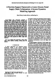
The Deben estuary is located on the coast of Suffolk in eastern England, UK (Fig. 1). The estuary extends south-eastwards for over 12 km from the town of Woodbridge to the sea just north of Felixstowe (Burningham and French, 2006). The Deben Estuary is an area of outstanding ecological importance resulting in International European and National designations - RAMSAR, SPA, SSSI and part of the Suffolk Area of Outstanding Natural Beauty ‐ (River Deben Association, 2014). The estuary is narrow and sheltered in its configuration and has a limited amount of fresh water inputs. The seabed in the offshore area contains a mixture of mud, fine sand and broken shell. The main characteristics of the bathymetry are the influence of the ridges of London Clay and sub-marine river channels, which are now buried and filled with fine sediments (HR Wallingford, 2002). The stretch of the Suffolk coast, where the Deben Estuary is located, is meso-tidal and mean spring tidal range varies from 3.2 m at Felixstowe Ferry to 3.6 m at Woodbridge (Hydrographic Office, 2000). The tidal length in the Deben estuary is approximately 18 km and the estuary has a mean spring tidal prism of around 17x106 m3. According to the National River Flow Archive – NRFA (2014) from measurements taken at Naunton Hall between 1964 and 2013 the peak spring tidal discharges through at the estuary inlet surpass 2000 m3/s. At 2 km upstream of the tidal limit, the mean flow of the River

1 2

College of Engineering, Swansea University, Singleton Park, Swansea, SA2 8PP, Wales, UK School of Engineering, Cardiff University, Queen's Buildings, The Parade, Cardiff, CF24 3AA, Wales, UK.

1

2

COASTAL ENGINEERING 2014

Deben is around 0.79 m3/s meaning that the estuary is well-mixed (NRFA, 2014). The inlet region has a landward flood tidal delta (Horse Sand) and a seaward ebb tidal delta (The Knoll). A single bar/spit extends from time to time from the Bawdsey foreland, (Fig. 1b inset). This stretch of coast is subject to the storm wave climate of the southern North Sea. The average wave heights is 0.96 m (offshore), with modal directions of 50% from the northeast and 32% southwest (Burningham and French, 2006). According to HR Wallingford (2002) waves from the Northeast are associated with the littoral drift pattern in the area. However, the orientation of the offshore sandbanks located near the estuary mouth is controlled by the strong tidal streams in the area. In the estuary inlet there is small wave propagation, and only fetch-limited wind waves are locally generated inside the estuary. a)

b)

Elevation (m OD) 10 9 8 7 6 5 4 3 2 1.8 1 0 -1 -2 -3 MLWS delineated in white

0

125

250

375

500 m

Figure 1. (a) Location and (b) bathymetric map of the Deben estuary.

The interaction of waves, tides and river flows are the main hydrodynamics drivers for tidal inlets (Boothroyd, 1985). Whereas the morphological aspects (morphology and behaviour of bedforms) depends on the nature and magnitude of sediment supply (FitzGerald et al., 2002). Land reclamation, of more than 2000 ha of intertidal mudflats and saltmarshes (approximately 25% of the tidal area), completed during the early 19 th century has considerably changed the Deben estuary (Beardall et al., 1991). Through this modification there is more than 25 km of defences in the estuary protecting 16 compartments from tidal inundation (more than 1400 ha) which once were estuary floodplains. According to the Suffolk estuarine strategies review (Posford Duvivier, 1999) many of the defences are in a deplorable state and realignment to restore tidal action in the compartment areas has been considered. Nevertheless, the stability of the shoreline downdrift of the area and the behaviour of the ebb-tidal delta may be modified due to the increase of the tidal prism. The Deben estuary is a RAMSAR site (wetland of international importance), Site of Special Scientific Interest, a Site of Special Protection (as defined by the EC Birds Directive). The main morphological aspects of the estuary are (Burningham and French, 2006):  Middle and upper reaches of the estuary: tidally dominated. o single meandering channel, (muddy intertidal flat and saltmarsh at the flanks) o entirely intertidal (upstream)  Landward of the estuary mouth, o Channel divides around a large shoal (Horse Sand), which is partly intertidal. o Main inlet channel between Bawdsey and Felixstowe Ferry is only 180m wide.  Course of the subtidal channel (offshore) defined by: o Position and extent of a historically mobile system of intertidal shoals known locally as The Knolls.  The inlet region of the Deben (Hayes, 1975) o A landward flood–tidal delta (Horse Sand), o A seaward ebb-tidal delta seaward (The Knolls). Bathymetry within and between the channels around the flood–tidal delta implies flood dominance to the northeast and ebb dominance to the southwest of Horse Sand.

3

COASTAL ENGINEERING 2014

The Deben estuary is known by being well documented in relation to bathymetric data and other surveys, as like Ordnance Surveys (OS) and Hydrographic charts. The Trinity House and the Harwich Haven Authority are responsible by doing, over the last decade, detailed surveys of the inlet and DebenFelixstowe frontage.

Figure 2. Historic bathymetric data sets for the Deben Estuary.

For this study thirteen bathymetric data sets were used (Fig. 2). This data covers mostly the inlet of the estuary and the adjacent coast. The data is supplied in form of gridded data (x, y, z). METHODOLOGY Inverse modelling

The approach adopted here is hybrid in nature, where simplified process dynamics are combined with a data-driven approach. Simplified process models have also been referred to as ‘behaviouroriented’ and ‘reduced physics’ models in the literature (e.g. Stive and De Vriend, 1995; Nicholas, 2010). To calculate the morphodynamic evolution, a form of equation governing this evolution is chosen on the basis of its ability to describe the observed changes, as opposed to being derived from first principles (Karunarathna et al., 2008). Such an approach has a well-established pedigree in the coastal engineering literature. Here a brief description of the method is given. The equation describing the time evolution of the bathymetry is thus taken as (Karunarathna et al., 2008; Reeve and Karunarathna, 2011): h ( x , y ,t )  2h  2h K x K y  S ( x , y ,t ) 2 t x y 2

(1)

where h(x,y,t) is bottom bathymetry of the area relative to a reference water level, Kx and Ky are the diffusion coefficients in the x and y coordinate directions, respectively, and S(x,y,t) is a source function that can be a function of both space and time. x and y are taken as cross-axis and long-axis directions. The diffusion process described by this equation will act to smooth sharp features of the bathymetry. The mmorphological changes are represented by diffusive and non-diffusive processes. The source term S(x,y,t) is added in order to represent the aggregate effect of all processes other than those described by diffusion (climate related drivers, human interference, etc.). Rescaling x and y to make coefficients of the spatial derivatives equal, Eq. 1 turns to: hˆ  2hˆ  2hˆ ˆ    S ( xˆ , yˆ ,t ) t xˆ 2 yˆ 2

(2)

4

COASTAL ENGINEERING 2014

where ^ indicates rescaled quantities. Dropping ^ for convenience, the governing equation may then be written as: h  2h  2h    S ( x , y ,t ) t x 2 y 2

(3)

or in operator (D) notation: ht  Dh  S

(4)

Then the source function is derived by inversion of Eq. 4: S ( x , y ,t m T / 2) 

 1  TD  TD  h (t m T )  exp h (t m ) exp   2   2  

T 

(5)

where T is time interval between two successive bathymetries h(t) and h(t +T). The diffusion coefficients are defined on the basis of values found in the literature (e.g., Baugh, 2004; Burgh and Manning, 2007) and then the source function for the period between two consecutive measurements is computed. The process is repeated in a pairwise fashion working through the sequence of historic bathymetry measurements h(x,y,t); generating a set of source functions. The source functions computed in this way have a well-defined structure, changing slowly relative to the measurement frequency. A detailed description of the numerical techniques necessary to determine the diffusion coefficients and to construct the source function is given in Spivack and Reeve (2000) and Karunarathna et al. (2008). Empirical Orthogonal Functions

A mathematical technique relying on what is termed Empirical Orthogonal Functions, (EOF), was used to analyse the source terms of the estuary obtained by the inverse method. The method separates the whole dataset into two sets of functions; one describing the spatial patterns of behaviour and the other the corresponding temporal variations. This information will be used to determine the patterns of behaviour of the source terms. The temporal functions can show trends or oscillations which can indicate likely patterns of behaviour in the future. By decomposing the set of source functions into their principal components, using Empirical Orthogonal Function (EOF) analysis, predictions of the source function for a particular period may be obtained by extrapolating the temporal coefficients of the EOFs. By this means a source function appropriate for forecasting can be constructed for use in the hybrid morphodynamic equations to obtain a forecast bathymetric morphology. The EOF technique was introduced into meteorological literature by Lorenz (1956) as a technique for analysing rainfall data. The analogous situation for coastal bathymetry is the analysis of beach levels along a fixed line. For example, the problem could be to determine the eigenfunctions of the variations in beach level in time along a fixed line. Also, the method has been used in the past to investigate variations in depth elevations and to find spatial/temporal patterns by applying the technique to sequences of bathymetric datasets. The EOF technique may be described briefly as follows. First, denote the discrete observations by g(l,tk), where 1 l L and 1 k K. The idea of EOF analysis is to express the data as: g (l ,t k ) 

L

 c p (t k ).e p (l )

(6)

p 1

where ep are the eigenfunctions of the square L x L correlation matrix of the data and cp are the coefficients describing the temporal variation of the pth eigenfunction. In practice, many fewer than L eigenfunctions may be required to capture a large proportion of the variation in the data. The correlation matrix, A, is calculated directly from the data. It has L x L elements which, if we denote these by amn with 1 m  L and 1 n  L, may be written as: a mn 

1 K .  g (m ,t k ).g ( n ,t k ) L.K k 1

(7)

5

COASTAL ENGINEERING 2014

The correlation matrix A is real and symmetric and has L real eigenvalues, p, with 1  p  L. The L corresponding eigenfunctions, ep(l), satisfy the matrix equation: Aep  p e p

(8)

The eigenfunctions of a real L x L symmetric matrix are mutually orthogonal. It is common practice to normalise the eigenvectors so they have unit length and thus: L

e p (l ).eq (l )   pq

(9)

l 1

where pq is the Kronecker delta. From Eq. 6 and Eq. 9, the coefficients cp may be calculated from: L

c p (t k )   g ( l ,t k ).e p ( l )

(10)

l 1

In the literature, and here, we refer to the above as the one-dimensional or ‘1-D’ EOF, as there is variability in one spatial dimension. For the two-dimensional EOF, the problem is to determine the eigenfunctions describing the variations in depth levels in time over an area in the (x,y)-plane. Denote the discrete measurements by h(xi ,yj ,tk), where 1  i  I, 1  j  J and 1  k  K. In contrast to the one-dimensional case there are several ways in which the data may be expanded in terms of eigenfunctions (e.g., Uda and Hashimoto, 1982; Hsu et al., 1994; Wijnberg and Terwindt, 1995). Here, we follow the procedure proposed by Reeve et al. (2001). Briefly, the two-dimensional grid of points is treated as one larger one-dimensional data set, and we use Eq. 5 with l covering all combinations of (xi,yj). Thus, we construct the correlation matrix, A, whose elements amn are the temporal correlation coefficients between seabed levels at any selected grid point (denoted by the m subscript) and those at every other point on the grid (denoted by the n subscript). The eigenfunction calculations then proceed as in the 1-D case. Each spatial eigenfunction can be plotted as a contour map by noting the correspondence between l and (xi,yj), and plotting the lth value of the eigenfunction at position (xi,yj). This procedure is more straightforward than other two-dimensional methods, makes no a priori assumption of separability of cross-shore and along-shore dependence, and the results are easier to interpret. Any similarity in behaviour at different points in the domain arises naturally from the analysis and will be evident in the results. Auto-regression method

After the EOF analysis was performed on the source terms data, the forecasts of the source terms were obtained using a fundamental auto-regression (AR) process. This process assumes that the value of the temporal eigenfunctions cp(tk), at a certain year tk, depends linearly on its r preceding values, c p t k   1c p t k 1  2c p t k 2   ..... r c p t k r    p (t k )

(11)

where r (model order) is the same for all L EOFs as defined in Eq. 6. There are different possibilities to calculate the constants β1,…., βr using auto-regression methods. Here we applied the method developed by Burg (1975), and the constants β1,…., βr are found through a Levinson–Durbin procedure involving the Yule–Walker equations (Marple, 1987): ,  1   1     r  2   r 1

1 1 

2 1 

 r 3  r  4  r 2  r 3

  r 2   r 1    1  1

 r 1    1    r  2   1 

 1     1             1    r 1   r 1  1    r    r 

(12)

where γ1,…., γr-1 are autocorrelation coefficients. The prediction error, εp(tk), is also minimize by this method. Pourahmadi (2001) pointed out that once a number r is chosen, then the corresponding β1,..., βr for each cp are uniquely defined. Burg’s algorithm has been widely used in Engineering. According to Percival and Walden (1993) this algorithm is mostly suitable for short time series and it always produces stationary autoregressive estimates. It is suitable for forecast based on EOF decomposition due to the similarity in the reproduction of stationary patterns as well. For the estimation of r, the procedure of Reeve et al. (2008) was followed.

6

COASTAL ENGINEERING 2014

In summary, the procedure used to calculate the forecasted source terms follows the flow chart shown in Fig. 3. Extrapolation AR Technique Temporal EOF Bathy Data

Inverse modelling

Source terms

Forecasted Temporal EOF

Reconstruction of source terms using EOF

EOF

Forecasted source terms Spatial EOF

Figure 3. Scheme showing the procedure to calculate the forecast of the source terms.

RESULTS Inverse modelling

Inverse solutions were obtained using the method described in the section above for each pair of consecutive bathymetric surveys to construct the source function corresponding to each survey interval. Fig. 4 show some selected source functions obtained from the inverse modelling. Several general features are apparent in the source function collectively, which complies with the assumptions used in the model. In general terms, there is no huge variation of source function from one interval to the other. Two significant features are persistent all the way through the results. One is related to the area of the left bank and the other refers to the spit of the inlet. Large scale features such as tidal channels, spit and sandbanks in the inlet estuary and the adjacent coast are noticeable in the source function.

Figure 4. Selected source functions obtained from the inverse modelling.

Large positive source functions changes in the tidal channel during the historic surveys period indicate consistent accretion in the left channel of the inlet and in some cases erosion in the middle channel (source term 1995-1996). This is in-line with the findings of Burningham and French (2006) where evidence of changes on the orientation was observed between surveys during the period between

7

COASTAL ENGINEERING 2014

1995 and 1997. Localised negative source functions in the north of the spit and the middle channel indicate erosion or sediment removal from those areas either by wave or tidal forcing. According to what is observed in the source functions and the corresponding bathymetric changes, there are notable differences between them. This is due to the large scale sediment diffusive process which plays a significant role in the long-term evolution of estuary morphology. It was found that there is no apparent difference to the structure of the source function when the diffusion coefficient is varied. One of the uses of predictions of future estuary morphological evolutions is that this can be of practical use for engineers and coastal planners. But for this, it is important to define the diffusion coefficients and the source function to predict the future behaviour of the estuary morphology. It is necessary to take into account that past historical behaviour provides a useful basis on which to extrapolate forward. That is to say that the forecast will not include changes that have not occurred in the past or in the data, that has been taken into consideration. The extrapolation of the source functions into the future may provide one means of predicting the morphological behaviour of the estuary. The key for a prediction is to investigate whether the sequence of source functions contains any spatial or more especially any particular temporal pattern that can be exploited. For this purpose, an Empirical Orthogonal Function (EOF) analysis was performed on the sequence of computed source functions. The method has been briefly described in the section above. Empirical Orthogonal Function (EOF) analysis

The EOF analysis was performed on the 12 source terms obtained from the inverse problem done over the 13 bathymetries. Table 1 summarises the results of this analysis for the first six eigenfunctions. It demonstrates that over 38.4% of the mean square of the data is contained in the first function and that 72.2% of the mean square of the data is captured by the first six. The mean square of the data is the average of the square of all the source functions values in the whole data set. The first eigenfunction corresponds to the mean source function over the period, with the subsequent eigenfunctions representing the variation about the mean. In this case, the 2nd through 6th eigenfunctions together account for over 72.2% of the variance about the mean. This is a large proportion of the variance for analyses of this kind and, as expected, the EOFs describe the variability in the source function very efficiently. Table 1. Eigenvalues and variance of the first six eigenfunctions. Eigenfunction 1 2 3 4 5 6

Normalised eigenvalue 0.38393 0.13567 0.10445 0.08047 0.06837 0.05610

Variance (%)

Cumulative Variance (%)

22.02 16.95 13.06 11.10 9.11

22.02 38.98 52.04 63.14 72.24

Fig. 5 show plots of 1st to 4th spatial eigenfunctions. The first eigenfunction gives the temporal mean value of the source function. The second eigenfunction, which depicts the shape of the strongest variation in the source function, shows a strong spatial structure with areas of maxima and minima. Most of these spatial patterns are a few hundreds of meters long and are elongated along the estuary. The 3rd eigenfunction shows spatial patterns which are of smaller scale to that of the 2 nd function. And that continues successively. The 5th and 6th eigenfunctions (not shown) have much less coherent spatial structure. The temporal variations of the source function are described by the temporal eigenfunctions. Fig. 6 shows first four temporal eigenfunctions. The first temporal eigenfunction is almost constant as expected because it corresponds to the temporal mean source function (not shown). In general, the temporal eigenfunctions show an oscillatory nature and an upward trend during the period concerned. The oscillations may be attributed to the bathymetry variations associated with large changes in the area of the spit and in the left side of the estuary mouth. Also it can be related to the historical changes in the channel lengths, ebb-jet angle, the throat cross sectional area and the bar depth of the Deben ebb-tidal delta (see Fig. 5, Burningham and French, 2006).

8

COASTAL ENGINEERING 2014

Figure 5. First 4 Spatial Orthogonal eigenfunctions.

Figure 6. The 2nd, 3rd and 4th temporal eigenvectors as functions of time. The first eigenvector is almost constant as it is resolving the mean value of the source functions.

Validation of extrapolation

After we obtained the temporal eigenfunctions following the analysis through EOF of the source functions from 1992-1993 to 1999-2000, we used an auto-regression (AR) technique that use the Burg’s algorithm for the extrapolation of the source terms (2000-2001, 2001-2002 and 2002-2003). Burg’s algorithm is particularly suitable for short time series. This makes it particularly suitable for forecasts based on EOF decompositions (Reeve et al. 2008). We followed the same technique described in Reeve et al. (2008). Fig. 7 shows the result of the validation of the extrapolation for the first four temporal eigenfunctions. According to the results, in the 1st and 3rd eigenfunctions there is an overprediction of the last value of the eigenfunctions, opposite to the 2nd temporal eigenfunction. In general, the results

9

COASTAL ENGINEERING 2014

show that the forecast of the source function captures the variability well in regions whose variation is more akin to standing wave behaviour, in agreement with the properties of the EOF technique. CEOF1 1

EOF amplitudes

0.8

CEOF2 0.6

Predicted Calculated

0.4

0.6

0.2

0.4

0

0.2

-0.2

0

-0.4

-0.2

-0.6

-0.4 1992

1994

1996

1998

2000

2002

2004

-0.8 1992

1994

1996

CEOF3

1998

2000

2002

2004

2000

2002

2004

CEOF4

0.5

1

EOF amplitudes

0.8 0.6 0.4 0 0.2 0 -0.2 -0.5 1992

1994

1996

1998

Years

2000

2002

2004

-0.4 1992

1994

1996

1998

Years

Figure 7. First 4 temporal eigenfunctions with their respective extrapolation of the source functions for the periods 2000-2001, 2001-2002 and 2002-2003.

Source function forecast

For the forecast of the source function, we followed the scheme in Fig. 3. Fig. 8 shows the calculated source function for the period between 2000 and 2001 and the predicted source function for the same period using the EOF method and the AR technique.

Figure 8. Source term calculated with the inverse technique (left panel) and Source term predicted with the EOF and AR techniques (right panel) for the period 2000 – 2001.

In general terms we can see from Fig. 8 that the forecasted source function looks very similar to the calculated with the inverse technique. The difference between the calculated source function for the

10

COASTAL ENGINEERING 2014

period 2000 – 2001 and the forecast of the source function coincide to a large degree with the regions of high variability in the estuary mouth. The left side of the shoreline (north part of the estuary mouth) is not well predicted by the forecast and the right side of this area are underpredicted. The channel is well predicted overall. And the bottom part of the area (the linear bank south of the estuary). This shows the technique performs relatively well for quasi-stationary features. CONCLUSIONS

A hybrid-reduced physics modelling approach has been applied to the Deben Estuary inlet for the period 1991 to 2003 for which we have annual bathymetry survey data. The work is on-going and we will present an analysis of the performance of the method for predicting the source terms of the estuary over the order of years as well as the robustness of the predictions. In this paper, the application of the model to predict mid-term morphodynamic evolution of estuaries is demonstrated and discussed. The present approach may be considered as an extended behaviour oriented approach for predicting morphodynamic evolution of estuaries. The model presented here is a hybrid between process-based and behaviour-oriented approaches. The technique used a governing equation that isolates diffusive and non-diffusive processes and describes long-term morphodynamic evolution, in our case, of an estuary tidal inlet. A source function is incorporated in order to take into account the effects of non-diffusive processes. This source function characterises the aggregation of all non-diffusive phenomena which lead to long-term morphodynamic evolution of an estuary. The success of the analysis depends on availability and precision of the historic bathymetric survey data. To obtain good quantitative results, an extensive historic data set covering a considerable time period is needed. The source functions were obtained from an inverse technique using historic bathymetric data of the Deben estuary, UK for a period of 13 years. According to this study, it was found that the source functions derived from the data are significantly different from the change in bathymetry during the corresponding time intervals. This means that the influence from diffusive processes to the morphodynamic evolution of the estuary is an important aspect. Furthermore, no rapid variation of the source function from one survey interval to the other was found. This gives an indication of a stable long-term morphodynamic evolution of the estuary against external (non-diffusive) forcing. Yearly scale changes of the Deben source terms are well predicted. Further analysis of source function is necessary for longer term predictions. An important spatial and temporal structure of the source function during the period covered by the historic survey data was found in the Empirical Orthogonal Function analysis. Extrapolating the sequence of mean source functions into the future will provide a means of estimating the source function when the governing equation is used in a predictive mode. Future work on the prediction of morphological changes will be done using the predicted source terms. ACKNOWLEDGMENTS

The authors acknowledge the support through the iCOASST project funded via the UK Natural Environment Research Council grant No. NE/J005606/1. The authors also wish to thank John French and Helene Burningham at University College London, UK for the provision of the Deben Estuary historic bathymetric data. REFERENCES

Baugh, J. 2004. Implementation of Manning Algorithm for Settling Velocity to an Estuarine Numerical Model, Technical Report No. TR 146, HR Wallingford Ltd, UK. Beardall, C.H., R.C. Dryden and T.J. Holzer. 1991. The Suffolk Estuaries. Segment Publications, Colchester. 77 pp. Boothroyd, J.C. 1985. Tidal inlets and tidal deltas. In: Davis Jr., R.A. (Ed.), Coastal Sedimentary Environments. Springer-Verlag, New York, pp. 445–532. Burg, J.P. 1975. Maximal Entropy Spectral Analysis. Ph.D. dissertation, Department of Geophysics, Stanford University, USA. Burgh, J., and A.J. Manning. 2007. An assessment of a new settling velocity parameterization for cohesive sediment transport modelling, Continental Shelf Research, 37 (13), 1835-1855.

COASTAL ENGINEERING 2014

11

Cowell P.J., P.S. Roy and R.A. Jones. 1992. Shoreface translation model: computer simulation of coastal-sand-body response to sea level rise, Mathematics and Computers in Simulation, 33, 603– 608. Burningham, H., and J. French. 2006. Morphodynamic behaviour of a mixed sand-gravel ebb-tidal delta: Deben Estuary, Suffolk, UK, Marine Geology, 225, 23–44. De Vriend, H., and J.S. Ribberink. 1996. Mathematical modelling of meso-tidal barrier island coasts, Part I: process based simulation models. In: Liu, P.L.F. (Ed.), Advances in Coastal and Ocean Engineering, 2, 151-197. FitzGerald, D.M., I.V. Buynevich, R.A. Davis Jr. and M.S. Fenster. 2002. New England tidal inlets with special reference to riverine-associated inlet systems, Geomorphology, 48, 179–208. Hanson H., S. Aarninkhof, M. Capobianco, J.A., Jiménez, M., Larson, R.J., Nicholls, N.G. Plant, H.N. Southgate, H.J. Steetzel, M.J.F. Stive, and H.J. De Vriend. 2003. Modelling of coastal evolution on yearly to decadal time scales, Journal of Coastal Research, 19(4), 790–811. Hayes, M.O. 1975. Morphology of sand accumulation in estuaries: an introduction to the symposium. In: Cronin, L.E. (Ed.), Estuarine Research. Academic Press, New York, pp. 3– 22. HR Wallingford. 2002. Southern North Sea Sediment Transport Study (phase 2). HR Wallingford Report, EX, p. 4526. Hsu, T-W., S-H. Ou, and S-K. Wang. 1994. On the prediction of beach changes by a new 2-D empirical eigenfunction model, Coastal Engineering, 23, 255-270. Hydrographic Office. 2000. Admiralty tide tables: United Kingdom and Ireland (including European channel ports). Hydrographer of the Navy. 440 pp. Karunarathna, H., D.E. Reeve, and M. Spivack. 2008. Long term morphodynamic evolution of estuaries: an inverse problem, Estuarine Coastal and Shelf Science, 77, 386–395. Kragtwijk N.G., T.J. Zitman, M.J.F. Stive, Z.B. Wang. 2004. Morphological response of tidal basins to human intervention, Coastal Engineering, 51, 207–221. Lorenz, E.N. 1956. Empirical orthogonal functions and statistical weather prediction. Report 1. Dept. of Meteorology, Massachusetts Institute of Technology,Cambridge, USA, 49 pp. Marple, S.L.Jr. 1987. Digital spectral analysis with applications. Prentice Hall, Englewood Cliffs, New Jersey, USA. Nicholas, A.P. 2010. Reduced complexity modeling of free bar morphodynamics in alluvial channels, Journal of Geophysical Research, 115, F04021, doi:10.1029/2010JF001774. NRFA, 2014. National River Flow Archive. http://www.nwl.ac.uk/ih/nrfa/. Posford Duvivier. 1999. Suffolk estuarine strategies: river Deben. Strategy Report: Volume 1 Main Report. Environment Agency: Anglian Region, CP505(163). 61 pp (plus appendices). Percival, D.B., and A.T. Walden. 1993. Spectral Analysis for Physical Applications: Multitaper and Conventional Univariate Techniques. CUP, Cambridge, UK. Pourahmadi, M. 2001. Foundations of time series analysis and prediction theory. Wiley, New York, 448 pp. Reeve, D.E., B. Li, and N. Thurston. 2001. Eigenfunction analysis of decadal fluctuations in sandbank morphology, Journal of Coastal Research, 17(2), 371-382. Reeve D.E., J.M. Horrillo-Caraballo and V. Magar. 2008. Statistical analysis and forecasts of long-term Sandbank Evolution at Great Yarmouth, UK. Estuarine, Coastal and Shelf Science, doi: 10.1016/j. ecss.2008.04.016. Reeve, D.E. and H. Karunarathna. 2011. A statistical–dynamical method for predicting estuary morphology, Ocean Dynamics, 61, 1033–1044. River Deben Association. 2014. Deben Estuary Partnership. http://www.riverdeben.org/category/debenestuary-partnership/, [accessed 29 July 2014], 2014. Spivack, M. and D.E. Reeve. 2000. Source reconstruction in a coastal evolution equation. Journal of Computational Physics, 161, 169–181. Stive, M.J.F. and H.J., De Vriend. 1995. Modelling shore-face profile evolution, Marine Geology, 126, 235–248. Uda, T. and H. Hashimoto. 1982. Description of beach changes using an empirical predictive model of beach profile changes, Proceedings of 18th International Conference on Coastal Engineering, ASCE, 1405-1418. Wijnberg, K.M. and J.H.J. Terwindt. 1995. Extracting decadal morphological behaviour from highresolution, long-term bathymetric surveys along the Holland coast using eigenfunction analysis, Marine Geology, 126, 301-330.