1 An Observational Study of the Relationship between ... - CiteSeerX

An Observational Study of the Relationship between Cloud, Aerosol and Meteorology in Broken Low-Level Cloud Conditions Norman G. Loeb1 and Gregory L. Schuster NASA Langley Research Center, Hampton, Virginia1

Journal of Geophysical Research- Atmospheres Revised March 2008

1

Corresponding Author Address: Dr. Norman G. Loeb, Mail Stop 420, NASA Langley

Research Center, Hampton, VA 23681-2199, U.S.A. (757) 864-5688 (office); (757) 8647996 (fax); Email: norman.g.loeb@ nasa.gov

1

1

Abstract

2

Global satellite analyses showing strong correlations between aerosol optical depth and

3

cloud cover have stirred much debate recently. While it is tempting to interpret the results

4

as evidence of aerosol enhancement of cloud cover, other factors such as the influence of

5

meteorology on both the aerosol and cloud distributions can also play a role, as both

6

aerosols and clouds depend upon local meteorology. This study uses satellite

7

observations to examine aerosol-cloud relationships for broken low-level cloud regions

8

off the coast of Africa. The analysis approach minimizes the influence of large-scale

9

meteorology by restricting the spatial and temporal domains in which the aerosol and

10

cloud properties are compared. While distributions of several meteorological variables

11

within 5°×5° latitude-longitude regions are nearly identical under low and high aerosol

12

optical depth, the corresponding distributions of single-layer low cloud properties and

13

top-of-atmosphere radiative fluxes differ markedly, consistent with earlier studies

14

showing increased cloud cover with aerosol optical depth. Furthermore, fine-mode

15

fraction and Angstrom Exponent are also larger in conditions of higher aerosol optical

16

depth, even though no evidence of systematic latitudinal or longitudinal gradients

17

between the low and high aerosol optical depth populations are observed. When the

18

analysis is repeated for all 5°×5° latitude-longitude regions over the global oceans (after

19

removing cases in which significant meteorological differences are found between the

20

low and high aerosol populations), results are qualitatively similar to those off the coast

21

of Africa.

22 23

2

1

1. Introduction

2

Many questions surround the use of passive satellite observations for studying

3

aerosol-cloud interactions. Several studies (e.g., Coakley et al. 1987; Han et al, 1994;

4

Bréon et al., 2002; Sekiguchi et al., 2003) have used a range of techniques to observe the

5

first indirect effect (Twomey, 1977), while others have found evidence of precipitation

6

suppression (the second indirect effect, Albrecht, 1989) in regions of biomass burning

7

smoke (Rosenfeld 1999; Andreae et al. 2004; Koren et al. 2004), urban and industrial air

8

pollution (Rosenfeld 2000, Matsui et al., 2004), and desert dust (Rosenfeld et al. 2001).

9

More recently, satellite analyses have revealed a persistent correlation between cloud

10

fraction (f) and aerosol optical depth (τa) in regions influenced by marine aerosol, smoke,

11

dust and industrial air pollution (Ignatov et al., 2005; Loeb and Manalo-Smith 2005;

12

Kaufman et al., 2005; Matheson et al., 2006).

13

While results from studies showing a correlation between f and τa are qualitatively

14

similar, their interpretation varies greatly. Ignatov et al. (2005) note that the aerosol-cloud

15

correlations are either “real” (increased hygroscopic aerosol particles that influence cloud

16

formation) or artifacts of the retrievals (residual cloud in the imager field-of-view). Loeb

17

and Manalo-Smith (2005) point to the importance of meteorology: f and τa are both

18

correlated with relative humidity (RH) and wind speed. As RH increases, water uptake by

19

aerosols (determined by the solubility of the particle mass) changes the aerosol particle

20

size, density, refractive index, and scattering extinction (e.g., Clarke et al. 2002). This,

21

together with larger wind speeds (which increase sea salt particles), lead to larger τa.

22

Mauger and Norris (2007) used data from the North Atlantic to argue that the history of

23

meteorological forcing controls both AOD and cloud fraction. In their analysis, scenes 3

1

with large AOD and large cloud fraction had origins closer to Europe and experienced

2

greater lower tropospheric static stability 2–3 days prior to the satellite observation than

3

did scenes with small AOD and small cloud fraction. Matheson et al. (2006) raise

4

additional possible reasons for the aerosol-cloud correlations, including increased particle

5

production near clouds, an increase in aerosol size caused by in-cloud processing, and

6

sunlight reflected by nearby clouds enhancing the illumination of the adjacent cloud-free

7

pixels causing τa to be overestimated. In contrast, Kaufman et al. (2005) conclude that

8

most of the correlation is explained by the aerosol indirect effect, and that there is a low

9

probability the results are due to errors in the data or coincidental, unresolved, changes in

10

meteorological conditions that also lead to higher τa.

11

A possible physical mechanism by which the aerosols interact with clouds to

12

produce an increase in f is through precipitation suppression, or the second indirect effect.

13

An increase in aerosol abundance causes an increase in the number of cloud-condensation

14

nuclei (CCN), leading to smaller cloud droplets, reduced precipitation, longer cloud

15

lifetimes, and increased f. Implicit in the argument that the satellite-derived aerosol-cloud

16

correlation is evidence of the aerosol indirect effect is the assumption that satellite-

17

derived τa is correlated with CCN concentration. However, most CCN are too small to

18

contribute to radiances observed by satellite instruments. While no definitive proof of a

19

relationship between column optical depth and CCN exists, a study by Kapustin et al.

20

(2006) suggests that under certain conditions there is a strong link. Kapustin et al. (2006)

21

derive a proxy for CCN (from size distribution measurements), which they relate to

22

aerosol optical properties, such as the aerosol index (AI, product of τa and Angstrom

23

exponent, α), a parameter often used by the satellite community because it is more

4

1

sensitive to the accumulation mode aerosol concentration (e.g., Deuze et al., 2001;

2

Nakajima et al., 2001). Kapustin et al. (2006) conclude that correlations between optical

3

parameters and the CCN proxy appear to work best in conditions of pollution aerosol

4

with moderate amounts of coarse dust, and that the correlation between aerosol index and

5

CCN is likely strongly dependent upon RH.

6

In this study, satellite observations are used to examine aerosol-cloud

7

relationships for broken low-level cloud regions off the coast of Africa. The analysis

8

seeks to minimize the influence of large-scale meteorology by restricting the spatial and

9

temporal domains in which the aerosol and cloud properties are compared. Each day,

10

cloud properties and various large-scale meteorological variables are sorted by aerosol

11

optical depth and the resulting distributions are directly compared.

12

2. Observations and Methodology

13

To investigate relationships between aerosols, clouds and meteorology, a global

14

dataset with 1° spatial and daily temporal resolution is created which combines several

15

data sources. We combine radiative fluxes from the Clouds and the Earth’s Radiant

16

Energy System (CERES) (Wielicki et al., 1996), cloud and aerosol properties from the

17

MODerate resolution Imaging Spectroradiometer (MODIS), meteorological parameters

18

from the Global Modeling and Assimilation Office (GMAO)'s Goddard Earth Observing

19

System DAS (GEOS-DAS V4.0.3) product (Suarez et al., 2005), wind speed divergence

20

derived from the SeaWinds instrument on the QuikSCAT satellite, and aerosol type

21

information from the Model for Atmospheric Transport and Chemistry (MATCH)

22

(Collins et al., 2001). CERES fluxes, MODIS aerosol and cloud properties, and GEOS-4

23

parameters are from the Terra Edition2B_rev1 Single Scanner Footprint TOA/Surface 5

1

Fluxes and Clouds (SSF) product (Loeb et al., 2003, 2005). The SSF consists of cloud

2

property retrievals from Minnis et al. (1998) and Minnis et al. (2003), and aerosol

3

property retrievals from the MOD04 product (Remer et al. 2005), and a second aerosol

4

retrieval algorithm applied to MODIS (Ignatov and Stowe 2002). In this study, we use

5

collection 4 MODIS products.

6

We consider one month (September 2003) of data off the coast of Africa between

7

0°S-30°S and 50°W-10°E and restrict the analysis to regions dominated by sulfate

8

aerosol according to the MATCH model. Only single-layer low clouds in 1° regions with

9

both cloud and aerosol retrievals are considered. Each day, cloud and aerosol retrievals in

10

every 5°×5° region are sorted into two populations: (I) 1° subregions with MODIS τa less

11

than or equal to the mean 5°×5° value (); and (II) 1° subregions with τa greater than

12

. Stratifying each 5°×5° region each day into two groups ensures that both groups are

13

influenced by the same large-scale meteorological influences. Next, distributions of

14

meteorological, cloud, aerosol and radiative flux parameters from the two populations are

15

directly compared. To define the above two populations MODIS 0.55-µm τa retrievals

16

are used (Remer et al., 2005). In the analysis we only consider low-level cloud properties

17

from 1° sub-regions in which the high cloud coverage is < 2.5%, and a valid MODIS

18

AOD is observed within the region. A minimum of two 1° sub-regions satisfying these

19

criteria are required in order for a 5° region to be included in the analysis. This typically

20

results in 2 to 10 1° sub-regions per 5° region.

6

1 2

3. Results Figs. 1a-f show relative frequency distributions of 750-1000 mb potential

3

temperature difference (θ -θ

4

(SST), 10-m wind speed (w ), QuikSCAT-based wind divergence (∇w), and wind

5

direction (wd). Although not a comprehensive list, these meteorological parameters are

6

correlated with the occurrence of low-level cloud amount (e.g., Klein, 1997; Xu et al.,

7

2005). As shown, nearly identical distributions are obtained for each of these parameters,

8

confirming that the two aerosol populations are influenced by the same large-scale

9

meteorological influences. As indicated in Table 1, which shows the sample mean values,

10

differences between the means of the distributions are not significant at the 95%

11

confidence level.

750

), precipitable water (p ), sea-surface temperature

1000

w

s

12

The corresponding aerosol property distributions are shown in Figs. 2a-c. By

13

definition, τa values for population II are larger than those for population I (Fig. 2a). The

14

overall mean τa for population I is 0.11 compared to 0.15 for population II (Table 1).

15

Interestingly, population II seems to have a larger mass fraction of smaller aerosol

16

particles than population I, as shown in both the fine-mode fraction (η) (Fig. 2b) and

17

Angstrom exponent (α) (Fig. 2c) distributions. η is obtained directly from the MOD04

18

aerosol product while α is computed using MODIS aerosol optical depth retrievals at

19

0.55-µm and 0.86-µm. The mean η (α) ranges from 0.37 (0.42) for population I to 0.43

20

(0.62) for population II. Sample mean differences between the populations are significant

21

at the 95% level for both parameters (Table 1). In fact, the difference between the means

22

exceeds the 95% confidence interval (σ95) by a factor of 2 to 3. Kaufman et al. (2005)

23

also found an increase in η in the transition from clear oceanic air to high dust or smoke 7

1

concentrations. However, in contrast to the Kaufman et al. (2005) results, the aerosol

2

populations considered in Fig. 2 are restricted spatially (i.e., to 5°×5° regions) and

3

experience similar large-scale meteorology. To ensure that spatial gradients within the

4

individual 5°×5° regions aren’t contributing to the differences in η and α between the

5

two populations, Figs. 2d shows histograms of the difference between the mean latitudes

6

for the 1° subregions used to define the two populations, and Fig. 2e shows the difference

7

between the corresponding mean longitudes. In each case, the peak in the distributions of

8

mean latitude and longitude difference is close to zero, indicating that local gradients in

9

aerosol optical depth aren’t responsible for the differences in η and α.

10

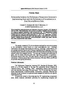
Figs. 3a-f and Table 1 compare TOA flux and cloud property distributions

11

between populations I and II. SW TOA flux, f, surface-cloud top temperature difference

12

and cloud liquid water path all tend to be significantly larger in population II compared to

13

population I. The CERES LW TOA flux is smaller for population II, consistent with the

14

larger surface-cloud top temperature difference, cloud fraction and liquid water path.

15

Similar results are obtained when we restrict the analysis to regions dominated by smoke

16

aerosol (as opposed to sulfate) according to the MATCH model.

17

The one cloud parameter that shows no significant difference between the two

18

populations is droplet effective radius (re). To investigate this further, Fig. 4a-d shows

19

differences between population II and population I cloud properties as a function of the

20

corresponding difference in 0.55 µm aerosol optical depth (black circles). In order to

21

reduce sampling noise, the averages were computed in discrete intervals of Δτa of width

22

0.02. The histogram in each plot indicates the number of 5º regions falling in each

23

interval. For Δτa < 0.08, corresponding to approximately 90% of the regions, Δre is 8

1

slightly positive with an average value of 0.23 µm. It is only in the top 10% of the

2

distribution (i.e., Δτa > 0.08) that we see the expected anticorrelation between Δre and

3

Δτa. For Δτa > 0.08, Δre has a mean of -0.54 µm, and reaches -2 µm at Δτa=0.15. Since

4

most of the samples have small Δτa, the overall mean re difference between populations I

5

and II is small. In contrast, the other cloud parameters (Fig.s. 4b, c and d) all tend to show

6

positive differences at all intervals of Δτa. In addition Δf and Δτc show a positive

7

correlation with Δτa.

8

To examine relationships between aerosol and cloud properties in other locations,

9

the analysis is extended to all 5°×5° oceanic regions in which MOD04 aerosol retrievals

10

are available. In order to acquire sufficient sampling, all September days from 2002

11

through 2005 are considered. In addition, to minimize the influence of large-scale

12

meteorology, only 5°x5° regions in which the difference in each of the meteorological

13

parameters (i.e., p , w , wd, ∇w, θ -θ

14

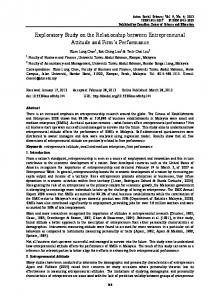
is less than the 95% confidence interval are included. Figs. 5a-b show the resulting

15

differences in cloud fraction (Fig. 5a) and fine-mode-fraction (Fig. 5b) between

16

populations I and II. Differences are calculated from the product ΔX/Δτa × , where

17

ΔX is the mean difference in X between populations I and II, and is the overall 5°x5°

18

mean τa. In the majority of regions, populations with larger τa also have larger f and η ,

19

consistent with results in Figs. 2 and 3. Fig. 5 clearly suggests these correlations are quite

20

robust and occur in most oceanic regions. At higher latitudes the number of 5°x5° regions

21

satisfying our selection criteria decreases dramatically, especially over the Southern

22

Ocean between 40°S-60°S where cloud cover is generally quite large. Regions with

23

negative δη (e.g., off the coast of California, in the Gulf of Mexico, over the

w

s

750

1000

, SST, and SST-T ) between the two populations c

9

1

Mediterranean and Black Seas, and at high latitudes) are likely spurious as these regions

2

were generally sampled fewer than 5 days during the entire period considered.

3

4. Discussion

4

While it is tempting to conclude that correlations between aerosol and cloud

5

properties are due to indirect effects of aerosols, other explanations should also be

6

considered. The results presented here suggest that large-scale meteorology is likely not a

7

factor since identical distributions of several meteorological variables were obtained for

8

both aerosol populations. An alternate interpretation of the results in Section 3 is that

9

cloud contamination in the τa retrievals is responsible for the apparent aerosol-cloud

10

correlations. For example, in regions of higher f within a 5°×5° region, cloud

11

contamination may lead to higher τa, causing population II to be cloudier. However, Fig.

12

2b and 2c show that the fine-mode fraction and Angstrom exponent are actually larger for

13

population II, which does not support this hypothesis. If cloud contamination were the

14

dominant reason for differences between populations I and II, one would expect popu-

15

lation II to have less fine-mode aerosols, not more.

16

A critical parameter missing in this analysis is RH. Klein (1997) used 25-years of

17

radiosonde data from ocean weather station November, located halfway between San

18

Francisco and Hawaii, to investigate correlations between low cloud amount and several

19

meteorological variables. He found that low cloud amount is positively correlated with

20

RH in the cloud layer (~850–950 mb), and negatively correlated with RH immediately

21

above the trade inversion. Similar conclusions were reached in Slingo (1980), Albrecht

22

(1981), and Bretherton et al. (1995). At the same time, τa also increases with RH (Clarke

23

et al., 2002). Thus, one could reasonably argue that the aerosol-cloud correlations 10

1

observed in the satellite observations are nothing more than the response of both the

2

clouds and aerosols to changes in RH. Unfortunately, RH data from meteorological data

3

assimilation

4

(parameterizations) in the models.

models

are

unreliable

due

to

poor

boundary

layer

physics

5

To investigate theoretically if increasing RH can produce increases in Angstrom

6

exponent similar to those in this study, we examine the effect of aerosol swelling on α

7

and the effective radius (Hansen and Travis, 1974) for an aerosol size distribution

8

representative of marine environments. We begin with a dry bimodal aerosol size

9

distribution that is composed of ammonium sulfate in mode 1 and sea salt in mode 2:

10 11 12

(1) where Ci represents the modal volume concentration (accumulation or coarse), Ri is the

13

median or geometric mean modal radius, and σi is the variance or width of each mode.

14

The accumulation mode of our assumed size distribution has dry values of R1=0.106 µm

15

and σ1=0.4; the coarse mode has dry values of R2=1.42 µm and σ2=0.78. These size

16

distribution parameters are based upon the AERONET climatology at Ascension Island

17

(Smirnov et al., 2002), located in the Southern Atlantic Ocean near the middle of our

18

study area (i.e., 14.415° West, 7.976° South). The radii quoted here are slightly smaller

19

than Smirnov et al. (2002) because the AERONET climatology represents wet aerosols.

20

We arrived at our dry radii by assuming that the accumulation mode is composed of

21

hydrated ammonium sulfate and that the coarse mode is composed of hydrated sea salt at

22

a relative humidity of 70%.

11

1

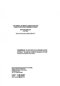
We model the hygroscopic growth of these two modes using nine different

2

accumulation mode fractions, as shown in Figure 6. We computed the Angstrom

3

exponents using Mie theory (Wiscombe, 1980) and derived the wet aerosol refractive

4

indices from a subroutine available at http://gacp.giss.nasa.gov/data_sets/ (courtesy of

5

Andy Lacis). This subroutine uses the spectral refractive indices of dry ammonium

6

sulfate (Toon et al., 1976) dry sea salt (Shettle and Fenn, 1979), and water (Hale and

7

Querry, 1973) to compute the spectral refractive index of aqueous mixtures using the

8

water activities and refractive indices at the 0.6328 µm wavelength (Tang and

9

Munkelwitz, 1991,1994; Tang, 1996).

10

We first consider the hygroscopic growth of the accumulation mode of this size

11

distribution, which is shown in the upper left corner of Figure 6 (i.e., C1/(C1+C2)=1 ). In

12

this case, the Angstrom exponent has a value of α=3 when RH=55%, and decreases to a

13

value of α=1.7 when relative humidity increases to RH=99%. Hence, the Angstrom

14

exponent decreases as the aerosol effective radius increases, which is consistent with

15

conventional expectations (Angstrom, 1929; Schuster et al., 2006). Coarse mode growth

16

does not have the same impact on the Angstrom exponent, however (i.e., C1/(C1+C2)=0

17

in Figure 6). This is because the Mie extinction efficiency for the large coarse particles

18

does not exhibit dramatic changes over the coarse particle size range. Finally, Figure 6

19

indicates that bimodal mixtures of these two modes can result in Angstrom exponents

20

that can either increase or decrease as aerosols swell, depending upon the initial

21

accumulation mode fraction and relative humidity. In general, dry accumulation mode

22

fractions of less than 0.6 tend to produce an increase in the Angstrom exponent as

23

aerosols swell, while dry accumulation mode fractions greater than 0.8 tend to produce a 12

1

decrease in the Angstrom exponent as aerosols swell (for these lognormal parameters).

2

We also note that bimodal distributions with a hygroscopic fine mode and a hydrophobic

3

coarse mode (such as dust) can also produce increases in the Angstrom exponent as the

4

fine mode swells (not shown).

5

We can use these theoretical aerosol growth curves to understand how swelling

6

might be responsible for the change in α that we observed in our South Atlantic study.

7

Recall that the mean α ranges from 0.42 for population I to 0.62 for population II, which

8

is indicated by the dashed lines in Figure 6. Hence, aerosol swelling can produce the

9

observed δα between populations I and II if the dry accumulation mode fraction is about

10

0.3 and the average relative humidity varies from 55 to 96% between the two regions.

11

The same δα could also be achieved with our assumed size distributions over a much

12

smaller difference in humidity (97-99%) if the dry accumulation mode fraction is only

13

0.2 (of course, intermediate ranges of relative humidity are also possible with

14

intermediate accumulation mode fractions). We also note that the wet accumulation mode

15

fractions vary from 0.05 to 0.12 for this range of α and these size distributions (not

16

shown), which is consistent with observations in that region (Quinn et al., 2001; Smirnov

17

et al., 2002).

18

Another possible explanation for the strong aerosol-cloud correlations in the

19

satellite data is the so-called “cloud adjacency effect”, whereby cloud free pixels are

20

brightened (or shadowed) by reflected light from surrounding clouds (Kobayashi et al.,

21

2000; Cahalan et al., 2001; Wen et al., 2001, 2006, 2007; Nikolaeva et al., 2005). Wen et

22

al. (2006) used Monte Carlo simulations of TOA reflectance to show that the overall

23

effect of clouds is to enhance the reflectance in clear regions leading to systematically 13

1

higher aerosol optical depth estimates for pixels closer to clouds. Furthermore, Wen et al.

2

(2007) and Marshak et al. (2007) showed that the enhancement is more pronounced at

3

shorter wavelengths leading to an apparent bluing of aerosols near clouds. Marshak et al.

4

(2007) argue that the enhancement in the cloud-free column radiance comes from the

5

enhanced Rayleigh scattering due to the presence of surrounding clouds. This

6

interpretation would cause an apparent increase in η and α with cloud fraction, consistent

7

with the results in Section 3.

8

If Rayleigh scattering above the cloud layer is indeed responsible for the bluing of

9

the aerosols at TOA, this may explain why the same effect is not observed at the surface

10

by Koren et al. (2007). Using Aerosol Robotic global network (AERONET) data in the

11

vicinity of clouds, they found that τa increased and α decreased with decreasing distance

12

from a cloud, suggesting that aerosol particles become larger near clouds. Koren et al.

13

(2007) also examined variations in MODIS spectral reflectances as a function of distance

14

from a cloud. They found larger relative increases in reflectance with decreasing distance

15

from a cloud at 2.1 µm than at 0.47 µm. We note that such relative changes in spectral

16

reflectance don’t necessarily mean that Angstrom exponent and/or fine-mode fraction

17

changed. As a test, we performed radiative transfer calculations using the coupled Ocean

18

Atmosphere Radiative Transfer (COART) model (Jin et al., 2006) with maritime aerosols

19

from Hess et al. (2005) at 0.55 µm aerosol optical depths of 0.05 and 0.15. We found that

20

the relative reflectance difference at these two optical depths was five times larger at 2.1

21

µm than at 0.47 µm with no change in aerosol size distribution. Cleary, a more

22

meaningful comparison would be to examine variations in τa as a function of distance

23

from the cloud at different wavelengths rather than relative reflectance. 14

1

5. Summary

2

Satellite observations are used to examine aerosol-cloud relationships using a

3

sampling strategy that minimizes the influence of large-scale meteorology on the aerosol-

4

cloud property comparisons. One month of CERES and MODIS aerosol, cloud and

5

radiation data from September 2003 off the coast of Africa are considered. Each day,

6

cloud and aerosol properties within individual 5°x5° regions are sorted into two

7

populations according to whether aerosol optical depth retrievals in 1°x1° subregions are

8

less than or greater than the 5°x5° regional mean aerosol optical depth. Distributions of

9

meteorological, cloud, aerosol and radiative flux parameters are then compared for the

10

two populations for all 5°x5° regions during the entire month.

11

While distributions of several meteorological parameters (e.g., precipitable water,

12

wind speed and direction, wind divergence, 750-1000 mb potential temperature

13

difference, SST) showed no significant differences between the low and high aerosol

14

optical depth populations, the cloud properties and TOA radiative fluxes showed marked

15

differences. The population with larger aerosol optical depth had systematically higher

16

cloud cover, liquid water path, and SW TOA flux. Temperature differences between sea-

17

surface temperature and cloud-top also were greater and the LW TOA flux was smaller,

18

suggesting higher cloud tops. In addition, fine-mode fraction and Angstrom exponent

19

were significantly larger for the high aerosol optical depth population, even though no

20

evidence of systematic latitude or longitude gradients between the aerosol populations

21

was observed. Repeating the analysis for all 5°×5° latitude-longitude regions over the

22

global oceansafter removing cases in which significant meteorological differences

23

were foundyielded similar results too those obtained off the African coast. 15

1

The lack of a meteorological explanation for the strong correlations should not be

2

interpreted as evidence of aerosol enhancement of cloud cover. Other possible

3

explanations include artifacts of the aerosol retrievals near clouds, aerosol swelling, in-

4

cloud processing, and particle production near clouds. Further research is needed to

5

improve our understanding of these processes.

Acknowledgements

6 7

This research has been supported by NASA Interdisciplinary Research in Earth

8

Science, Aerosol Impacts on Clouds, Precipitation, and the Hydrologic Cycle and by the

9

NASA CERES project. The CERES SSF data were obtained from the Atmospheric

10

Sciences Data Center at the NASA Langley Research Center. We are grateful for access

11

to the subroutines made available by Dr. Andy Lacis at the Global Aerosol Climatology

12

Project (GACP) webpage. We thank Drs. James A. Coakley, Jr., Bruce A. Wielicki,

13

Kuan-Man Xu, Lorraine Remer, Alexander Marshak, Wenying Su and Wenbo Sun for

14

stimulating discussions.

16

6. References Albrecht, B.A., 1989: Aerosols, cloud microphysics, and fractional cloudiness, Science, 245, 1227-1230. Albrecht, B. A., 1981: Parameterization of trade-cumulus cloud amount. J. Atmos. Sci., 38, 97–105. Andreae, M. O., D. Rosenfeld, P. Artaxo, A. A. Costa, G. P. Frank, K. M. Longo, and M. A. F. Silva-Dias, 2004: Smoking Rain Clouds over the Amazon. Science, 303, 1337-1342. Angstrom, A. (1929), On the atmospheric transmission of sun radiation and on dust in the air, Geografiska Annaler, 11, 156–166. Bréon, F.-M., D. Tanré, and S. Generoso, 2002: Aerosol effect on cloud droplet size monitored from satellite. Science, 295, 834–838. Bretherton, C.S., E. Klinker, A. K. Betts, and J. Coakley, 1995: Comparison of ceilometer, satellite, and synoptic measurements of boundary layer cloudiness and the ECMWF diagnostic cloud parameterization scheme during ASTEX. J. Atmos. Sci., 52, 2736–2751. Cahalan, R. F., L. Oreopoulos, G. Wen, A. Marshak, S.-C. Tsay, and T. DeFelice, 2001: Cloud Characterization and Clear Sky Correction from Landsat 7. Remote Sens. Environ., 78, 83-98. Clarke, A. D., and Coauthors, 2002: INDOEX aerosol: A comparison and summary of chemical, microphysical, and optical properties observed from land, ship, and aircraft. J. Geophys. Res., 107, 8033, doi:10.1029/2001JD000572. Coakley, J.A., Jr., R. L. Bernstein, P. A. Durkee, 1987: Effect of ship-stack effluents on cloud reflectivity, Science, 237, 1020-1022. Collins, W.D., P.J. Rasch, B.E. Eaton, B.V. Khattatov, J.-F. Lamarque, and C.S. Zender, 2001: Simulating aerosols using a chemical transport model with assimilation of satellite aerosol retrievals: Methodology for INDOEX. J. Geophys. Res., 106, 7313–7336. Deuze, J. L., et al., 2001: Remote sensing of aerosols over land surfaces from POLDERADEOS-1 polarized measurements, J. Geophys. Res., 106, 4913– 4926. Hale, G. M., and M. R. Querry (1973), Optical constants of water in the 200-nm to 200micrometer wavelength region, Appl. Opt., 12(3), 555. Han, Q., W. B. Rossow, and A. A. Lacis, 1994: Near-global survey of effective droplet radii in liquid water clouds using ISCCP data. J. Clim., 7, 465-497. Hansen, J., and L. Travis (1974), Light scattering in planetary atmospheres, Space Sci. Rev., 16, 527–610.

17

Hess, M., P. Koepke, and I. Schult, 1998: Optical properties of aerosols and clouds: The software package OPAC. Bull. Amer. Meteor. Soc., 79, 831-844. Ignatov, A., and Coauthors, 2005: Two MODIS aerosol products over ocean on the Terra and Aqua CERES SSF datasets. J. Atmos. Sci., 62, 1008–1031. Jin, Z., T.P. Charlock, K. Rutledge, K. Stamnes, and Y. Wang, 2006: Analytical solution of radiative transfer in the coupled atmosphere-ocean system with a rough surface. Appl. Opt., 45, 7443-7455. Kapustin, V.N., A. D. Clarke, Y. Shinozuka, S. Howell, V. Brekhovskikh, T. Nakajima, and A. Higurashi, 2006: On the determination of a cloud condensation nuclei from satellite: Challenges and possibilities, J. Geophys. Res., 111, D04202, doi:10.1029/2004JD005527. Kaufman, Y. J., I. Koren, L. A. Remer, D. Rosenfeld, and Y. Rudich, 2005: The effect of smoke, dust, and pollution aerosol on shallow cloud development over the Atlantic Ocean, Proc. Natl. Acad. Sci. U.S.A., 102(32), 11,207– 11,212.¶ Klein, S.A., 1997: Synoptic variability of low-cloud properties and meteorological parameters in the subtropical trade wind boundary layer, J. Climate, 10, 2018-2039. Kobayashi T., K. Masuda, M. Sasaki, J. Mueller, 2000: Monte Carlo simulations of enhanced visible radiance in clear-air satellite fields of view near clouds. J. Geophys. Res., 105, 26569-26576. Koren, I., Y.J. Kaufman, L.A. Remer, and J.V. Martins, 2004: Measurement of the effect of Amazon smoke on inhibition of cloud formation, Science, 303, 1342-1345. Koren, I., L.A. Remer, Y.J. Kaufman, Y. Rudich, and J.V. Martins, 2007: On the twilight zone between clouds and aerosols, Geophys. Res. Lett., 34, L08805, doi:10.1029/2007GL029253. Loeb, N.G., and N. Manalo-Smith, 2005: Top-of-atmosphere direct radiative effect of aerosols over global oceans from merged CERES and MODIS observations, J. Climate, 18, 3506-3526. Loeb, N.G., N.M. Smith, S. Kato, W.F. Miller, S.K. Gupta, P. Minnis, and B.A. Wielicki, 2003: Angular distribution models for top-of-atmosphere radiative flux estimation from the Clouds and the Earth's Radiant Energy System instrument on the Tropical Rainfall Measuring Mission Satellite. Part I: Methodology, J. Appl. Meteor. , 42, 240-265 (2003). Loeb, N.G., S. Kato, K. Loukachine, and N.M. Smith, 2005: Angular distribution models for top-of-atmosphere radiative flux estimation from the Clouds and the Earth's Radiant Energy System instrument on the Terra Satellite. Part I: Methodology, J. Atmos. Ocean. Tech., 22, 338-351. Marshak, A., G. Wen, J. Coakley, L. Remer, N. G. Loeb, and R. F. Cahalan, 2007: A simple model for the cloud adjacency effect and the apparent bluing of aerosols near clouds. J. Geophys. Res., Kaufman Special Issue. (Submitted).

18

Matheson, M.A., J.A. Coakley Jr., and W.R. Tahnk, 2006: Multiyear advanced very high resolution radiometer observations of summertime stratocumulus collocated with aerosols in the northeastern Atlantic, J. Geophys. Res., 111, D15206, doi:10.1029/2005JD006890. Matsui, T., H. Masunaga, R. A. Pielke Sr., and W.-K. Tao (2004), Impact of aerosols and atmospheric thermodynamics on cloud properties within the climate system. Geophysical Research Letters. 31(6), L06109, 10.1029/2003GL019287 Mauger, G.S., and J.R. Norris, 2007: Meteorological bias in satellite estimates of aerosol-cloud relationships, J. Geophys. Res., 34, L16824, doi:10.1029/2007GL029952. Nakajima, T., A. Higurashi, K. Kawamoto, and J. E. Penner (2001), A possible correlation between satellite-derived cloud and aerosol microphysical parameters, Geophys. Res. Lett., 28(7), 1171– 1174. Nikolaeva, O.V., L. P. Bass, T. A. Germogenova, A. A. Kokhanovisky, V. S. Kuznetsov, and B. Mayer, 2005: The influence of neighboring clouds on the clear sky reflectance with the 3-D transport code RADUGA, J. Quant. Spectrosc. Radiat. Transf., 94, 405–424. Quinn, P., D. Coffman, T. Bates, T. Miller, J. Johnson, K. Voss, E. Welton, and C. Neusüss (2001), Dominant aerosol chemical components and their contribution to extinction during the Aerosols99 cruise across the Atlantic, J. Geophys. Res, 106(D18), 20,783–20,809. Remer, L. A., et al., 2005: The MODIS aerosol algorithm, products and validation, J. Atmos. Sci., 62, 947–973. Rosenfeld, D., 1999: TRMM observed first direct evidence of smoke from forest fires inhibiting rainfall, Geophys. Res. Lett., 26(20), 3105–3108. Rosenfeld, D., 2000: Suppression of rain and snow by urban and industrial air pollution, Science, 287, 1793–1796. Rosenfeld D., Y. Rudich, and R. Lahav, 2001: Desert dust suppressing precipitation: A possible desertification feedback loop. Proc. Natl. Acad. Sci. USA, 98, 5975– 5980Slingo, J. M., 1980: A cloud parametrization scheme derived from GATE data for use with a numerical model. Quart. J. Roy. Meteor. Soc., 106, 747–770 Schuster, G., O. Dubovik, and B. Holben (2006), Angstrom exponent and bimodal aerosol size distributions, J. Geophys. Res, 111, D07207, 10.1029/2005JD006328. Shettle, E. P., and R. W. Fenn, 1979: Models of the aerosols of the lower atmosphere and the effects of humidity variations on their optical properties. Report No. AFGL-TR79-0214, Hanscom, MA, 94 pp. [Available from Phillips Laboratory, Geophysics Directorate, Hanscom AFB, MA 01731.] Smirnov, A., B. N. Holben, Y. J. Kaufman, O. Dubovik, T. F. Eck, I. Slutsker, C. Pietras, and R. H. Halthore (2002), Optical properties of atmospheric aerosol in maritime environments, J. Atmos. Sci., 59, 501–523.

19

Suarez, M. J. (2005), Technical report series on global modeling and data assimilation, Vol. 26: Documentation and validation of the Goddard Earth Observing System (GEOS) data assimilation system−Version 4, NASA/TM−2005−104606, Vol. 26, 181 pp., Washington, DC. Sekiguchi, M., T. Nakajima, K. Suzuki, K. Kawamoto, A. Higurashi, D. Rosenfeld, I. Sano, and S. Mukai (2003), A study of the direct and indirect effects of aerosols using global satellite data sets of aerosol and cloud parameters, J. Geophys. Res., 108(D22), 4699, doi:10.1029/2002JD003359. Tang, I. (1996), Chemical and size effects of hygroscopic aerosols on light scattering coefficients, J. Geophys. Res., 101(D14), 19,245–19,250. Tang, I., and H. Munkelwitz (1991), Simultaneous determination of refractive index and density of an evaporating aqueous solution droplet, Aerosol Science and Technology, 15, 201–207. Tang, I., and H. Munkelwitz (1994), Water activities, densities, and refractive indices of aqueous sulfates and sodium nitrate droplets of atmospheric importance, J. Geophys. Res., 99(D9), 18,801–18,808. Toon, O., J. Pollack, and B. Khare (1976), The optical constants of several atmospheric aerosol species: Ammonium sulfate, aluminum oxide, and sodium chloride,, J. Geophys. Res., 81(33), 5733–5748. Twomey, S., 1977: The influence of pollution on the shortwave albedo of clouds. J. Atmos. Sci., 34, 1149–1152. Wen, G., R. F. Cahalan, T.-S. Tsay, and L. Oreopoulos, 2001: Impact of cumulus cloud spacing on Landsat atmospheric correction and aerosol retrieval. J. Geophys. Res., 106, 12129-12138. Wen, G., A. Marshak, and R. F. Cahalan, 2006: Impact of 3D clouds on clear sky reflectance and aerosol retrievals in biomass burning region of Brazil. Geosci. Remote Sens. Lett., 3, 169-172. Wen, G., A. Marshak, and R. F. Cahalan, L. A. Remer, and R. G. Kleidman, 2007: 3D aerosol-cloud radiative interaction observed in collocated MODIS and ASTER images of cumulus cloud fields. J. Geophys. Res., 23, doi: 10.1029/2006JD008267. Wielicki, B.A., B. R. Barkstrom, E. F. Harrison, R. B. Lee, III, G. L. Smith, and J. E. Cooper, 1996: Clouds and the Earth’s Radiant Energy System (CERES): An Earth Observing System experiment. Bull. Amer. Meteor. Soc., 77, 853-868. Wiscombe, W.J., 1980: Improved Mie scattering algorithms, Appl. Opt., 19, 1505-1509. Xu, K.-M., T. Wong, B. A. Wielicki, L. Parker, and Z. A. Eitzen, 2005: Statistical analyses of satellite cloud object data from CERES. Part I: Methodology and preliminary results of 1998 El Niño/2000 La Niña. J. Climate, 18, 2497-2514.

20

Figures Figure 1 Relative frequency distribution of (a) 750-1000 mb potential temperature difference; (b) precipitable water; (c) sea-surface temperature (SST); (d) wind speed; (e) wind divergence from QuikSCAT; (f) wind direction in all 5°x5° regions dominated by sulfate aerosol between 0°S-30°S, 50°W-10°E. Figure 2 Relative frequency distribution of (a) aerosol optical depth, (b) fine-mode fraction (fraction of the optical thickness contributed by fine aerosols), and (c) Angstrom exponent (from 0.55µm and 0.87 µm aerosol optical depths) for two populations of aerosol in all 5°x5° regions dominated by sulfate aerosol (according to MATCH) between 0°S-30°S, 50°W-10°E. Relative frequency distribution of the difference in (d) mean latitude and (e) mean longitude between the two aerosol populations in individual 5°x5° regions. Figure 3 Relative frequency distribution of (a) CERES SW TOA flux; (b) cloud fraction; (c) sea-surface minus cloud-top temperature; (d) effective radius; (e) liquid water path and (f) CERES LW TOA flux for single-layer low clouds in regions influenced primarily by sulfate aerosols (according to MATCH) between 0°S-30°S, 50°W10°E. Figure 4 Average (a) δre, (b) δf, (c) δτc, and δ(SST-Tc) for different intervals of δτa. Gray bars correspond to the number of 5º regions used to compute the averages in each δτa bin.

21

Figure 5 Differences in (a) cloud fraction and (b) aerosol fine-mode fraction for low and high aerosol optical depth areas within 5°×5° latitude-longitude regions over ocean. Gray color indicates no sampling. Figure 6 Impact of relative humidity on the aerosol angstrom exponent and effective radius for nine bimodal size distributions with different accumulation mode fractions (dry). Note that the Angstrom exponent can increase or decrease with respect to relative humidity, depending upon the details of the size distribution. Dashed lines represent the mean Angstrom exponents for populations I and II.

22

Tables Table 1 Mean values corresponding to the two populations defined in Section 2 from 1° gridded daily data. Also shown are the mean difference and 95% confidence interval in the difference, and the ratio of the mean difference to the 95% confidence interval (significant differences are shown in bold type). (τ =aerosol optical depth; η =finea

a

mode fraction; α=Angstrom exponent; p =precipitable water; w =wind speed; wind w

s

direc=wind direction; wind_div=wind divergence; θ

750

-θ

1000

=750-1000 mb potential

temperature difference; SST=Sea-surface temperature; SST-Tc=SST minus cloud-top temperature; F =shortwave top-of-atmospere flux; F =longwave top-of-atmospere sw

lw

flux; f=cloud fraction; r =droplet effective radius; LWP=liquid water path. e

Variable

Mean

Mean Diff (Δ)

Δ/σ

95

τ <

τ >

0.11

0.15

4.4×10 ± 1.2×10

η

a

0.37

0.43

6.7×10 ± 3.2×10

α

0.42

0.62

-2.1×10 ± 7.0×10

p

2.2

2.3

4.3×10 ± 2.2×10

0.19

w

s

6.4

6.6

0.2 ± 0.6

0.38

wd

125

125

3.0×10 ± 2.5×10

∇w

2.6×10

1.9×10

-6.8×10 ± 8.5×10

-θ

13.6

13.6

-2.5×10 ± 6.1×10

SST

295

295

6.0×10 ± 5.3×10

2.6

3.4

8.1×10 ± 3.5×10

2.3

sw

64

78

14 ± 4

3.3

LW

279

276

-2.8×10 ± 2.0×10

-1.4

f (%)

45

59

14 ± 5

3.1

r (µm)

15

15

-0.2 ± 0.8

-0.23

42

53

12 ± 7

1.7

a

τ

a

w

θ

750

F F

-6

1000

SST-T

a

c

e

-2

LWP (gm )

a

a

-6

23

-2

-2

-2

-2

-1

-2

-2

-1

-2

1

-7

-7

-2

-1

-2

-1

-1

-1

1

1

3.5 2.1 3.0

0 -0.80 -0.04 0.1

Figure 1 Relative frequency distribution of (a) 750-1000 mb potential temperature difference; (b) precipitable water; (c) sea-surface temperature (SST); (d) wind speed; (e) wind divergence from QuikSCAT; (f) wind direction in all 5°x5° regions dominated by sulfate aerosol between 0°S-30°S, 50°W-10°E.

24

Figure 2 Relative frequency distribution of (a) aerosol optical depth, (b) fine-mode fraction (fraction of the optical thickness contributed by fine aerosols), and (c) Angstrom exponent (from 0.55μm and 0.87 μm aerosol optical depths) for two populations of aerosol in all 5°x5° regions dominated by sulfate aerosol (according to MATCH) between 0°S-30°S, 50°W10°E. Relative frequency distribution of the difference in (d) mean latitude and (e) mean longitude between the two aerosol populations in individual 5°x5° regions. 25

Figure 3 Relative frequency distribution of (a) CERES SW TOA flux; (b) cloud fraction; (c) sea-surface minus cloud-top temperature; (d) effective radius; (e) liquid water path and (f) CERES LW TOA flux for single-layer low clouds in regions influenced primarily by sulfate aerosols (according to MATCH) between 0°S-30°S, 50°W-10°E.

26

Figure 4 Average (a) δre, (b) δf, (c) δτc, and δ(SST-Tc) for different intervals of δτa. Gray bars correspond to the number of 5º regions used to compute the averages in each δτa bin. 27

Figure 5 Differences in (a) cloud fraction and (b) aerosol fine-mode fraction for low and high aerosol optical depth areas within 5°×5° latitude-longitude regions over ocean. Gray color indicates no sampling.

28

Figure 6 Impact of relative humidity on the aerosol angstrom exponent and effective radius for nine bimodal size distributions with different accumulation mode fractions (dry). Note that the Angstrom exponent can increase or decrease with respect to relative humidity, depending upon the details of the size distribution. Dashed lines represent the mean Angstrom exponents for populations I and II. 29