FREE. CO. PY. 1. Appetizer: Integer Arithmetics. An appetizer is supposed to
stimulate the appetite at the beginning of a meal. This is exactly the purpose of
this ...
1
EE FR
Appetizer: Integer Arithmetics
An appetizer is supposed to stimulate the appetite at the beginning of a meal. This is exactly the purpose of this chapter. We want to stimulate your interest in algorithmic1 techniques by showing you a surprising result. The school method for multiplying integers is not the best multiplication algorithm; there are much faster ways to multiply large integers, i.e., integers with thousands or even millions of digits, and we shall teach you one of them.
PY CO
Arithmetic on long integers is needed in areas such as cryptography, geometric computing, and computer algebra and so an improved multiplication algorithm is not just an intellectual gem but also useful for applications. On the way, we shall learn basic analysis and basic algorithm engineering techniques in a simple setting. We shall also see the interplay of theory and experiment. We assume that integers are represented as digit strings. In the base B number system, where B is an integer larger than one, there are digits 0, 1, to B − 1 and a digit string an−1 an−2 . . . a1 a0 represents the number ∑0≤i 1. The complete algorithm is now as follows. To multiply one-digit numbers, use the multiplication primitive. To multiply n-digit numbers for n ≥ 2, use the threestep approach above. It is clear why this approach is called divide-and-conquer. We reduce the problem of multiplying a and b to some number of simpler problems of the same kind. A divide-and-conquer algorithm always consists of three parts: in the first part, we split the original problem into simpler problems of the same kind (our step (a)); in the second part we solve the simpler problems using the same method (our step (b)); and, in the third part, we obtain the solution to the original problem from the solutions to the subproblems (our step (c)). a1
a1. b0
a1. b1
a0 . b1
a0
a0 . b0
b1
b0
PY CO
Fig. 1.2. Visualization of the school method and its recursive variant. The rhombus-shaped area indicates the partial products in the multiplication a · b. The four subareas correspond to the partial products a1 · b1 , a1 · b0 , a0 · b1 , and a0 · b0 . In the recursive scheme, we first sum the partial products in the four subareas and then, in a second step, add the four resulting sums
What is the connection of our recursive integer multiplication to the school method? It is really the same method. Figure 1.2 shows that the products a1 · b1 , a1 · b0 , a0 · b1 , and a0 · b0 are also computed in the school method. Knowing that our recursive integer multiplication is just the school method in disguise tells us that the recursive algorithm uses a quadratic number of primitive operations. Let us also derive this from first principles. This will allow us to introduce recurrence relations, a powerful concept for the analysis of recursive algorithms. Lemma 1.4. Let T (n) be the maximal number of primitive operations required by our recursive multiplication algorithm when applied to n-digit integers. Then ( 1 if n = 1, T (n) ≤ 4 · T (⌈n/2⌉) + 3 · 2 · n if n ≥ 2. Proof. Multiplying two one-digit numbers requires one primitive multiplication. This justifies the case n = 1. So, assume n ≥ 2. Splitting a and b into the four pieces a1 , a0 , b1 , and b0 requires no primitive operations.9 Each piece has at most ⌈n/2⌉ 9
It will require work, but it is work that we do not account for in our analysis.
1.5 Karatsuba Multiplication
9
EE FR
digits and hence the four recursive multiplications require at most 4 · T (⌈n/2⌉) primitive operations. Finally, we need three additions to assemble the final result. Each addition involves two numbers of at most 2n digits and hence requires at most 2n primitive operations. This justifies the inequality for n ≥ 2. ⊓ ⊔ In Sect. 2.6, we shall learn that such recurrences are easy to solve and yield the already conjectured quadratic execution time of the recursive algorithm.
Lemma 1.5. Let T (n) be the maximal number of primitive operations required by our recursive multiplication algorithm when applied to n-digit integers. Then T (n) ≤ 7n2 if n is a power of two, and T (n) ≤ 28n2 for all n. Proof. We refer the reader to Sect. 1.8 for a proof.
⊓ ⊔
1.5 Karatsuba Multiplication
PY CO
In 1962, the Soviet mathematician Karatsuba [104] discovered a faster way of multiplying large integers. The running time of his algorithm grows like nlog 3 ≈ n1.58. The method is surprisingly simple. Karatsuba observed that a simple algebraic identity allows one multiplication to be eliminated in the divide-and-conquer implementation, i.e., one can multiply n-bit numbers using only three multiplications of integers half the size. The details are as follows. Let a and b be our two n-digit integers which we want to multiply. Let k = ⌊n/2⌋. As above, we split a into two numbers a1 and a0 ; a0 consists of the k least significant digits and a1 consists of the n − k most significant digits. We split b in the same way. Then a = a 1 · Bk + a 0
and b = b1 · Bk + b0
and hence (the magic is in the second equality)
a · b = a1 · b1 · B2k + (a1 · b0 + a0 · b1 ) · Bk + a0 · b0
= a1 · b1 · B2k + ((a1 + a0) · (b1 + b0) − (a1 · b1 + a0 · b0 )) · Bk + a0 · b0 . At first sight, we have only made things more complicated. A second look, however, shows that the last formula can be evaluated with only three multiplications, namely, a1 · b1 , a1 · b0 , and (a1 + a0 ) · (b1 + b0 ). We also need six additions.10 That is three more than in the recursive implementation of the school method. The key is that additions are cheap compared with multiplications, and hence saving a multiplication more than outweighs three additional additions. We obtain the following algorithm for computing a · b:
10
Actually, five additions and one subtraction. We leave it to readers to convince themselves that subtractions are no harder than additions.
10
1 Appetizer: Integer Arithmetics
(a) Split a and b into a1 , a0 , b1 , and b0 . (b) Compute the three products p2 = a1 · b1 ,
p0 = a0 · b0 ,
p1 = (a1 + a0 ) · (b1 + b0 ).
EE FR
(c) Add the suitably aligned products to obtain a · b, i.e., compute a · b according to the formula a · b = p2 · B2k + (p1 − (p2 + p0 )) · Bk + p0 .
The numbers a1 , a0 , b1 , b0 , a1 + a0 , and b1 + b0 are ⌈n/2⌉ + 1-digit numbers and hence the multiplications in step (b) are simpler than the original multiplication if ⌈n/2⌉ + 1 < n, i.e., n ≥ 4. The complete algorithm is now as follows: to multiply three-digit numbers, use the school method, and to multiply n-digit numbers for n ≥ 4, use the three-step approach above.
school method Karatsuba4 Karatsuba32
10
1
0.01
0.001
0.0001
1e-05 24
26
Fig. 1.3. The running times of implementations of the Karatsuba and school methods for integer multiplication. The running times for two versions of Karatsuba’s method are shown: Karatsuba4 switches to the school method for integers with fewer than four digits, and Karatsuba32 switches to the school method for integers with fewer than 32 digits. The slopes of the lines for the Karatsuba variants are approximately 1.58. The running time of Karatsuba32 is approximately one-third the running time of Karatsuba4.
PY CO
time [sec]
0.1
28 210 212 214 n
Figure 1.3 shows the running times TK (n) and TS (n) of C++ implementations of the Karatsuba method and the school method for n-digit integers. The scales on both axes are logarithmic. We see, essentially, straight lines of different slope. The running time of the school method grows like n2 , and hence the slope is 2 in the case of the school method. The slope is smaller in the case of the Karatsuba method and this suggests that its running time grows like nβ with β < 2. In fact, the ratio11 TK (n)/TK (n/2) is close to three, and this suggests that β is such that 2β = 3 or 11
TK (1024) = 0.0455, TK (2048) = 0.1375, and TK (4096) = 0.41.
1.6 Algorithm Engineering
11
EE FR
β = log 3 ≈ 1.58. Alternatively, you may determine the slope from Fig. 1.3. We shall prove below that TK (n) grows like nlog 3 . We say that the Karatsuba method has better asymptotic behavior. We also see that the inputs have to be quite big before the superior asymptotic behavior of the Karatsuba method actually results in a smaller running time. Observe that for n = 28 , the school method is still faster, that for n = 29 , the two methods have about the same running time, and that the Karatsuba method wins for n = 210 . The lessons to remember are: • •
Better asymptotic behavior ultimately wins. An asymptotically slower algorithm can be faster on small inputs.
In the next section, we shall learn how to improve the behavior of the Karatsuba method for small inputs. The resulting algorithm will always be at least as good as the school method. It is time to derive the asymptotics of the Karatsuba method. Lemma 1.6. Let TK (n) be the maximal number of primitive operations required by the Karatsuba algorithm when applied to n-digit integers. Then ( 3n2 + 2n if n ≤ 3, TK (n) ≤ 3 · TK (⌈n/2⌉ + 1) + 6 · 2 · n if n ≥ 4.
PY CO
Proof. Multiplying two n-bit numbers using the school method requires no more than 3n2 + 2n primitive operations, by Lemma 1.3. This justifies the first line. So, assume n ≥ 4. Splitting a and b into the four pieces a1 , a0 , b1 , and b0 requires no primitive operations.12 Each piece and the sums a0 + a1 and b0 + b1 have at most ⌈n/2⌉ + 1 digits, and hence the three recursive multiplications require at most 3 · TK (⌈n/2⌉ + 1) primitive operations. Finally, we need two additions to form a0 + a1 and b0 + b1 , and four additions to assemble the final result. Each addition involves two numbers of at most 2n digits and hence requires at most 2n primitive operations. This justifies the inequality for n ≥ 4. ⊓ ⊔ In Sect. 2.6, we shall learn some general techniques for solving recurrences of this kind. Theorem 1.7. Let TK (n) be the maximal number of primitive operations required by the Karatsuba algorithm when applied to n-digit integers. Then TK (n) ≤ 99nlog3 + 48 · n + 48 · logn for all n. Proof. We refer the reader to Sect. 1.8 for a proof.
⊓ ⊔
1.6 Algorithm Engineering
Karatsuba integer multiplication is superior to the school method for large inputs. In our implementation, the superiority only shows for integers with more than 1 000 12
It will require work, but it is work that we do not account for in our analysis.
12
1 Appetizer: Integer Arithmetics
EE FR
digits. However, a simple refinement improves the performance significantly. Since the school method is superior to the Karatsuba method for short integers, we should stop the recursion earlier and switch to the school method for numbers which have fewer than n0 digits for some yet to be determined n0 . We call this approach the refined Karatsuba method. It is never worse than either the school method or the original Karatsuba algorithm.
0.4
Karatsuba, n = 2048 Karatsuba, n = 4096
0.3 0.2 0.1
4
8
16 32 64 128 256 512 1024 recursion threshold
Fig. 1.4. The running time of the Karatsuba method as a function of the recursion threshold n0 . The times consumed for multiplying 2048-digit and 4096-digit integers are shown. The minimum is at n0 = 32
PY CO
What is a good choice for n0 ? We shall answer this question both experimentally and analytically. Let us discuss the experimental approach first. We simply time the refined Karatsuba algorithm for different values of n0 and then adopt the value giving the smallest running time. For our implementation, the best results were obtained for n0 = 32 (see Fig. 1.4). The asymptotic behavior of the refined Karatsuba method is shown in Fig. 1.3. We see that the running time of the refined method still grows like nlog 3 , that the refined method is about three times faster than the basic Karatsuba method and hence the refinement is highly effective, and that the refined method is never slower than the school method. Exercise 1.6. Derive a recurrence for the worst-case number TR (n) of primitive operations performed by the refined Karatsuba method. We can also approach the question analytically. If we use the school method to multiply n-digit numbers, we need 3n2 + 2n primitive operations. If we use one Karatsuba step and then multiply the resulting numbers of length ⌈n/2⌉ + 1 using the school method, we need about 3(3(n/2 + 1)2 + 2(n/2 + 1)) + 12n primitive operations. The latter is smaller for n ≥ 28 and hence a recursive step saves primitive operations as long as the number of digits is more than 28. You should not take this as an indication that an actual implementation should switch at integers of approximately 28 digits, as the argument concentrates solely on primitive operations. You should take it as an argument that it is wise to have a nontrivial recursion threshold n0 and then determine the threshold experimentally. Exercise 1.7. Throughout this chapter, we have assumed that both arguments of a multiplication are n-digit integers. What can you say about the complexity of multiplying n-digit and m-digit integers? (a) Show that the school method requires no
1.7 The Programs
13
more than α · nm primitive operations for some constant α . (b) Assume n ≥ m and divide a into ⌈n/m⌉ numbers of m digits each. Multiply each of the fragments by b using Karatsuba’s method and combine the results. What is the running time of this approach?
EE FR 1.7 The Programs
We give C++ programs for the school and Karatsuba methods below. These programs were used for the timing experiments described in this chapter. The programs were executed on a machine with a 2 GHz dual-core Intel T7200 processor with 4 Mbyte of cache memory and 2 Gbyte of main memory. The programs were compiled with GNU C++ version 3.3.5 using optimization level -O2. A digit is simply an unsigned int and an integer is a vector of digits; here, “vector” is the vector type of the standard template library. A declaration integer a(n) declares an integer with n digits, a.size() returns the size of a, and a[i] returns a reference to the i-th digit of a. Digits are numbered starting at zero. The global variable B stores the base. The functions fullAdder and digitMult implement the primitive operations on digits. We sometimes need to access digits beyond the size of an integer; the function getDigit(a, i) returns a[i] if i is a legal index for a and returns zero otherwise: typedef unsigned int digit; typedef vector integer; unsigned int B = 10;
// Base, 2 = 4); integer p(2*n); if (n < n0) return mult(a,b);
int k = n/2; integer a0(k), a1(n - k), b0(k), b1(n - k); split(a,a1,a0); split(b,b1,b0);
integer p2 = Karatsuba(a1,b1,n0), p1 = Karatsuba(add(a1,a0),add(b1,b0),n0), p0 = Karatsuba(a0,b0,n0); for (int i = 0; i < 2*k; i++) p[i] = p0[i]; for (int i = 2*k; i < n+m; i++) p[i] = p2[i - 2*k]; sub(p1,p0); sub(p1,p2); addAt(p,p1,k); return p;
}
PY CO
The following program generated the data for Fig. 1.3:
inline double cpuTime() { return double(clock())/CLOCKS_PER_SEC; } int main(){
for (int n = 8; n