Susan Fox ... However, if you feel that your background is weak in these areas, ...
angles, not to mention what happens when unexpected obstacles occur.
Route Planning, State-Space Search, and Case-Based Learning Susan Fox Route planning is the process of determining a route, or path, from some location to another. The route may be described by a line on a map, a sequence of movements (e.g., “Turn right, walk forward, turn left at the next intersection”), or a sequence of way-points (e.g., “Go to the corner of Snelling and Grand”, “Next go to the corner of Grand and Pascal”, “Last go to 1430 Grand Avenue”). Humans are generally very good at figuring out routes from one place to another, whether within a building, around a campus, across a city, or accros the country. We can take into account any number of intangible or qualitative factors in determining a route. In fact, you’ve probably seen or been a part of an argument about what the “best” route is to some goal location. Computer systems that generate route plans are used for providing directions to humans, arranging complicated travel plans (like connections between transit options), or providing routes to control the movement of robots, whether simulated or real. Most of us are familiar with web sites such as Google Maps that can generate driving directions. You may also have used a transit system route planner; I once planned a train trip in Europe, changing trains included, from the comfort of my office! Relevant links: Google Maps http://maps.google.com Metrotransit Trip Planner, Twin Cities http://tips.metc.state.mn.us/mntest/cgi-bin/itin_page_ie.pl Italy’s train travel web site http://www.trenitalia.com/en/index.html This project will explore some AI techniques for generating route plans, focusing on plans made up of way-points. We will start with an informed, heuristic-driven graph search algorithm, A*, for finding a route. Generating a route from scratch can be computationally expensive and wasteful, especially if the same plan will be needed repeatedly. We will, therefore, examine a machine learning approach, case-based learning, which tries to avoid the effort involved in generating routes from scratch.
1
Background on Graphs
Before beginning this project, you should be familiar with basic graph search algorithms, at least BreadthFirst Search and Depth-First Search. However, if you feel that your background is weak in these areas, then the supplemental document, “Graph Basics,” may help to bring you up to speed. It discusses graphs and how they are represented, and includes Breadth-First Search, Depth-First Search, Best-First Search, and Dijkstra’s Algorithm.
2
Maps as graphs
Graphs turn out to be a very useful way to represent maps for the purpose of navigation. We will use a graph to represent reasonable way-points for a robot, and we will generate route plans as sequences of way-points. A route made up of way-points, each in relatively close proximity to the next, is easier for real robots to manage than a route plan that dictates moves and turns, because the robot has flexibility in how they get from one way-point to the next. Real robots have trouble traveling precise distances and turning precise angles, not to mention what happens when unexpected obstacles occur. To understand how a way-point 1
Figure 1: A grid map for part of a small simulated world route works, imagine laying down a trail of candy to lead a small child from one location to another. At each moment in time, the child only needs to go from one piece of candy (way-point) to the next, but over time the child can follow the candy path to travel a long distance. We would like to be able to generate route plans, sequences of way-points that lead the robot from its starting location to some goal location.
2.1
Why use a graph to represent the world?
You might wonder why we bother using a graph to represent way-points in the world, instead of just using a grid-based world, or a continuous world with locations represented by a fixed global coordinate system. Both methods can be used, but the first can be approximated by a detailed map of way-points, and the second is more computationally intensive and often more detailed than necessary for the navigation problem. Consider a grid-world representation, where the robot is located in some grid cell of the world, and can move from one grid cell to adjacent cells. This is very much an abstraction of the robot’s real world, only suitable for high-level navigation problems. Figure 1 shows this kind of map representation for a small simulated world. Among the issues with a grid world are what size to make each grid cell, and how to represent real-world obstacles in a discrete form. This example chose a large grid size, 1 square meter, and prevents the robot from entering any cell containing an obstacle. The effect of this is to prevent the robot from passing through doorways that are narrow, especially when they lie across parts of multiple cells. Many classic techniques for finding a route in a grid-based world treat the grid as if it was a graph (classic state-space search in AI is graph-based). Figure 2 show the map from before, with a graph overlaying it. 2
Figure 2: A graph overlaying the grid map from the simulated world, showing a route from one room to the doorway to another Each blue circle is a vertex of the graph, and the lines between them show edges, where the robot can move from one to another. You could easily allow the robot to move diagonally; this figure doesn’t show that, to avoid clutter. The figure shows a specific route from somewhere in the central room to a doorway elsewhere in the world. The starting vertex is colored green, the edges used are also green, and the final vertex is colored red. If we assume that each vertex is labeled by the grid coordinate that corresponds to it, then the path shown in green would be: (2, 3) ⇒ (2, 4) ⇒ (3, 4) ⇒ (4, 4) ⇒ (5, 4) ⇒ (5, 5) ⇒ (5, 6) ⇒ (5, 7) ⇒ (5, 8) ⇒ (5, 9) ⇒ (5, 10) ⇒ (5, 11) ⇒ (5, 12) ⇒ (5, 13) ⇒ (6, 13) ⇒ (7, 13) ⇒ (7, 14) ⇒ (8, 14) ⇒ (9, 14) ⇒ (10, 14) ⇒ (11, 14) ⇒ (12, 14) ⇒ (13, 14) ⇒ (14, 14) Notice that this graph is really overkill for our problem. The robot can navigate over a longer distance, than one meter at a time, particularly down hallways, and doesn’t need this many way-points. We could, instead, design a graph with fewer nodes, placing nodes at important locations in the world. In a more sparse graph of way-points, we could cluster nodes at difficult locations, and spread nodes further apart in more routine areas of the world. We no longer have the issue of scale: nodes are not limited to be a fixed distance away from each other, so we can place them as if the world had continuous, or very fine-grained coordinates. This representation omits the obstacles themselves, but we can place nodes as
3
Figure 3: A better graph of way-points close to an obstacle or as far away as we choose. To allow for maximum flexibility, we would want the robot to be able to temporarily add a way-point to the graph to represent the robot’s actual starting or goal location, connected to the nearest permanent way-points. We can then plan routes from any location to any other, with a much smaller graph. Figure 3 shows a revised graph, where we have eliminated the unecessary intermediate graph nodes. I have also removed the underlying grid representation, and allowed a few connections that were not permitted in the grid form. The graph shows a node in green that has temporarily been added to the graph. Note that the new route plan is: (2, 3) ⇒ (3, 4) ⇒ (5, 4) ⇒ (5, 10) ⇒ (5, 13) ⇒ (7, 14) ⇒ (14, 14). Each vertex in this graph is associated with a particular (x, y) location in the robot’s world, specified by some global coordinate system. Thus we can connect a smaller graph for navigation to a detailed, sense of location in the world. Vertices need to be placed at strategic locations, like intersections or doorways, to guide the robot through difficult spots. This is the kind of graph we want to search, to find a path between two vertices. We typically want to find the shortest path between two vertices. With a grid representation, each edge is the same length, but with a typical graph of way-points, the way-points may be different distances apart. For very large or complex graphs, heuristic graph search (A*, in this case) can be a useful approach.
4
2.2
Milepost 1: Understanding MapGraphs
1. Take a map of your building. Starting with one square meter grid cells, determine how many cells a map of this building would require. How big would the corresponding graph be: vertices and edges? If you designed a graph of useful way-points, how many vertices and edges would be required? Draw your graph on the map. 2. Change the scale; consider a map of campus, where the goal is to navigate from building to building. Estimate how many 1 square-meter cells you would need, or 5 square meter cells. Design a way-point graph for a portion of campus, and justify your design choices. 3. Consider a robotic cab driver that needs to navigate your city (or a medium-large city nearby). Look at a detailed roadmap. Estimate how many vertices and edges such a graph would need. 4. For any of the preceding, think about brute-force graph search algorithms. Ignoring difference in path length, what is roughly the length of the longest path, and what would be an estimate for the average path length? Given the graph’s branching factor (maximum or average), estimate how many vertices Breadth-First Search might examine, or Dijkstra’s algorithm. 5. You have been provided with several instances of the MapGraph class, corresponding to the realworld maps. Write a main program to manipulate the provided maps. Consider implementing a simple graph search algorithm, like BFS, just to get your feet wet. Note that the MapGraph class includes information about the global coordinates of each vertex in the graph, in the real world. This information may be used to determine the straight-line distance between any two vertices.
3
Heuristic Search
Graphs where the cost of edges is not fixed cannot be solved by simple algorithms like Breadth-First Search or Depth-First Search. We must take the edge cost into account in determining the best route. We will examine a classic AI search algorithm called A*, but first we will work our way towards A* by looking at a related, but more simple algorithm, Uniform-Cost Search.
3.1
Uniform-Cost Search
Uniform-Cost Search is a variation of Breadth-First Search that works on weighted graphs, by conservatively choosing the path that has gone the least distance to evaluate next. This will guarantee that the shortest path to the goal is found. Figure 4 shows pseudocode for the Uniform-Cost Search algorithm (see [RN03] for more details). Uniform-Cost Search uses a priority queue to store the unvisited fringe set of verticies from the graph. The priority value used is the path traveled thus far from the starting vertex to the fringe vertex: the smaller the value, the higher the priority. We don’t know whether the first path to a particular node will turn out to be the shortest. We have to wait until a node is removed from the priority queue, meaning that its path was the shortest of all possible paths remaining to be explored. Thus we incorporate into the information in each entry in the priority queue three values: the node, its predecessor, and the cost to reach that node. We then allow multiple entries in the priority queue for the same node, representing competing paths to that node. After the algorithm removes a node from the queue and marks it as visited, then every other entry in the 5
U NIFORM -C OST S EARCH (G, s, g) 1. for v in vertices of G do 2. set visited[v] = False 3. set prevNode[v] = None 4. set Q = P RIORITY Q UEUE () 5. Q. INSERT (s, N one, 0) // insert s into the queue 6. while not Q. IS E MPTY () do 7. set (u, pred, cost) = Q. REMOVE F IRST () 8. if not visited[u] then 9. set visited[u] = True 10. set prevNode[u] = pred 11. if u = g then 12. return R ECONSTRUCT PATH (prevNode, s, g) 13. for each v in the neighbors of u do 14. if not visited[v] then 15. set newCost = cost + cost from u to v 16. Q. INSERT (v, u, newCost) 17. return No path from s to g Figure 4: Pseudocode for Uniform-Cost Search queue for that node will be ignored. We could also implement a priority queue operation to find and remove all those nodes, but it isn’t necessary. The effect of Uniform-Cost Search is actually quite similar to Dijkstra’s algorithm, though it uses duplicated information in the priority queue rather than a separate dynamic programming table
3.2
Milepost 2, part a: Why heuristic-driven search?
Take one of the larger graphs you worked with before, with weights attached (If you don’t have one, then make one, with at least a dozen nodes). Work through Uniform-Cost Search on this graph, marking all paths of cost less than some fixed N . For a given goal node, which of the paths are actually promising? Think about how the computer could explore more promising paths first, and how to define “more promising” concretely enough for the computer. Look for a solid “heuristic,” not a fixed rule. A heuristic is a rule of thumb that is usually, but not always correct. It is okay for a heuristic to recommend a path as being “promising” given what we know about it at that moment, even if it turns out not to be the right path in the end.
3.3
The A* algorithm
A* is almost identical to Uniform-Cost Search, except that the priority assigned to a given node is the sum of the cost of the path so far, plus an estimated cost from the given node to the goal. The estimated cost is computed as a heuristic; thus A* is referred to as a heuristic-driven graph search algorithm. When designing a heuristic for A*, it is important to make the heuristic optimistic: it has to err on the side of under-estimating the distance to the goal. If we follow that rule, then A* is guaranteed to find the shortest
6
AS TAR (G, s, g) 1. for v in vertices of G do 2. set visited[v] = False 3. set Q = P RIORITY Q UEUE () 4. set estD = E STIMATE D ISTANCE (s, g) // insert s into the queue along with path, and cost so far 5. Q. INSERT (estD, s, [s], 0) 6. while not Q. IS E MPTY () do // get (priority, node, path to node, and cost to node) from queue 7. set (p, u, path, c) = Q. REMOVE F IRST () 8. if not visited[u] then 9. set visited[u] = True 10. if u = g then 11. return path 12. for each v in the neighbors of u do 13. if not visited[v] then 14. set newc = c + cost of edge from u to v 15. set newEst = E STIMATE D ISTANCE (v, g) 16. set newPrior = newc + newEst 17. set newPath = path + [v] 18. Q. INSERT (newPrior, v, newPath, newc)) 19. return NO PATH Figure 5: A-Star algorithm in pseudocode path (see [RN03] for details and a proof of this). The straight-line distance (sometimes called Euclidean) between two points is, on a flat world, the minimal distance possible, so it cannot be an over-estimate of the distance. Another common heuristic for distances is the city-block metric (sometimes called Manhattan): instead of computing straight-line distance we sum the distance in the x direction and the distance in the y direction. This can be more dangerous if our robot can move diagonally; it is possible to overestimate the distance to the goal with the city-block heuristic. Figure 5 contains pseudocode for the A* algorithm. Notice that the priority queue keeps three pieces of information about each vertex in the graph: the path from the start to this vertex, the total cost of the path, and the priority itself, which is the sum of the cost to this point and the estimated cost from this vertex to the goal. The algorithm always chooses the vertex in the graph which has the lowest priority. Note that the same vertex, reached by different paths, could be added to the priority queue.
3.4
Milepost 2, part b: Work through A*
Look at a small, simple graph like the one shown in figure 6, and work through A* on this graph one step at a time. Suppose the table below shows the estimated cost between each pair of points in the weighted graph above. Note that this estimate is heuristic-driven, and therefore may be lower than the actual cost, even when there is an edge on the graph. This is unlikely in practice, but bear with it for this example. 7
Figure 6: A simple graph with weighted edges Node1 A A A A B B B C C D
Node2 B C D E C D E D E E
Cost 10 2 13 8 5 1 2 5 5 3
In what order would vertices be marked as visited using a Uniform-Cost approach to finding a path from node A to node D? Would using the estimated distances and A* change the order in which nodes are examined? Show the sequence of nodes that would be visited, the path to each one, and the costs that make up the priority of each node. Now, implement an A* search using a standard straight-line distance heuristic. Use the pseudocode in your reading as a guide. Test your program on short and long routes.
4
A* Efficiency
Much research has gone into improving the efficiency of A*, and variations abound in the research literature. For some problems, A* simply takes too long, while for others it may be suitably fast without having to do anything extra. There are also qualitative measure for A*: how easy is it to incorporate additional preferences that may modify the weights assigned to each edge: a preference for freeways versus an aversion to them, a desire to follow scenic routes, a need to pass by a pharmacy along the way.
4.1
Milepost 3: Analyzing your A* program
Once you have a working version of A*, you should record times and numbers of nodes for finding routes in the large graphs you’ve been given. Think and write about the following questions: • How does the quality of the heuristic affect the efficiency of the search?
8
• Can we find examples where even optimistic heuristics mislead the algorithm and cause poor performance? • Can we modify the algorithm to allow for preferences like: scenic routes, avoiding highways, passing by a particular location (the post office, a grocery store, or Grandma’s house), or other less concrete preferences? • What are examples of pessimistic heuristics, and when would they cause a suboptimal solution to be found? • How much time and effort would a really big graph require? • At what point does storing and retrieving precomputed paths win out over generating paths from scratch? How might you store and retrieve such paths? • What kinds of criteria for judging a route are easy to incorporate into A*, and what kinds are difficult? What if we want each individual using a route-generating program to be able to specify her own criteria? Once you have a working A* search system, test it on the MapGraphs you have been given, recording and analyzgin its performance as described above. At what point does A* bog down? Can you incorporate more complex criteria into your program?
5
Overview of Case-Based Reasoning
Case-Based Reasoning (CBR) is an AI machine learning technique that stores past experiences for reuse in the future. Each past experience is described by a case index which is used to retrieve the case later. The strength of CBR is its ability to retrieve not only past cases that match exactly a new situation, but to retrieve similar past cases. Some CBR systems modify the retrieved cases to make them fit the new problem. For route planning, a CBR system can store past route plans, either as a whole or in pieces, indexed by the features of the route (its starting and goal locations, plus perhaps signature features of the route: “scenic,” “crosses a river,” “best during rush hour”). The route can then be retrieved and re-used, instead of built from scratch by an algorithm like A*. As processor speeds have increased, the motivation for using CBR to store routes derives more from these extra features than computational efficiency. The CBR process is both linear and cyclic. Given a new problem, the CBR system builds an index. Using that index, it retrieves one or more similar cases from its case memory. It adapts the solutions in the cases to create a solution to its new problem. If the new solution succeeds, then it may be stored as a new case. It is this ability to add new cases that makes CBR a machine learning technique. For more information about CBR, see [Lea96], especially Chapter 2, [KL96]. One question we must answer for a CBR system is, what constitutes a case? It might seem obvious for route planning that a case is just the whole route, indexed perhaps by starting and goal locations. But what about the reverse of the route? What about typical “main artery” portions of the route that might be more useful if separated out. We might choose to break up a route into segments and store each of them separately, for easier reuse. However, the more we break up the route into small segments, the more our “adaptation” will become a graph search problem. It is also not always obvious what the index ought to contain. For a route plan, the starting and goal points are typical. However, there might be other features of interest: general direction, neighborhoods it goes through, speed limits, sites of interest it passes, obstacles it avoids, etc. 9
An index describes the situation in which a case is relevant. The information in the index must be able to be generated without knowing the solution. Ultimately, we need to be able to generate an index when faced with a new problem to solve, in order to retrieve a good solution. Indexing features need not be quantitative, so long as we can define a heuristic for how similar two non-quantitative features are to each other.
5.1
Milepost 4: Design a route plan index
Think about a concrete problem you examined using A*, like navigating your building or crossing campus. What features would be useful to include in a case index, for deciding which cases are most relevant to a new problem? What features can easily be determined for a given problem, without reference to actual solutions? At this point, go and read two papers describing research on case-based route planning: [MS01] and [KW03]. How do they implement an index? How do they describe the route itself? Familiarize yourself with the code provided for a CBR system. The code contains classes for the different pieces of a CBR system. The CaseBase class contains the whole reasoner, with methods for adding and retrieving cases. It uses simple linear storage of cases. Better methods of storing cases exist, and could be easily implemented as a subclass of this class. The Case method does little except to combine together an Index object with a CaseBody object, and to pass along method calls to the right component. An Index object must include a method for judging similarity of two indices. The default class assumes an index is a linear collection of numbers, and performs a weighted sum of the differences between those numbers. Working with more complex index data may be done by creating a subclass. A CaseBody just encapsulates a string description of a case, for programmer convenience, with whatever other kinds of data the case body contains. For any real application, you should create subclasses with the behavior of these classes. Consider these more like abstract parent classes or interfaces than “real” usable classes. You have a program that generates route plans using A*. You will add to that program a portion that creates a case to contain each new route plan, and stores it into a case memory. You may use the classes and code provided to you. Examine the code and examplesin the RouteCBR.py file. Then build your own sample case memory, using the MacGraph.py graph instead of the OlinGraph.py one. Test the operations of the case memory, retrieving cases with the default similarity assessment. When you understand what it is doing, then evaluate the quality of the retrievals. Does this indexing scheme and similarity assessment always retrieve the “best” possible case from the case memory?
6
Similarity Assessment
The key to a functioning CBR system is a good method for measuring similarity between two indices. The most basic method is a “nearest-neighbor” approach: we imagine each index to describe a point in some ndimensional space, and we find a way to compute the distance between two indices. In practice, we typically compute a weighted sum of the differences between each pair of features in an index, where the weights are fixed for a particular kind of index. Computing the difference between numeric features is easy; for other features we define a heuristic measure of difference. For example, suppose we were creating an index for a CBR system that would recommend restaurants to a user. The user might indicate some features of the restaurant they’re interested in, like price, rating, type of food. Price and rating could be numeric values, but type of food would be better done as a non-numeric feature. Figure 7 shows a few examples of case indices...
10
Name Cost Rating Quality Rating Food type Name Cost Rating Quality Rating Food type Name Cost Rating Quality Rating Food type
Houdini’s Diner 1 3 ’American Homestyle’ Siam House 4 4 ’Thai’ Tofer’s House of Meat 5 4 ’Steakhouse’
Figure 7: Examples of restaurant case indices
Houdini’s Siam House Tofer’s
Cost
Quality
Type
0 3 4
1 0 0
10 3 9
A c+q+t 11 6 13
B 3c + q + t 11 12 21
C c + 4q + t 14 6 13
Figure 8: Differences between user’s problem and case indices Suppose the user wants a low-cost Chinese restaurant: a cost rating of 1, a quality rating of 4, and a food type of ’Chinese’. How could we evaluate the similarity between this goal and the three cases described in figure 7? The similarity assessment must be able to quantify the difference between ’Chinese’ and each of the food types given in the figure. Figure 8 shows possible difference values for the user’s problem and the cases we have. It also shows three different weighted sums. Option A weights all features equally; option B weights cost above the others, and option C weights quality highest. Notice how different the score can be depending on how we weight the features.
6.1
Applying this to route planning
Think about your route plan index design from before. How would you compute the difference between each feature you included? How would you weight the importance of each feature against each other?
6.2
Milepost 5: Measuring Similarity
Examine and describe the default similarity measurement. It may be too restrictive and fail to retrieve the cases you want it to. After evaluating it, either design a new similarity measure of your own, or keep the default one. In either case, justify your decision. Finally, collect some data on how your CBR system is working. You might find it useful to write a test program that you can use on the default similarity, and then re-use as you make changes to the similarity and (later) adaptation components.
11
Build a set of case bases of particular sizes (10, 50, 100, 200, etc.), creating the cases using my generateRandomCase function (You might want to use pickle in Python, or otherwise somehow record the contents of these cases so you can return to work with them later). Then create a suite of test problems. What is the maximum, minimum, and average distance between a test problem and its best match in the case memory? Can you craft a test problem to produce a very big distance? For each test problem, count the number of edges you would need to add to or remove from the retrieved path to get a path from start to goal. Determine how close to or far from optimal that path might be.
7
Adaptation
Thus far, we have talked about case-based reasoning as only a “knowledge base,” which is a weird kind of ad hoc database. With a CBR system consisting of cases and a retrieval mechanism based on similarity assessment, there is no machine learning, and very little “AI” content. We can find similar solutions, but if they aren’t exact matches, then we haven’t gained very much. Case-based reasoning becomes a machine learning approach, and includes more “intelligence,” if it includes the ability to modify retrieved solutions in order to make them fit the new problem correctly, and if it can learn, by adding to its case base the new problem and solution. Adaptation is a very hard process, in general, and even for the route planning problem, it is not simple. Some CBR systems retrieve a single case, and then modify it; others retrieve several cases and merge them; still others might retrieve a sequence of cases to solve different parts of an overall problem. In the domain of route planning, how adaptation works depends intrinsically on how we have chosen to represent routes. If routes are relatively small snippets formed by chopping up real routes, then we might want to retrieve a sequence of snippets and stitch them together. On the other hand, if routes are whole and complete, then retrieving and adapting a single best route might be easiest.
7.1
Single-route adaptation options
Suppose we pick single-route adapatation. The CBR system will return one best route from memory, and we want to fix it to match the actual problem we’re facing. This probably requires some generation of new plan steps. Generating new plan steps could occur as a result of a recursive use of the CBR route planner, or by using some other planner, such as an A* graph search planner. The easiest approach to adapting routes, illustrated in Figure 9, is to create a route plan from the real starting location (sr ) to the retrieved plan’s start (sp ), and to create another route from the retrieved plan’s goal (gp ) to the real goal (gr ). Concatenating the segment from sr to sp with the route from sp to gp , and then concatenating the route from gp to gr , produces a single route from our desired starting point to our desired goal. As you can see from Figure 9, this kind of adaptation can quickly lead to inefficient routes. The routes may be improved by looking for points of intersection between the newly generated route segments and the retrieved plan. Figure 10 illustrates this process. This time, the intermediate points for each plan are shown explicitly. A better route can be generated by omitting the parts of the retrieved plan before the point of intersection, and the parts of each newly generated route that overlap with the retrieved one. We might, instead, try to choose the nearest point in the retrieved plan, and generate a route to or from that point. The effect would be similar to that shown in Figure 10, except that we would hope to discover the point of intersection before planning a route, and so omit the redundant steps that trace the retrieved route’s path.
12
Figure 9: Adaptation by tacking on a new segment at start and at end. The retrieved plan is shown as a solid line, the two new segments as dashed lines, and the concatenated whole is indicated by the curvy line.
Figure 10: Adaptation that removes overlapping path segments. The retrieved plan is shown as a solid line, the two new segments as dashed lines, and the concatenated whole is indicated by the curvy line.
13
7.2
Milepost 6, part a: Trace a CBR Learner
Take one of the graphs from the A* sections. Choose eight points at random, four starting points and four goal points. Then, by hand or using your A* program, generate the best possible routes for those four problems. These four will become your initial case memory. Next, generate another eight points, for four new problems. Assume that the similarity measure for these cases is the sum of the straight-line distance between the starting locations and the straight-line distance between the goal locations. Starting with the first new pair, compute the similarity score for each of your four cases Which case would be retrieved as being most similar? Use the most simple adaptation method described above, and assume that each new subroute is generated with something like A*. Is the new route optimal or suboptimal? Assume that the new route is stored into the case memory, and work through the next example using the new, augmented case memory. How good or bad are these cases? Would one of the other options above produce optimal results, or just better result?
7.3
Multi-route adaptation options
Instead of depending on one case to find our solution, we could instead retrieve several different cases, and use pieces of each one for our solution. We could even retrieve cases using different weighting of features: One that looks for an overall similar plan, another that looks for something similar but especially close for the starting location, and a third that looks for something close for the goal location. By overlaying these routes, we could create a new route. Figure 11 shows an example of this approach
7.4
Case learning
Once a new case has been created, it may be added to the case memory, extending the “knowledge” of the system. However, the “Garbage in, Garbage out” principle applies here. Cases with suboptimal routes will be added to the case memory, and then retrieved and reused to create more (presumably) suboptimal routes. This is an intrinsic hazard of CBR. It can be avoided by (1) using an external measure of quality to discard poor cases, (2) generating multiple different routes for the same problem, (3) incorporating an “exploration” mode for the robot that tries untested routes to see how good they are, or other similarly scruffy techniques.
7.5
Milepost 6, part b: Implementing adaptation
When you retrieve a case from memory, most often it is not an exact match for the problem you’re facing. Case adaptation is the process of modifying the retrieved route to fit the new problem. There are many different approaches to adaptation. Design and implement an adaptation method, based on the ones described here, or drawn from your own imagination (I will invoke the K.I.S.S. principle here: “Keep It Simple, Stupid”). You may create partial routes using either the CBR system or the A* program to help with adaptation (ask if you don’t have a working A* implementation). Include code that creates a new case for every new route that is generated, and adds the route to the case memory: the machine learning side!
14
Figure 11: Adaptation using multiple starting cases
8
Analyzing CBR
Case-based route planning does not guarantee to generate optimal paths. How good or bad the routes are depends on too many factors: what cases are in the initial case memory, how similarity is judged, and how adaptation is performed. The paper by Kruusmaa and Willemson describes a mathematical analysis of the necessary size of a case memory in order to guarantee a certain quality of case is retrieved [KW03]. Think about how to perform an empirical experiment to test a good case memory size for one of the problems you’ve been working with.
8.1
Milepost 7: Evaluation and Analysis
Once you have a working CBR system, it is time to evaluate its efficiency, quality, and effectiveness. Look at efficiency in comparison with A-Star, but also in real-world terms: how fast must a route-planner be? To analyze the quality of the CBR system, we want to look at the quality of routes that are generated. The quality of routes depends both on the initial case memory, and the adaptation method used. Here is an evaluation method I recommend. Use the case memories of different sizes from earlier (or generate similar ones), and try a large number of test cases. Evaluate what percentage of the test cases result (after adaptation) in routes that are optimal or close-to-optimal. Close-to-optimal might be within one or two edges of the optimal route, or you can base it on the distance traveled by the optimal route, and set a number of meters over a close-to-optimal route might be. Is there an effect (positive or negative) if you turn off the case learning part, and always start from the same initial case memory? If you hand-craft a case memory, or include all paths of length less than 3 edges, or some such method other than randomly generating cases, can you improve the performance of the CBR system.
15
How bad is the worst case your system generates? Why does that case come about, and how might you tweak your system to avoid such cases? Think about including personalized criteria for route-finding. How difficult or easy would it be to add new criteria? Compare that to the ease or difficulty of adding new criteria to A*? Compare the results for CBR with A*: what are the tradeoffs between A* and CBR for this problem? Under what circumstances would you prefer CBR to A*, or vice versa?
References [KL96] Janet Kolodner and David B. Leake. A Tutorial Introduction to Case-Based Reasoning, chapter 2. AAAI Press/MIT Press, 1996. [KW03] Maarja Kruusmaa and Jan Willemson. Covering the path space: A casebase analysis for mobile robot path planning. Knowledge-Based Systems, 16(5-6):235–242, July 2003. [Lea96] David B. Leake, editor. Case-Based Reasoning: Experiences, Lessons, and Future Directions. AAAI Press/MIT Press, 1996. [MS01] Lorraine McGinty and Barry Smyth. Collaborative case-based reasoning: Applications in personalised route planning. In ICCBR ’01: Proceedings of the 4th International Conference on CaseBased Reasoning, volume 2080 of Lecture Notes in Computer Science, pages 362–376. ICCBR, Springer-Verlag, 2001. [RN03] S. Russell and P. Norvig. Artificial Intelligence: A Modern Approach. Prentice Hall, second edition, 2003.
16