... conditional probabilities of variables given their parents in the network. 2.
Example (from Ben Coppin, Artificial Intelligence Illuminated). Consider the
following ...
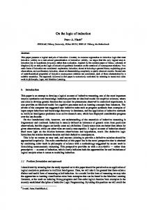
CMSC 310 Artificial Intelligence Bayesian Belief Networks 1. Definition Joint probability distribution can answer any question about the domain, but there are two major difficulties: It becomes very large as the number of variables grow. The space and time complexity is O(d n) where n is the number of random variables and d is the maximum number of values per variable Computing the probability of each atomic event may be difficult unless a large amount of data is available to derive statistical estimates. Bayesian belief networks are compact representations of joint probability distribution over a set of random variables, X1, . . . , Xn, that make use of conditional dependence and independence among the random variables. A Bayesian network specification has two components: (i) a directed acyclic graph G = (V,E) with a node set V corresponding to the random variables X1, . . . ,Xn, and edge set E on these nodes. The edges reflect conditional independence assumptions made. A node is conditionally independent of all other nodes given its parents in the network. (ii) a set of conditional probability distributions for each node in the graph G. These probability distributions are local, and are of the form P(Xi|ParentsG (Xi)). The two components (G, ) specify a unique distribution on the random variables X1, . . . ,Xn. P(X1, . . . ,Xn) = (Xi|ParentsG (Xi)), i = 1 to n. Bayesian networks contain quantitative information in the form of conditional probabilities of variables given their parents in the network. 2. Example (from Ben Coppin, Artificial Intelligence Illuminated) Consider the following Bayesian network: C S
P
E
F
1
Where the nodes represent the following statements: C = that you will go to college S = that you will study P = that you will party E = that you will be successful in your exams F = that you will have fun
If you go to college, this will affect the likelihood that you will study and the likelihood that you will party. Studying and partying affect your chances of exam success, and partying affects your chances of having fun. Conditional probability tables: P(C) 0.2 C
P(S)
true
0.8
false
0.2
C
P(P)
true
0.6
false
0.5
S
P
P(E)
true
true
0.6
true
false
0.9
false
true
0.1
false
false
0.2
P
P(F)
true
0.9
false
0.7
2
Note that there is a dependence between F and c, but it is not a direct dependence, so no information is stored about it. These conditional probability tables give us all the information necessary to carry out any reasoning about the domain. Example 1: Compute the probability that you will go to college, you will study and be successful in your exams, but you will not party or have fun: P(C = true, S = true, P = false, E = true, F = false) To simplify the notation, we will use P(C, S, ~P, E, ~F) To compute P(C, S, ~P, E, ~F), we use the rule P(X1, . . . ,Xn) = (Xi|ParentsG (Xi)), i = 1 to n. P(C, S, ~P, E, ~F) = P(C) * P(S|C) * P(~P | C) * P(E | S ~P) * P(~F | ~P) = = 0.2 * 0.8 * 0.4 * 0.9 * 0.3 = 0.01728
Example 2: Compute the probability that you will have success in your exams if you have fun and study at college, but don’t party: P( E | F , S, C, ~P) In the network, E is dependent only on S and P, so we can drop C and F From the table for P(E) we obtain P(E | S, ~P) = 0.9 Example 3: Let’s say we know that you had fun and studied hard while at college, and that you succeeded in your exams, but we don’t know whether you partied or not. Thus, we know C, S, E, and F, we don’t know P. We want to determine the most likely value for P. We can compare the values of the following two expressions: P(C, S, P, E, F) and P(C, S, ~P, E, F) P(C, S, P, E, F) = P(C) * P(S | C) * P(P | C) * P (E | S, P), * P (F | P) = = 0.2 * 0.8 * 0.6 * 0.6 * 0.9 = 0.05184 P(C, S, ~P, E, F) = P(C) * P(S | C) * P(~P | C) * P (E | S, ~P), * P (F | ~P) = = 0.2 * 0.8 * 0.4 * 0.9 * 0.7 = 0.04032 So it is slightly more likely that you did party while at college than that you didn’t.
3
3. Constructing Bayesian belief networks If we know the causal relations between events, we can build partial networks and then combine them in one network. The result should be directed acyclic graph. If we don’t know the causal relations, but we do know some of the joint probability distribution, we can use algorithms that learn Bayesian networks, e.g. genetic algorithms. Here we are looking the network that best matches (explains) the observations. This is a research topic - there is a large number of publications on building Bayesian belief networks, and there are also some commercially available systems. https://www.cra.com/pdf/bnetbuilderbackground.pdf 4. Applications Bayesian belief networks represent models of probabilistic causal relations in partially observable domains. They are very useful as a reasoning tool in expert systems and decision support systems, especially in domains where uncertainty is inherent, e.g. weather prediction, medical expert systems, business intelligence systems, risk management systems, etc. Additional Readings: https://www.cra.com/pdf/bnetbuilderbackground.pdf http://www.eecs.qmul.ac.uk/~norman/BBNs/BBNs.htm
4