1 Convex Functions on Intervals

1 Convex Functions on Intervals

The study of convex functions begins in the context of real-valued functions of a real variable. Here we find a rich variety of results with significant applications. More importantly, they will serve as a model for deep generalizations in the setting of several variables.

1.1 Convex Functions at First Glance Throughout this book I will denote a nondegenerate interval. Definition 1.1.1 A function f : I → R is called convex if f ((1 − λ)x + λy) ≤ (1 − λ)f (x) + λf (y)

(1.1)

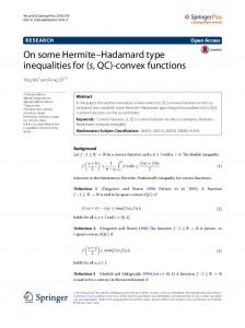
for all points x and y in I and all λ ∈ [0, 1]. It is called strictly convex if the inequality (1.1) holds strictly whenever x and y are distinct points and λ ∈ (0, 1). If −f is convex (respectively, strictly convex) then we say that f is concave (respectively, strictly concave). If f is both convex and concave, then f is said to be affine. The affine functions on intervals are precisely the functions of the form mx + n, for suitable constants m and n. One can easily prove that the following three functions are convex (though not strictly convex): the positive part x+ , the negative part x− , and the absolute value |x|. Together with the affine functions they provide the building blocks for the entire class of convex functions on intervals. See Theorem 1.5.7. The convexity of a function f : I → R means geometrically that the points of the graph of f |[u,v] are under (or on) the chord joining the endpoints (u, f (u)) and (v, f (v)), for all u, v ∈ I, u < v; see Fig. 1.1. Then f (x) ≤ f (u) +

f (v) − f (u) (x − u) v−u

(1.2)

8


for all x ∈ [u, v], and all u, v ∈ I, u < v. This shows that the convex functions are locally (that is, on any compact subinterval) majorized by affine functions. A companion result, concerning the existence of lines of support, will be presented in Section 1.5.

Fig. 1.1. Convex function: the graph is under the chord.

The intervals are closed under arbitrary convex combinations, that is, n

λk xk ∈ I

k=1

n for all x1 , . . . , xn ∈ I, and all λ1 , . . . , λn ∈ [0, 1] with k=1 λk = 1. This can be proved by induction on the number n of points involved in the convex combinations. The case n = 1 is trivial, while for n = 2 it follows from the definition of a convex set. Assuming the result is true for all convex combinations with at most n≥ 2 points, let us pass to the case of combinations n+1 with n + 1 points, x = k=1 λk xk . The nontrivial case is when all coefficients λk lie in (0, 1). But in this case, due to our induction hypothesis, x can be represented as a convex combination of two elements of I, n

x = (1 − λn+1 )

k=1

λk xk + λn+1 xn+1 , 1 − λn+1

hence x belongs to I. The above remark has a notable counterpart for convex functions: Lemma 1.1.2 (The discrete case of Jensen’s inequality) A real-valued function f defined on an interval I is convexif and only if for all x1 , . . . , xn n in I and all scalars λ1 , . . . , λn in [0, 1] with k=1 λk = 1 we have f

n k=1

n λk xk ≤ λk f (xk ). k=1

1.1 Convex Functions at First Glance

9

The above inequality is strict if f is strictly convex, all the points xk are distinct and all scalars λk are positive. A nice mechanical interpretation of this result was proposed by T. Needham [174]. The precision of Jensen’s inequality is discussed in Section 1.4. See also Exercise 7, at the end of Section 1.8. Related to the above geometrical interpretation of convexity is the following result due to S. Saks [219]: Theorem 1.1.3 Let f be a real-valued function defined on an interval I. Then f is convex if and only if for every compact subinterval J of I, and every affine function L, the supremum of f + L on J is attained at an endpoint. This statement remains valid if the perturbations L are supposed to be linear (that is, of the form L(x) = mx for suitable m ∈ R). Proof. Necessity: If f is convex, so is the sum F = f + L. Since every point of a subinterval J = [x, y] is a convex combination z = (1 − λ)x + λy of x and y, we have sup F (z) = sup F ((1 − λ)x + λy) z∈J

λ∈[0,1]

≤ sup [(1 − λ)F (x) + λF (y)] = max{F (x), F (y)}. λ∈[0,1]

Sufficiency: Given a compact subinterval J = [x, y] of I, there exists an affine function L(x) = mx + n which agrees with f at the two endpoints x and y. Then sup [(f − L)((1 − λ)x + λy)] = 0, λ∈[0,1]

which yields 0 ≥ f ((1 − λ)x + λy) − L((1 − λ)x + λy) = f ((1 − λ)x + λy) − (1 − λ)L(x) − λL(y) = f ((1 − λ)x + λy) − (1 − λ)f (x) − λf (y) for every λ ∈ [0, 1].

An easy consequence of Theorem 1.1.3 is that a convex function f is bounded on every compact subinterval [u, v] of its interval of definition. In fact, f (x) ≤ M = max{f (u), f (v)} on [u, v] and writing an arbitrary point x ∈ [u, v] in the form x = (u + v)/2 + t for some t with |t| ≤ (v − u)/2, we easily infer that u + v u + v u + v + t ≥ 2f −f −t f (x) = f 2 2 2 u + v − M. ≥ 2f 2

10


Checking that a function is convex or not is not very easy, but fortunately several useful criteria are available. Probably the simplest one is the following: Theorem 1.1.4 (J. L. W. V. Jensen [115]) Let f : I → R be a continuous function. Then f is convex if and only if f is midpoint convex, that is, f

x + y 2

≤

f (x) + f (y) 2

for all x, y ∈ I.

Proof. Clearly, only the sufficiency part needs an argument. By reductio ad absurdum, if f is not convex, then there exists a subinterval [a, b] such that the graph of f |[a,b] is not under the chord joining (a, f (a)) and (b, f (b)); that is, the function ϕ(x) = f (x) −

f (b) − f (a) (x − a) − f (a), b−a

x ∈ [a, b]

verifies γ = sup{ϕ(x) | x ∈ [a, b]} > 0. Notice that ϕ is continuous and ϕ(a) = ϕ(b) = 0. Also, a direct computation shows that ϕ is also midpoint convex. Put c = inf{x ∈ [a, b] | ϕ(x) = γ}; then necessarily ϕ(c) = γ and c ∈ (a, b). By the definition of c, for every h > 0 for which c ± h ∈ (a, b) we have ϕ(c − h) < ϕ(c) and ϕ(c + h) ≤ ϕ(c) so that

ϕ(c − h) + ϕ(c + h) 2 in contradiction with the fact that ϕ is midpoint convex. ϕ(c) >

Corollary 1.1.5 Let f : I → R be a continuous function. Then f is convex if and only if f (x + h) + f (x − h) − 2f (x) ≥ 0 for all x ∈ I and all h > 0 such that both x + h and x − h are in I. Notice that both Theorem 1.1.4 and its Corollary 1.1.5 above have straightforward variants for the case of strictly convex functions. Corollary 1.1.5 allows us to check immediately the strict convexity of some very common functions, such as the exponential function. Indeed, due to the fact that a+b √ a, b > 0, a = b, implies > ab 2 we have ex+h + ex−h − 2ex > 0 for all x ∈ R and all h > 0. An immediate consequence of this remark is the following result, which extends the well-known arithmetic mean–geometric mean inequality (abbreviated, AM–GM inequality):


11

Theorem 1.1.6 (The weighted form of the AM–GM inequality; L. J. Rogers [215]) If x1 , . . . , xn ∈ (0, ∞) and λ1 , . . . , λn ∈ (0, 1), n k=1 λk = 1, then n λk xk > xλ1 1 · · · xλnn k=1

unless x1 = · · · = xn . Replacing xk by 1/xk in the last inequality we get (under the same hypotheses on xk and λk ), xλ1 1 · · · xλnn > 1 /

n λk xk

k=1

unless x1 = · · · = xn (which represents the weighted form of the geometric mean–harmonic mean inequality). The particular case of Theorem 1.1.6 where λ1 = · · · = λn = 1/n represents the usual AM–GM inequality, which can be completed as above, with its relation to the harmonic mean: For every family x1 , . . . , xn of positive numbers we have √ x1 + · · · + xn n > n x1 · · · xn > 1 1 n + · · · + x1 xn unless x1 = · · · = xn . An estimate of these inequalities is the objective of Section 2.5 below. The closure under functional operations with convex functions is an important source of examples in this area. Proposition 1.1.7 (The operations with convex functions) (i) Adding two convex functions (defined on the same interval) we obtain a convex function; if one of them is strictly convex, then the sum is also strictly convex. (ii) Multiplying a (strictly) convex function by a positive scalar we obtain also a (strictly) convex function. (iii) The restriction of every (strictly) convex function to a subinterval of its domain is also a (strictly) convex function. (iv) If f : I → R is a convex (respectively a strictly convex) function and g : R → R is a nondecreasing (respectively an increasing) convex function, then g ◦ f is convex (respectively strictly convex). (v) Suppose that f is a bijection between two intervals I and J. If f is increasing, then f is (strictly) convex if and only if f −1 is (strictly) concave. If f is a decreasing bijection, then f and f −1 are of the same type of convexity. We end this section with an analogue of Theorem 1.1.4 for triplets:

12


Theorem 1.1.8 (Popoviciu’s inequality [206]) Let f : I → R be a continuous function. Then f is convex if and only if x + y + z f (x) + f (y) + f (z) +f 3 3 y + z z + x 2 x + y +f +f ≥ f 3 2 2 2 for all x, y, z ∈ I. In the variant of strictly convex functions the above inequality is strict except for x = y = z. Proof. Necessity: (this implication does not need the assumption on continuity). Without loss of generality we may assume that x ≤ y ≤ z. If y ≤ (x + y + z)/3, then (x + y + z)/3 ≤ (x + z)/2 ≤ z

and

(x + y + z)/3 ≤ (y + z)/2 ≤ z,

which yields two numbers s, t ∈ [0, 1] such that x+z x+y+z =s· + (1 − s) · z 2 3 y+z x+y+z =t· + (1 − t) · z. 2 3 Summing up, we get (x + y − 2z)(s + t − 3/2) = 0. If x + y − 2z = 0, then necessarily x = y = z, and Popoviciu’s inequality is clear. If s + t = 3/2, we have to sum up the following three inequalities: x + z x + y + z f ≤s·f + (1 − s) · f (z) 2 3 x + y + z y + z ≤t·f + (1 − t) · f (z) f 2 3 x + y 1 1 ≤ · f (x) + · f (y) f 2 2 2 and then multiply both sides by 2/3. The case where (x + y + z)/3 < y can be treated in a similar way. Sufficiency: Popoviciu’s inequality (when applied for y = z), yields the following substitute for the condition of midpoint convexity: x + y 1 3 x + 2y f (x) + f ≥f for all x, y ∈ I. (1.3) 4 4 3 2 Using this remark, the proof follows verbatim the argument of Theorem 1.1.4 above. The above statement of Popoviciu’s inequality is only a simplified version of a considerably more general result; see the Comments at the end of this chapter. However, even this version leads to interesting inequalities; see Exercise 9. An estimate from below of Popoviciu’s inequality is available in [188].


13

Exercises 1. Prove that the following functions are strictly convex: • • •

− log x and x log x on (0, ∞); xp on [0, ∞) if p > 1; xp on (0, ∞) if p < 0; −xp on [0, ∞) if p ∈ (0, 1); (1 + xp )1/p on [0, ∞) if p > 1.

2. Let f : I → R be a convex function and let x1 , . . . , xn ∈ I (n ≥ 2). Prove that f (x ) + · · · + f (x x + · · · + x 1 n−1 ) 1 n−1 (n − 1) −f n−1 n−1 cannot exceed x + · · · + x f (x ) + · · · + f (x ) 1 n 1 n −f . n n n 3. Let x1 , . . . , xn > 0 (n ≥ 2) and for each 1 ≤ k ≤ n put Ak = (i)

x1 + · · · + xk k

(T. Popoviciu) Prove that A n n

Gn (ii)

and Gk = (x1 · · · xk )1/k .

≥

A

n−1

n−1

Gn−1

≥ ··· ≥

A 1 1

G1

= 1.

(R. Rado) Prove that n(An − Gn ) ≥ (n − 1)(An−1 − Gn−1 ) ≥ · · · ≥ 1 · (A1 − G1 ) = 0.

[Hint: Apply the result of Exercise 2 to f = − log and respectively to f = exp.] 4. Suppose that f1 , . . . , fn are nonnegative concave functions with the same domain of definition. Prove that (f1 · · · fn )1/n is also a concave function. 5. (i)

(ii)

Prove that Theorem 1.1.4 remains true if the condition of midpoint convexity is replaced by: f ((1 − α)x + αy) ≤ (1 − α)f (x) + αf (y) for some fixed parameter α ∈ (0, 1), and for all x, y ∈ I. Prove that Theorem 1.1.4 remains true if the condition of continuity is replaced by boundedness from above on every compact subinterval.

6. (New from old) Assume that f (x) is a (strictly) convex function for x > 0. Prove that xf (1/x) is (strictly) convex too. √ 7. Infer from Theorem 1.1.6 that min (x + y + x12 y ) = 4/ 2. x,y>0

8. (The power means in the discrete case: see Section 1.8, Exercise 1, for the integral case.) Let x = (x1 , . . . , xn ) and α = (α1 , . . . , αn ) be two n-tuples

14


of positive elements, such that of order t is defined as Mt (x; α) =

n k=1

n

αk = 1. The (weighted) power mean

αk xtk

1/t

for t = 0

k=1

and M0 (x; α) = lim Mt (x, α) = t→0+

n

k xα k .

k=1

Notice that M1 is the arithmetic mean, M0 is the geometric mean and M−1 is the harmonic mean. Moreover, M−t (x; α) = Mt (x−1 ; α)−1 . (i) Apply Jensen’s inequality to the function xt/s , to prove that s≤t

implies Ms (x; α) ≤ Mt (x; α).

(ii) Prove that the function t → t log Mt (x; α) is convex on R. (iii) We define M−∞ (x; α) = inf{xk | k} and M∞ (x, α) = sup{xk | k}. Prove that lim Mt (x; α) = M−∞ (x; α)

t→−∞

and

lim Mt (x; α) = M∞ (x; α).

t→∞

9. (An illustration of Popoviciu’s inequality) Suppose that x1 , x2 , x3 are positive numbers, not all equal. Prove that: (i) 27 i 64x1 x2 x3 (x1 + x2 + x3 )3 ; (ii)

x61 + x62 + x63 + 3x21 x22 x23 > 2(x31 x32 + x32 x33 + x33 x31 ).

1.2 Young’s Inequality and Its Consequences Young’s inequality asserts that ab ≤

ap bq + p q

for all a, b ≥ 0,

whenever p, q ∈ (1, ∞) and 1/p + 1/q = 1; the equality holds if and only if ap = bq . This is a consequence of the strict convexity of the exponential function. In fact, p

q

ab = elog ab = e(1/p) log a +(1/q) log b p q bq 1 1 ap + < elog a + elog b = p q p q for all a, b > 0 with ap = bq . An alternative argument can be obtained by studying the variation of the function

1.2 Young’s Inequality and Its Consequences

F (a) =

bq ap + − ab, p q

15

a ≥ 0,

where b ≥ 0 is a parameter. Then F has a strict global minimum at a = bq/p , which yields F (a) > F (bq/p ) = 0 for all a ≥ 0, a = bq/p . W. H. Young [247] actually proved a much more general inequality which yields the aforementioned one for f (x) = xp−1 : Theorem 1.2.1 (Young’s inequality) Suppose that f : [0, ∞) → [0, ∞) is an increasing continuous function such that f (0) = 0 and limx→∞ f (x) = ∞. Then a

ab ≤

b

f (x) dx + 0

f −1 (x) dx

0

for all a, b ≥ 0, and equality occurs if and only if b = f (a). Proof. Using the definition of the derivative we can easily prove that the function x f (x) F (x) = f (t) dt + f −1 (t) dt − xf (x) 0

0

is differentiable, with F identically 0. This yields u f (t) dt + 0 ≤ u ≤ a and 0 ≤ v ≤ f (a) =⇒ uv ≤ 0

and the conclusion of the theorem is now clear.

v

f −1 (t) dt

0

Fig. 1.2. The areas of the two curvilinear triangles exceed the area of the rectangle with sides u and v.

The geometric meaning of Young’s inequality is indicated in Fig. 1.2. Young’s inequality is the source of many basic inequalities. The next two applications concern complex functions defined on an arbitrary measure space (X, Σ, µ).

16


Theorem 1.2.2 (The Rogers–H¨ older inequality for p > 1) Let p, q ∈ (1, ∞) with 1/p + 1/q = 1, and let f ∈ Lp (µ) and g ∈ Lq (µ). Then f g is in L1 (µ) and we have f g dµ ≤ |f g| dµ (1.4) X

X

and

|f g| dµ ≤ f Lp gLq

(1.5)

X

f g dµ ≤ f Lp gLq .

and thus

(1.6)

X

The above result extends in a straightforward manner to the pairs p = 1, q = ∞ and p = ∞, q = 1. In the complementary domain, p ∈ (−∞, 1)\{0} and 1/p + 1/q = 1, the inequality sign in (1.4)–(1.6) should be reversed. See Exercises 3 and 4. For p = q = 2, the inequality (1.6) is called the Cauchy–Buniakovski– Schwarz inequality. Proof. The first inequality is trivial. If f or g is zero µ-almost everywhere, then the second inequality is trivial. Otherwise, using Young’s inequality, we have |f (x)| |g(x)| 1 |f (x)|p 1 |g(x)|q · ≤ · + · p f Lp gLq p f Lp q gqLq for all x in X, such that f g ∈ L1 (µ). Thus 1 |f g| dµ ≤ 1 f Lp gLq X and this proves (1.5). The inequality (1.6) is immediate.

Remark 1.2.3 (Conditions for equality in Theorem 1.2.2) The basic observation is the fact that f dµ = 0 imply f = 0 µ-almost everywhere. f ≥ 0 and X

Consequently we have equality in (1.4) if and only if f (x)g(x) = eiθ |f (x)g(x)| for some real constant θ and for µ-almost every x. Suppose that p, q ∈ (1, ∞) and f and g are not zero µ-almost everywhere. In order to get equality in (1.5) it is necessary and sufficient to have |f (x)| |g(x)| 1 |f (x)|p 1 |g(x)|q · = · + · p f Lp gLq p f Lp q gqLq

1.2 Young’s Inequality and Its Consequences

17

almost everywhere. The equality case in Young’s inequality shows that this is equivalent to |f (x)|p /f pLp = |g(x)|q /gqLq almost everywhere, that is, A|f (x)|p = B|g(x)|q

almost everywhere

for some nonnegative numbers A and B. If p = 1 and q = ∞, we have equality in (1.5) if and only if there is a constant λ ≥ 0 such that |g(x)| ≤ λ almost everywhere, and |g(x)| = λ for almost every point where f (x) = 0. Theorem 1.2.4 (Minkowski’s inequality) For 1 ≤ p < ∞ and f, g ∈ Lp (µ) we have f + gLp ≤ f Lp + gLp . (1.7) In the discrete case, using the notation of Exercise 8 in Section 1.1, this inequality reads Mp (x + y, α) ≤ Mp (x, α) + Mp (y, α).

(1.8)

In this form, it extends to the complementary range 0 < p < 1, with the inequality sign reversed. The integral analogue for p < 1 is presented in Section 3.6. Proof. For p = 1, the inequality (1.7) follows immediately by integrating the inequality |f + g| ≤ |f | + |g|. For p ∈ (1, ∞) we have |f + g|p ≤ (|f | + |g|)p ≤ (2 sup{|f |, |g|})p ≤ 2p (|f |p + |g|p ), which shows that f + g ∈ Lp (µ). Moreover, according to Theorem 1.2.2, |f + g|p dµ ≤ |f + g|p−1 |f | dµ + |f + g|p−1 |g| dµ f + gpLp = X

X

X

1/p

|f |p dµ

≤

|f + g|(p−1)q dµ

X

X 1/p

|g| dµ p

+

1/q

X

= (f Lp + gLp )f +

1/q |f + g|

(p−1)q

dµ

X p/q gLp ,

where 1/p + 1/q = 1, and it remains to observe that p − p/q = 1.

Remark 1.2.5 If p = 1, we obtain equality in (1.7) if and only if there is a positive measurable function ϕ such that f (x)ϕ(x) = g(x) almost everywhere on the set {x | f (x)g(x) = 0}. If p ∈ (1, ∞) and f is not 0 almost everywhere, then we have equality in (1.7) if and only if g = λf almost everywhere, for some λ ≥ 0.

18


In the particular case when (X, Σ, µ) is the measure space associated with the counting measure on a finite set, µ : P({1, . . . , n}) → N,

µ(A) = |A|,

we retrieve the classical discrete forms of the above inequalities. For example, the discrete version of the Rogers–Hölder inequality can be read n n n 1/p 1/q ξk ηk ≤ |ξk |p |ηk |q k=1

k=1

k=1

for all ξk , ηk ∈ C, k ∈ {1, . . . , n}. On the other hand, a moment’s reflection shows that we can pass immediately from these discrete inequalities to their integral analogues, corresponding to finite measure spaces. Remark 1.2.6 It is important to notice that all numerical inequalities of the form f (x1 , . . . , xn ) ≥ 0 for x1 , . . . , xn ≥ 0 (1.9) where f is a continuous and positively homogeneous function of degree 1 (that is, f (λx1 , . . . , λxn ) = λf (x1 , . . . , xn ) for λ ≥ 0), extend to the context of Banach lattices, via a functional calculus invented by A. J. Yudin and J. L. Krivine. This allows us to replace the real variables of f by positive elements of a Banach lattice. See [147, Vol. 2, pp. 40–43]. Particularly, this is the case of the AM–GM inequality, Rogers–H¨ older’s inequality, and Minkowski’s inequality. Also, all numerical inequalities of the form (1.9), attached to continuous functions, extend (via the functional calculus with self-adjoint elements) to the context of C ∗ -algebras. In fact, the n-tuples of real numbers can be replaced by n-tuples of mutually commuting positive elements of a C ∗ -algebra. See [58].

Exercises 1. Recall the identity of Lagrange, n k=1

a2k

n

b2k =

k=1

(aj bk − ak bj )2 +

1≤j −1 we have (1 + x)α ≥ 1 + αx if α ∈ (−∞, 0] ∪ [1, ∞) and (1 + x)α ≤ 1 + αx if α ∈ [0, 1]; (ii)

if α ∈ / {0, 1}, the equality occurs only for x = 0. The substitution 1 + x → x/y followed by a multiplication by y leads us to Young’s inequality (for full range of parameters). Show that this inequality can be written xy ≥

xp yq + p q

for all x, y > 0

in the domain p ∈ (−∞, 1)\{0} and 1/p + 1/q = 1. 3. (The Rogers–Hölder inequality for p ∈ (−∞, 1)\{0} and 1/p + 1/q = 1) Apply Young’s inequality to prove that n

|ak bk | ≥

k=1

n

|ak |p

k=1

n 1/p

|bk |q

1/q

k=1

for all a1 , . . . , an , b1 , . . . , bn ∈ C and all n ∈ N∗ . 4. (A symmetric form of Rogers–H¨ older inequality) Let p, q, r be nonzero real numbers such that 1/p + 1/q = 1/r. (i) Prove that the inequality n

λk |ak bk |r

1/r

k=1

≤

n

λk |ak |p

n 1/p

k=1

λk |bk |q

1/q

k=1

holds in each of the following three cases: p > 0, q > 0, r > 0; (ii)

p < 0, q > 0, r < 0;

p > 0, q < 0, r < 0.

Prove that the opposite inequality holds in each of the following cases: p > 0, q < 0, r > 0;

p < 0, q > 0, r > 0; p < 0, q < 0, r < 0. n > 0, k=1 λk = 1, and a1 , . . . , an , b1 , . . . , bn ∈

Here λ1 , . . . , λn C\{0}, n ∈ N∗ . (iii) Formulate the above inequalities in terms of power means and then prove they still work for r = pq/(p + q) if p and q are not both zero, and r = 0 if p = q = 0.

20


5. Prove the following generalization of the Rogers–H¨ older inequality: If (X, Σ, µ) is a measure space and f1 , . . . , fn are functions such that fk ∈ n Lpk (µ) for some pk ≥ 1, and k=1 1/pk = 1, then n n dµ ≤ f fk Lpk . k X

k=1

k=1

6. (A general form of Minkowski’s inequality, see [144, p. 47]) Suppose that (X, M, µ) and (Y, N , ν) are two σ-finite measure spaces, f is a nonnegative function on X × Y which is µ × ν-measurable, and let p ∈ [1, ∞). Then

p f (x, y) dν(y)

X

1/p dµ(x)

Y

≤

1/p p

f (x, y) dµ(x) Y

dν(y).

X

1.3 Smoothness Properties The entire discussion on the smoothness properties of convex functions on intervals is based on their characterization in terms of slopes of variable chords through arbitrary fixed points of their graphs. Given a function f : I → R and a point a ∈ I, one can associate with them a new function, sa : I\{a} → R,

sa (x) =

f (x) − f (a) , x−a

whose value at x is the slope of the chord joining the points (a, f (a)) and (x, f (x)) of the graph of f . Theorem 1.3.1 (L. Galvani [86]) Let f be a real function defined on an interval I. Then f is convex (respectively, strictly convex) if and only if the associated functions sa are nondecreasing (respectively, increasing). In fact,

1 x f (x) 1 x x2 sa (y) − sa (x) 1 y y 2 = 1 y f (y) y−x 1 a f (a) 1 a a2

for all three distinct points a, x, y of I, and the proof of Theorem 1.3.1 is a consequence of the following lemma: Lemma 1.3.2 Let f be a real function defined on an interval I. Then f is convex if and only if 1 x f (x) 1 x x2 1 y f (y) 1 y y 2 ≥ 0 1 z z 2 1 z f (z) for all three distinct points x, y, z of I; equivalently, if and only if

1.3 Smoothness Properties

1 x f (x) 1 y f (y) ≥ 0 1 z f (z)

21

(1.10)

for all x < y < z in I. The corresponding variant for strict convexity is valid too, provided that ≥ is replaced by >. Proof. The condition (1.10) means that (z − y)f (x) − (z − x)f (y) + (y − x)f (z) ≥ 0 for all x < y < z in I. Since each y between x and z can be written as y = (1 − λ)x + λz, the latter condition is equivalent to the assertion that f ((1 − λ)x + λz) ≤ (1 − λ)f (x) + λf (z) for all x < z in I and all λ ∈ [0, 1].

We are now prepared to state the main result on the smoothness of convex functions. Theorem 1.3.3 (O. Stolz [233]) Let f : I → R be a convex function. Then f is continuous on the interior int I of I and has finite left and right derivatives at each point of int I. Moreover, x < y in int I implies (x) ≤ f+ (x) ≤ f− (y) ≤ f+ (y). f− Particularly, both f− and f+ are nondecreasing on int I.

Proof. In fact, according to Theorem 1.3.1 above, we have f (x) − f (a) f (y) − f (a) f (z) − f (a) ≤ ≤ x−a y−a z−a for all x ≤ y < a < z in I. This fact assures us that the left derivative at a exists and f (z) − f (a) f− . (a) ≤ z−a A symmetric argument will then yield the existence of f+ (a) and the availability of the relation f− (a) ≤ f+ (a). On the other hand, starting with x < u ≤ v < y in int I, the same Theorem 1.3.1 yields

f (u) − f (x) f (v) − f (x) f (v) − f (y) ≤ ≤ , u−x v−x v−y so letting u → x+ and v → y−, we obtain that f+ (x) ≤ f− (y).

22


Because f admits finite lateral derivatives at each interior point, it will be continuous at each interior point. By Theorem 1.3.3, every continuous convex function f (defined on a non (a) and f− (b) at the degenerate compact interval [a, b]) admits derivatives f+ endpoints, but they can be infinite, −∞ ≤ f+ (a) < ∞

and

− ∞ < f− (b) ≤ ∞.

How nondifferentiable can a convex function be? Due to Theorem 1.3.3 above, we can immediately prove that every convex function f : I → R is differentiable except for an enumerable subset. In fact, by considering the set Ind = {x | f− (x) < f+ (x)} and letting for each x ∈ Ind a rational point rx ∈ (f− (x), f+ (x)) we get a one-to-one function ϕ : x → rx from Ind into Q. Consequently, Ind is at most countable. Notice that this reasoning depends on the axiom of choice. An example of a convex function which is not differentiable on a dense countable set will be exhibited in Remark 1.6.2 below. See also Exercise 3 at the end of this section. Simple examples such as f (x) = 0 if x ∈ (0, 1), and f (0) = f (1) = 1, show that upward jumps could appear at the endpoints of the interval of definition of a convex function. Fortunately, the possible discontinuities are removable:

Proposition 1.3.4 If f : [a, b] → R is f (b−) exist in R and ⎧ ⎪ ⎨f (a+) f (x) = f (x) ⎪ ⎩ f (b−)

a convex function, then f (a+) and if x = a if x ∈ (a, b) if x = b

is convex too. This result is a consequence of the following: Proposition 1.3.5 If f : I → R is convex, then either f is monotonic on int I, or there exists an ξ ∈ int I such that f is nonincreasing on the interval (−∞, ξ] ∩ I and nondecreasing on the interval [ξ, ∞) ∩ I. Proof. Since any convex function verifies formulas of the type (1.2), it suffices to consider the case where I is open. If f is not monotonic, then there must exist points a < b < c in I such that f (a) > f (b) < f (c). The other possibility, f (a) < f (b) > f (c), is rejected by the same formula (1.2). Since f is continuous on [a, c], it attains its infimum on this interval at a point ξ ∈ [a, c], that is,


23

f (ξ) = inf f ([a, c]). Actually, f (ξ) = inf f (I). In fact, if x < a, then according to Theorem 1.3.1 we have f (x) − f (ξ) f (a) − f (ξ) ≤ , x−ξ a−ξ which yields (ξ − a)f (x) ≥ (x − a)f (ξ) + (ξ − x)f (a) ≥ (ξ − a)f (ξ), that is, f (x) ≥ f (ξ). The other case, when c < x, can be treated in a similar manner. If u < v < ξ, then su (ξ) = sξ (u) ≤ sξ (v) =

f (v) − f (ξ) ≤0 v−ξ

and thus su (v) ≤ su (ξ) ≤ 0. This shows that f is nonincreasing on I ∩(−∞, ξ]. Analogously, if ξ < u < v, then from sv (ξ) ≤ sv (u) we infer that f (v) ≥ f (u), hence f is nondecreasing on I ∩ [ξ, ∞). Corollary 1.3.6 Every convex function f : I → R which is not monotonic on int I has an interior global minimum. There is another way to look at the smoothness properties of the convex functions, based on the Lipschitz condition. A function f defined on an interval J is said to be Lipschitz if there exists a constant L ≥ 0 such that |f (x) − f (y)| ≤ L|x − y|

for all x, y ∈ J.

A famous result due to H. Rademacher asserts that any Lipschitz function is differentiable almost everywhere. See Theorem 3.11.1. Theorem 1.3.7 If f : I → R is a convex function, then f is Lipschitz on any compact interval [a, b] contained in the interior of I. Proof. By Theorem 1.3.3, f+ (a) ≤ f+ (x) ≤

f (y) − f (x) ≤ f− (y) ≤ f− (b) y−x

for all x, y ∈ [a, b] with x < y, hence f |[a,b] verifies the Lipschitz condition (a)|, |f− (b)|}. with L = max{|f+ Corollary 1.3.8 If fn : I → R (n ∈ N) is a pointwise converging sequence of convex functions, then its limit f is also convex. Moreover, the convergence is uniform on any compact subinterval included in int I, and (fn )n converges to f except possibly at countably many points of I.

24


Since the first derivative of a convex function may not exist at a dense subset, a characterization of convexity in terms of second order derivatives is not possible unless we relax the concept of twice differentiability. The upper and the lower second symmetric derivative of f at x, are respectively defined by the formulas D f (x) = lim sup

f (x + h) + f (x − h) − 2f (x) h2

D2 f (x) = lim inf

f (x + h) + f (x − h) − 2f (x) . h2

2

h↓0

h↓0

It is not difficult to check that if f is twice differentiable at a point x, then 2

D f (x) = D2 f (x) = f (x); 2

however D f (x) and D2 f (x) can exist even at points of discontinuity; for example, consider the case of the signum function and the point x = 0. Theorem 1.3.9 Suppose that I is an open interval. A real-valued function f 2 is convex on I if and only if f is continuous and D f ≥ 0. Accordingly, if a function f : I → R is convex in the neighborhood of each point of I, then it is convex on the whole interval I. 2

Proof. If f is convex, then clearly D f ≥ D2 f ≥ 0. The continuity of f follows from Theorem 1.3.3. 2 Now, suppose that D f > 0 on I. If f is not convex, then we can find a 2 point x0 such that D f (x0 ) ≤ 0, which will be a contradiction. In fact, in this case there exists a subinterval I0 = [a0 , b0 ] such that f ((a0 +b0 )/2) > (f (a0 )+ f (b0 ))/2. A moment’s reflection shows that one of the intervals [a0 , (a0 +b0 )/2], [(3a0 + b0 )/4, (a0 + 3b0 )/4], [(a0 + b0 )/2, b0 ] can be chosen to replace I0 by a smaller interval I1 = [a1 , b1 ], with b1 − a1 = (b0 − a0 )/2 and f ((a1 + b1 )/2) > (f (a1 ) + f (b1 ))/2. Proceeding by induction, we arrive at a situation where the principle of included intervals gives us the point x0 . In the general case, consider the sequence of functions fn (x) = f (x) +

1 2 x . n

2

Then D fn > 0, and the above reasoning shows us that fn is convex. Clearly fn (x) → f (x) for each x ∈ I, so that the convexity of f will be a consequence of Corollary 1.3.8 above. Corollary 1.3.10 (The second derivative test) Suppose that f : I → R is a twice differentiable function. Then: (i) f is convex if and only if f ≥ 0;


(ii)

25

f is strictly convex if and only if f ≥ 0 and the set of points where f vanishes does not include intervals of positive length.

An important result due to A. D. Alexandrov asserts that all convex functions are almost everywhere twice differentiable. See Theorem 3.11.2. Remark 1.3.11 (Higher order convexity) The following generalization of the notion of a convex function was initiated by T. Popoviciu in 1934. A function f : [a, b] → R is said to be n-convex (n ∈ N∗ ) if for all choices of n + 1 distinct points x0 < · · · < xn in [a, b], the n-th order divided difference of f satisfies f [x0 , . . . , xn ] ≥ 0. The divided differences are given inductively by f (x0 ) − f (x1 ) x0 − x1 f [x0 , x1 ] − f [x1 , x2 ] f [x0 , x1 , x2 ] = x0 − x2 .. . f [x0 , x1 ] =

f [x0 , . . . , xn ] =

f [x0 , . . . , xn−1 ] − f [x1 , . . . , xn ] . x0 − xn

Thus the 1-convex functions are the nondecreasing functions, while the 2-convex functions are precisely the classical convex functions. In fact, 1 x f (x) 1 x x2 1 y y 2 = f [y, z] − f [x, z] , 1 y f (y) y−x 1 z f (z) 1 z z 2 and the claim follows from Lemma 1.3.2. As T. Popoviciu noticed in his book [205], if f is n-times differentiable, with f (n) ≥ 0, then f is n-convex. See [196] and [212] for a more detailed account on the theory of n-convex functions.

Exercises 1. (An application of the second derivative test of convexity) (i) Prove that the functions log((eax −1)/(ex −1)) and log(sinh ax/ sinh x) are convex on R if a ≥ 1. √ √ (ii) Prove that the function b log cos(x/ b) − a log cos(x/ a) is convex on (0, π/2) if b ≥ a ≥ 1. 2. Suppose that 0 < a < b < c (or 0 < b < c < a, or 0 < c < b < a). Use Lemma 1.3.2 to infer the following inequalities:

26


abα + bcα + caα > acα + baα + cbα for α ≥ 1; ab bc ca > ac cb ba ; a(c − b) b(a − c) c(b − a) (iii) + + > 0. (c + b)(2a + b + c) (a + c)(a + 2b + c) (b + a)(a + b + 2c) ∞ n 3. Show that the function f (x) = n=0 |x − n|/2 , x ∈ R, provides an example of a convex function which is nondifferentiable on a countable subset. (i) (ii)

4. Let D be a bounded closed convex subset of the real plane. Prove that D can be always represented as D = {(x, y) | f (x) ≤ y ≤ g(x), x ∈ [a, b]} for suitable functions f : [a, b] → R convex, and g : [a, b] → R concave. Infer that the boundary of D is smooth except possibly for an enumerable subset. 5. Prove that a continuous convex function f : [a, b] → R can be extended to a convex function on R if and only if f+ (a) and f− (b) are finite. 6. Use Corollary 1.3.10 to prove that the sine function is strictly concave on [0, π]. Infer that x a cot a sin a x ≤ sin x ≤ sin a a a for every a ∈ (0, π/2] and every x ∈ [0, a]. For a = π/2 this yields the classical inequality of Jordan. 7. Let f : [0, 2π] → R be a convex function. Prove that 1 2π an = f (t) cos nt dt ≥ 0 for every n ≥ 1. π 0 8. (J. L. W. V. Jensen [115]) Prove that a function f : [0, M ] → R is nondecreasing if and only if n n n λk f (xk ) ≤ λk f xk k=1

k=1

k=1

for n all finite families λ1 , . . . , λn ≥ 0 and x1 , . . . , xn ∈ [0, M ], with k=1 xk ≤ M and n ≥ 2. This applies to any continuous convex function g : [0, M ] → R, noticing that [g(x) − g(0)]/x is nondecreasing. 9. (van der Corput’s lemma) Let λ > 0 and let f : R → R be a function of class C 2 such that f ≥ λ. Prove that b if (t) ≤ 4 2/λ for all a, b ∈ R. e dt a

[Hint: Use integration by parts on intervals around the point where f vanishes. ]

1.4 An Upper Estimate of Jensen’s Inequality

27

1.4 An Upper Estimate of Jensen’s Inequality An important topic related to inequalities is their precision. The following result (which exhibits the power of one-variable techniques in a several-variables context) yields an upper estimate of Jensen’s inequality: Theorem 1.4.1 Let f : [a, b] → R be a convex function and let [m1 , M1 ], . . . , [mn , Mn ] be compact subintervals of [a, b]. Given λ1 , . . . , λn in [0, 1], with the function E(x1 , . . . , xn ) =

n

λk f (xk ) − f

n

k=1

n k=1

λk = 1,

λk xk

k=1

attains its maximum on Ω = [m1 , M1 ] × · · · × [mn , Mn ] at a vertex, that is, at a point of {m1 , M1 } × · · · × {mn , Mn }. The proof depends upon the following refinement of Lagrange’s mean value theorem: Lemma 1.4.2 Let h : [a, b] → R be a continuous function. Then there exists a point c ∈ (a, b) such that Dh(c) ≤

h(b) − h(a) ≤ Dh(c). b−a

Here Dh(c) = lim inf x→c

h(x) − h(c) x−c

and

Dh(c) = lim sup x→c

h(x) − h(c) . x−c

are respectively the lower derivative and the upper derivative of h at c. Proof. As in the smooth case, we consider the function H(x) = h(x) −

h(b) − h(a) (x − a), b−a

x ∈ [a, b].

Clearly, H is continuous and H(a) = H(b). If H attains its supremum at c ∈ (a, b), then DH(c) ≤ 0 ≤ DH(c) and the conclusion of Lemma 1.4.2 is immediate. The same is true when H attains its infimum at an interior point of [a, b]. If both extremes are attained at the endpoints, then H is constant and the conclusion of Lemma 1.4.2 works for all c in (a, b). Proof of Theorem 1.4.1. Clearly, we may assume that f is also continuous. We shall show (by reductio ad absurdum) that

28


E(x1 , . . . , xk , . . . , xn ) ≤ sup{E(x1 , . . . , mk , . . . , xn ), E(x1 , . . . , Mk , . . . , xn )} for all (x1 , x2 , . . . , xn ) ∈ Ω and all k ∈ {1, . . . , n}. In fact, if E(x1 , x2 , . . . , xn ) > sup{E(m1 , x2 , . . . , xn ), E(M1 , x2 , . . . , xn )} for some (x1 , x2 , . . . , xn ) ∈ Ω, we consider the function h : [m1 , M1 ] → R,

h(x) = E(x, x2 , . . . , xn ).

According to Lemma 1.4.2, there exists a ξ ∈ (m1 , x1 ) such that h(x1 ) − h(m1 ) ≤ (x1 − m1 )Dh(ξ). Since h(x1 ) > h(m1 ), it follows that Dh(ξ) > 0, equivalently, Df (ξ) > Df (λ1 ξ + λ2 x2 + · · · + λn xn ). Or, Df = f+ is a nondecreasing function on (a, b), which yields

ξ > λ1 ξ + λ2 x2 + · · · + λn xn , and thus ξ > (λ2 x2 + · · · + λn xn )/(λ2 + · · · + λn ). A new appeal to Lemma 1.4.2 (applied this time to h|[x1 ,M1 ] ), yields an η ∈ (x1 , M1 ) such that η < (λ2 x2 + · · · + λn xn )/(λ2 + · · · + λn ). But this contradicts the fact that ξ < η. Corollary 1.4.3 Let f : [a, b] → R be a convex function. Then a + b f (c) + f (d) c + d f (a) + f (b) −f ≥ −f 2 2 2 2 for all a ≤ c ≤ d ≤ b. An application of Corollary 1.4.3 to series summation may be found in [99, p. 100]. Theorem 1.4.1 allows us to retrieve a remark due to L. G. Khanin [125]: n Let p > 1, x1 , . . . , xn ∈ [0, M ] and λ1 , . . . , λn ∈ [0, 1], with k=1 λk = 1. Then n n p λk xpk ≤ λk xk + (p − 1)pp/(1−p) M p . k=1

k=1

In particular, x + · · · + x 2 M 2 x21 + · · · + x2n 1 n ≤ , + n n 4 which represents an additive converse to the Cauchy–Buniakovski–Schwarz inequality. In fact, according to Theorem 1.4.1, the function n n p λk xpk − λk xk , E(x1 , . . . , xn ) = k=1 n

k=1

attains its supremum on [0, M ] at a point whose coordinates are either 0 or M . Therefore sup E(x1 , . . . , xn ) does not exceed M p ·sup {s − sp | s ∈ [0, 1]} = (p − 1) pp/(1−p) M p .

1.5 The Subdifferential

29

Exercises 1. (Kantorovich’s inequality) Let m, M, a1 , . . . , an be positive numbers, with m < M . Prove that the maximum of f (x1 , . . . , xn ) =

n

ak xk

n

k=1

ak /xk

k=1

for x1 , . . . , xn ∈ [m, M ] is equal to (M + m)2 2 (M − m)2 ak − 4M m 4M m

n

k=1

min X⊂{1,...,n}

ak −

k∈X

2 ak

.

k∈X

Remark. The following particular case n 1

n

k=1

xk

n 1 1 (M + m)2 (1 + (−1)n+1 )(M − m)2 − ≤ n xk 4M m 8M mn2 k=1

represents an improvement on Schweitzer’s inequality for odd n. 2. Let ak , bk , ck , mk , Mk , mk , Mk be positive numbers with mk < Mk and mk < Mk for k ∈ {1, . . . , n} and let p > 1. Prove that the maximum of n

ak xpk

n

k=1

bk ykp

n

k=1

p ck xk yk

k=1

for xk ∈ [mk , Mk ] and yk ∈ [mk , Mk ] (k ∈ {1, . . . , n}) is attained at a 2n-tuple whose components are endpoints. 3. Assume that f : I → R is strictly convex and continuous and g : I → R is continuous. For a1 , . . . , an > 0 and mk , Mk ∈ I, with mk < Mk for k ∈ {1, . . . , n}, consider the function h(x1 , . . . , xn ) =

n k=1

ak f (xk ) + g

n k=1

ak xk

n

ak

k=1

n

defined on k=1 [mk , Mk ]. Prove that a necessary condition for a point (y1 , . . . , yn ) to be a point of maximum is that at most one component yk is inside the corresponding interval [mk , Mk ].

1.5 The Subdifferential In the case of nonsmooth convex functions, the lack of tangent lines can be supplied by support lines. See Fig. 1.3. Given a function f : I → R, we say that f admits a support line at x ∈ I if there exists a λ ∈ R such that

30


f (y) ≥ f (x) + λ(y − x),

for all y ∈ I.

We call the set ∂f (x) of all such λ the subdifferential of f at x. Geometrically, the subdifferential gives us the slopes of the supporting lines for the graph of f . The subdifferential is always a convex set, possibly empty.

Fig. 1.3. Convexity: the existence of support lines at interior points.

The convex functions have the remarkable property that ∂f (x) = ∅ at all interior points. However, even in their case, the subdifferential could be empty at the endpoints. An example is given by the continuous convex function √ f (x) = 1 − 1 − x2 , x ∈ [−1, 1], which fails to have a support line at x = ±1. We may think of ∂f (x) as the value at x of a set-valued function ∂f (the subdifferential of f ), whose domain dom ∂f consists of all points x in I where f has a support line. Lemma 1.5.1 Let f be a convex function on an interval I. Then ∂f (x) = ∅ at all interior points of I. Moreover, every function ϕ : I → R for which ϕ(x) ∈ ∂f (x) whenever x ∈ int I verifies the double inequality (x) ≤ ϕ(x) ≤ f+ (x), f−

and thus is nondecreasing on int I. The conclusion above includes the endpoints of I provided that f is differentiable there. As a consequence, the differentiability of a convex function f at a point means that f admits a unique support line at that point. (a) ∈ ∂f (a) for each a ∈ int I (and also Proof. First, we shall prove that f+ at the leftmost point of I, provided that f is differentiable there). In fact, if x ∈ I, with x ≥ a, then

f ((1 − t)a + tx) − f (a) ≤ f (x) − f (a) t for all t ∈ (0, 1], which yields


31

f (x) ≥ f (a) + f+ (a) · (x − a). If x ≤ a, then a similar argument leads us to f (x) ≥ f (a) + f− (a) · (x − a); (a) · (x − a) ≥ f+ (a) · (x − a), because x − a ≤ 0. or f− Analogously, we can argue that f− (a) ∈ ∂f (a) for all a ∈ int I (and also for the rightmost point in I provided that f is differentiable at that point). The fact that ϕ is nondecreasing follows now from Theorem 1.3.3.

Every continuous convex function is the upper envelope of its support lines. More precisely: Theorem 1.5.2 Let f be a continuous convex function on an interval I and let ϕ : I → R be a function such that ϕ(x) belongs to ∂f (x) for all x ∈ int I. Then f (z) = sup{f (x) + (z − x)ϕ(x) | x ∈ int I}

for all z ∈ I.

Proof. The case of interior points is clear. If z is an endpoint, say the left one, then we have already noticed that f (z + t) − f (z) ≤ tϕ(z + t) ≤ f (z + 2t) − f (z + t) for t > 0 small enough, which yields limt→0+ tϕ(z + t) = 0. Given ε > 0, there is δ > 0 such that |f (z) − f (z + t)| < ε/2 and |tϕ(z + t)| < ε/2 for 0 < t < δ. This shows that f (z + t) − tϕ(z + t) < f (z) + ε for 0 < t < δ and the result follows. The following result shows that only the convex functions satisfy the condition ∂f (x) = ∅ at all interior points of I. Theorem 1.5.3 Let f : I → R be a function such that ∂f (x) = ∅ at all interior points x of I. Then f is convex. Proof. Let u, v ∈ I, u = v, and let t ∈ (0, 1). Then (1 − t)u + tv ∈ int I, so that for all λ ∈ ∂f ((1 − t)u + tv) we get f (u) ≥ f ((1 − t)u + tv) + t(u − v) · λ, f (v) ≥ f ((1 − t)u + tv) − (1 − t)(u − v) · λ. By multiplying the first inequality by 1 − t, the second one by t and then adding them side by side, we get (1 − t)f (u) + tf (v) ≥ f ((1 − t)u + tv), hence f is a convex function. We shall illustrate the importance of the subdifferential by proving two classical results. The first one is the basis of the theory of majorization, which will be later described in Section 1.10.

32


Theorem 1.5.4 (The Hardy–Littlewood–P´ olya inequality) Suppose that f is a convex function on an interval I and consider two families x1 , . . . , xn and y1 , . . . , yn of points in I such that m

xk ≤

k=1

m

for m ∈ {1, . . . , n}

yk

k=1

and

n

xk =

k=1

n

yk .

k=1

If x1 ≥ · · · ≥ xn , then n

f (xk ) ≤

k=1

n

f (yk ),

k=1

while if y1 ≤ · · · ≤ yn this inequality works in the reverse direction. Proof. We shall concentrate here on the first conclusion (concerning the decreasing families), which will be settled by mathematical induction. The second conclusion follows from the first one by replacing f by f˜: I˜ → R, where ˜ I˜ = {−x | x ∈ I} and f˜(x) = f (−x) for x ∈ I. The case n = 1 is clear. Assuming the conclusion valid for all families of length n − 1, we pass to the case of families of length n. Under the hypotheses of Theorem 1.5.4, we have x1 , x2 , . . . , xn ∈ [mink yk , maxk yk ], so that we may restrict to the case where min yk < x1 , . . . , xn < max yk . k

k

Then x1 , . . . , xn are interior points of I. According to Lemma 1.5.1 we may choose a nondecreasing function ϕ : int I → R such that ϕ(x) ∈ ∂f (x) for all x ∈ int I. By Theorem 1.5.2 and Abel’s summation formula we get n

f (yk ) −

k=1

n

f (xk )

k=1

≥

n

ϕ(xk )(yk − xk )

k=1

= ϕ(x1 )(y1 − x1 ) +

n

m

ϕ(xm )

m=2

= ϕ(xn )

n k=1

=

(yk − xk ) +

(yk − xk ) −

k=1

m−1 k=1

n−1

(ϕ(xm ) − ϕ(xm+1 ))

m=1

n−1

m

m=1

k=1

(ϕ(xm ) − ϕ(xm+1 ))

(yk − xk )

m k=1

(yk − xk )

(yk − xk )


33

and the proof is complete.

A more general result (which includes also Corollary 1.4.3) will be the objective of Theorem 2.7.8. Remark 1.5.5 The Hardy–Littlewood–P´ olya inequality implies many other inequalities on convex functions. We shall detail here the case of Popoviciu’s inequality (see Theorem 1.1.8). Without loss of generality we may assume the ordering x ≥ y ≥ z. Then (x + y)/2 ≥ (z + x)/2 ≥ (y + z)/2

and x ≥ (x + y + z)/3 ≥ z.

If x ≥ (x + y + z)/3 ≥ y ≥ z, then the conclusion of Theorem 1.1.8 follows from Theorem 1.5.4, applied to the families x1 = x, x2 = x3 = x4 = (x + y + z)/3, y1 = y2 = (x + y)/2, y3 = y4 = (x + z)/2,

x5 = y,

x6 = z,

y5 = y6 = (y + z)/2,

while in the case x ≥ y ≥ (x + y + z)/3 ≥ z, we have to consider the families x1 = x,

x2 = y,

y1 = y2 = (x + y)/2,

x3 = x4 = x5 = (x + y + z)/3, y3 = y4 = (x + z)/2,

x6 = z,

y5 = y6 = (y + z)/2.

Our second application concerns a classical generalization of Jensen’s inequality, which deals with linear (not necessarily convex) combinations: Theorem 1.5.6 (The Jensen–Steffensen inequality) Let xn ≤ xn−1 ≤ · · · ≤ x1 be points in [a, b] and let p1 , . . . , pn be real numbers such that the k partial sums Sk = i=1 pi verify the relations 0 ≤ Sk ≤ Sn

and

Sn > 0.

Then every convex function f defined on [a, b] verifies the inequality f

n n 1 1 pk xk ≤ pk f (xk ). Sn Sn k=1

k=1

n n Proof. Put x ¯ = ( k=1 pk xk )/Sn and let S¯k = Sn − Sk−1 = i=k pi . Then Sn (x1 − x ¯) =

n

pi (x1 − xi ) =

i=1

and Sn (¯ x − xn ) =

n−1 i=1

n

(xj−1 − xj )S¯j ≥ 0

j=2

pi (xi − xn ) =

n−1 j=1

(xj − xj+1 )Sj ≥ 0,

34


which shows that xn ≤ x ¯ ≤ x1 . At this point we may restrict ourselves to the case where f is continuous and the points x1 , . . . , xn belong to (a, b). See Proposition 1.3.4. According to Lemma 1.5.1, we may choose a function ϕ : I → R such that ϕ(x) ∈ ∂f (x) for all x ∈ int I. Then f (z) − f (y) ≥ ϕ(c)(z − y)

if z ≥ y ≥ c

f (z) − f (y) ≤ ϕ(c)(z − y)

if c ≥ z ≥ y.

and Choose also an index m such that x ¯ ∈ [xm+1 , xm ]. Then f

n n 1 1 pk xk − pk f (xk ) Sn Sn k=1

k=1

is majorized by m−1

[ϕ(¯ x)(xi − xi+1 ) − f (xi ) + f (xi+1 )]

i=1

+ [ϕ(¯ x)(xm − x ¯) − f (xm ) + f (¯ x)]

Si Sn

Sm Sn

+ [f (¯ x) − f (xm+1 ) − ϕ(¯ x)(¯ x − xm+1 )] +

n−1

S¯m+1 Sn

[f (xi ) − f (xi+1 ) − ϕ(¯ x)(xi − xi+1 )]

i=m+1

S¯i+1 , Sn

which is a sum of nonpositive numbers.

A powerful device to prove inequalities for convex functions is to take advantage of some structure results. The class of piecewise linear convex functions appears to be very important. Here a function f : [a, b] → R is said to be piecewise linear if there exists a division a = x0 < · · · < xn = b such that the restriction of f to each partial interval [xk , xk+1 ] is an affine function. Theorem 1.5.7 (T. Popoviciu [203]) Let f : [a, b] → R be a piecewise linear convex function. Then f is the sum of an affine function and a linear combination, with positive coefficients, of translates of the absolute value function. In other words, f is of the form f (x) = αx + β +

n

ck |x − xk |

k=1

for suitable α, β ∈ R and suitable nonnegative coefficients c1 , . . . , cn .

(1.11)


35

Proof. Let a = x0 < · · · < xm = b be a division of [a, b] such that the restriction of f to each partial interval [xk , xk+1 ] is affine. If αx + β is the affine function whose restriction to [x0 , x1 ] coincides with f |[x0 ,x1 ] , then it will be a support line for f and f (x) − (αx + β) will be a nondecreasing convex function which vanishes on [x0 , x1 ]. A moment’s reflection shows the existence of a constant c1 ≥ 0 such that f (x) − (αx + β) = c1 (x − x1 )+ on [x0 , x2 ]. Repeating the argument we arrive at the representation f (x) = αx + β +

m−1

ck (x − xk )+

(1.12)

k=1

where all coefficients ck are nonnegative. The proof ends by replacing the translates of the positive part function by translates of the absolute value function. This is possible via the formula y + = (|y| + y)/2. Suppose that we want to prove the validity of the discrete form of Jensen’s inequality for all continuous convex functions f : [a, b] → R. Since every such function can be uniformly approximated by piecewise linear convex functions we may restrict ourselves to this particular class of functions. If Jensen’s inequality works for two functions f1 and f2 , it also works for every combination c1 f1 + c2 f2 with nonnegative coefficients. According to Theorem 1.5.7, this shows that the proof of Jensen’s inequality (within the class of continuous convex functions f : [a, b] → R) reduces to its verification for affine functions and translates x → |x − y|, or both cases are immediate. In the same manner (but using the representation formula (1.12)), one can prove the Hardy–Littlewood–P´ olya inequality. Popoviciu’s inequality was originally proved via Theorem 1.5.7. For it, the case of the absolute value function reduces to Hlawka’s inequality on the real line, that is, |x| + |y| + |z| + |x + y + z| ≥ |x + y| + |y + z| + |z + x| for all x, y, z ∈ R. A simple proof may be found in the Comments section at the end of Chapter 2. The representation formula (1.11) admits a generalization for all continuous convex functions on intervals. See Theorem 1.6.3.

Exercises 1. Let f : I → R be a convex function. Show that: (i) Any local minimum of f is a global one; (ii) f attains a global minimum at a if and only if 0 ∈ ∂f (a); (iii) if f has a global maximum at an interior point of I, then f is constant. 2. Suppose that f : R → R is a convex function which is bounded from above. Prove that f is constant.

36


3. (Convex mean value theorem) Consider a continuous convex function f : [a, b] → R. Prove that (f (b) − f (a))/(b − a) ∈ ∂f (c) for some point c ∈ (a, b). 4. (A geometric application of the Hardy–Littlewood–P´ olya inequality; see M. S. Klamkin [127]) Let P , A and P , A denote the perimeter and area, respectively, of two convex polygons P and P inscribed in the same circle (the center of the circle lies in the interior of both polygons). If the greatest side of P is less than or equal with the smallest side of P, prove that P ≥ P

and A ≥ A

with equality if and only if the polygons are congruent and regular. [Hint: Express the perimeter and area of a polygon via the central angles subtended by the sides. Then use Theorem 1.5.4.] 5. (A. F. Berezin) Let P be an orthogonal projection in Rn and let A be a self-adjoint linear operator in Rn . Infer from Theorem 1.5.7 that trace(P f (P AP )P ) ≤ trace(P f (A)P ) for every convex function f : R → R.

1.6 Integral Representation of Convex Functions It is well known that differentiation and integration are operations inverse to each other. A consequence of this fact is the existence of a certain duality between the class of convex functions on an open interval and the class of nondecreasing functions on that interval. Given a nondecreasing function ϕ : I → R and a point c ∈ I we can attach to them a new function f , given by x ϕ(t) dt. f (x) = c

As ϕ is bounded on bounded intervals, it follows that f is locally Lipschitz (and thus continuous). It is also a convex function. In fact, according to Theorem 1.1.4, it suffices to show that f is midpoint convex. Or, for x ≤ y in I we have (x+y)/2 x + y 1 y f (x) + f (y) −f = ϕ(t) dt − ϕ(t) dt ≥ 0 2 2 2 (x+y)/2 x since ϕ is nondecreasing. It is elementary that f is differentiable at each point of continuity of ϕ and f = ϕ at such points. On the other hand, the subdifferential allows us to state the following generalization of the fundamental formula of integral calculus:

1.6 Integral Representation of Convex Functions

37

Proposition 1.6.1 Let f : I → R be a continuous convex function and let ϕ : I → R be a function such that ϕ(x) ∈ ∂f (x) for all x ∈ int I. Then for all a < b in I we have b

f (b) − f (a) =

ϕ(t) dt. a

Proof. Clearly, we may restrict ourselves to the case where [a, b] ⊂ int I. If a = t0 < t1 < · · · < tn = b is a division of [a, b], then (tk−1 ) ≤ f+ (tk−1 ) ≤ f−

f (tk ) − f (tk−1 ) ≤ f− (tk ) ≤ f+ (tk ) tk − tk−1

for all k. Since f (b) − f (a) =

n

[f (tk ) − f (tk−1 )],

k=1

a moment’s reflection shows that f (b) − f (a) =

b

a

On the other hand of Proposition 1.6.1.

f−

≤ϕ≤

f+ ,

f− (t) dt =

b

f+ (t) dt.

a

which forces the equality in the statement

Remark 1.6.2 There exist convex functions whose first derivative fails to exist on a dense set. For this, let r1 , r2 , r3 , . . . be an enumeration of the rational numbers in [0, 1] and put

ϕ(t) =

{k|rk ≤t}

Then

1 . 2k

x

f (x) =

ϕ(t) dt 0

is a continuous convex function whose first derivative does not exist at the points rk . F. Riesz exhibited an example of increasing function ϕ with ϕ = 0 almost everywhere. See [103, pp. 278–282]. The corresponding function f in his example is strictly convex though f = 0 almost everywhere. As we shall see in the Comments at the end of this chapter, Riesz’s example is typical from the generic point of view. We shall derive from Proposition 1.6.1 an important integral representation of all continuous convex functions f : [a, b] → R. For this we need the following Green function associated to the bounded open interval (a, b): (x − a)(y − b)/(b − a), if a ≤ x ≤ y ≤ b G(x, y) = (x − b)(y − a)/(b − a), if a ≤ y ≤ x ≤ b.

38


Notice that G is continuous, symmetric and G ≤ 0 on [a, b] × [a, b]. It is a convex function in each variable (when the other is fixed) and vanishes at the boundary. Moreover, ∂G ∂G (x + 0, x) − (x − 0, x) = 1. ∂x ∂x Theorem 1.6.3 For every continuous convex function f : [a, b] → R there exists a uniquely determined positive Borel measure µ on I = (a, b) such that x−a b−x f (a) + f (b) for all x ∈ [a, b] (1.13) f (x) = G(x, y) dµ(y) + b − a b−a I

and

(x − a)(b − x) dµ(x) < ∞.

(1.14)

I

Proof. Consider first the case when f extends to a convex function in a neigh (a) and f− (b) exist and are finite). In borhood of [a, b] (equivalently, when f+ this case we may choose as µ the Stieltjes measure associated to the nonde creasing function f+ . In fact, integrating by parts we get G(x, y) dµ(y) = G(x, y) df+ (y) I I y=b ∂G(x, y) f+ (y) dy = G(x, y)f+ (y) y=a − ∂y I x−b x x−a b =− f+ (y) dy − f (y) dy b−a a b−a x + x−b x−a =− (f (x) − f (a)) − (f (b) − f (x)), b−a b−a according to Proposition 1.6.1. This proves (1.13). Letting x = (a + b)/2 in (1.13) we get x b a + b , (y − a) dµ(y) + (b − y) dµ(y) = f (a) + f (b) − 2f 2 a x which yields 0≤

1 b−a

(x − a)(b − x) dµ(x) ≤ f (a) + f (b) − 2f I

a + b 2

.

(1.15)

In the general case we apply the above reasoning to the restriction of f to the interval [a + ε, b − ε] and then pass to the limit as ε → 0. The uniqueness of µ is a consequence of the fact that f = µ in the sense of distribution theory. This can be easily checked by noticing that ϕ(x) = G(x, y)ϕ (y) dy I

1.6 Integral Representation of Convex Functions

39

for all ϕ ∈ Cc2 (I), which yields f (x)ϕ (x) dx = G(x, y)ϕ (x) dx dµ(y) = ϕ(y) dµ(y), I

I×I

I

due to the symmetry of G and the Fubini–Tonelli theorem. The application of this theorem was made possible by (1.14). Theorem 1.6.3 shows that every continuous convex function on a compact interval is a superposition of an affine function and functions of the form x → G(x, y), equivalently, a superposition of an affine function and functions of the form x → (x − y)+ (or x → |x − y|) for y ∈ R. The essence of this fact was already noted at the end of Section 1.5.

Exercises 1. (The discrete analogue of Theorem 1.6.3) A sequence of real numbers a0 , a1 , . . . , an (with n ≥ 2) is said to be convex provided that ∆2 ak = ak − 2ak+1 + ak+2 ≥ 0 for all k = 0, . . . , n − 2; it is said to be concave provided ∆2 ak ≤ 0 for all k. (i) Solve the system ∆2 ak = bk

for k = 0, . . . , n − 2

(in the unknowns ak ) to prove that the general form of a convex sequence a = (a0 , a1 , . . . , an ) with a0 = an = 0 is given by the formula n−1 a= cj wj , j=1

where cj = 2aj − aj−1 − aj+1 and wj has the components k(n − j)/n, for k = 0, . . . , j j wk = j(n − k)/n, for k = j, . . . , n. (ii)

Prove that n the general form of a convex sequence a = (a0 , a1 , . . . , an ) is a = j=0 cj wj , where cj and wj are as in the case (i) for j = 1, . . . , n − 1. The other coefficients and components are: c0 = a0 , cn = an , wk0 = (n − k)/n and wkn = k/n for k = 0, . . . , n).

Remark. The theory of convex sequences can be subordinated to that of convex functions. If f : [0, n] → R is a convex function, then (f (k))k is a convex sequence; conversely, if (ak )k is a convex sequence, then the piecewise linear function f : [0, n] → R obtained by joining the points (k, ak ) is convex too.

40


2. Prove the discrete Berwald inequality: n n 1/2 3(n − 1) 1/2 1 1 ak ≥ a2k n+1 4(n + 1) n+1 k=0

k=0

for every concave sequence a0 , a1 , . . . , an of nonnegative numbers. [Hint: By Minkowski’s inequality (Theorem 1.2.4 above), if the Berwald inequality works for two concave sequences, then it also works for all linear combinations of them, with positive coefficients. Then apply the assertion (ii) of the preceding exercise. ]

1.7 Conjugate Convex Functions The aim of this section is to develop a concept of duality between convex functions which makes possible an easy handling of some problems. The basic idea can be traced back to Young’s inequality. If ϕ : [0, ∞) → [0, ∞) is an increasing and continuous function with ϕ(0) = 0 and ϕ(x) → ∞ as x → ∞, then ϕ−1 exists and has the same properties as ϕ. Moreover, if we let y x ϕ(t) dt and f ∗ (y) = ϕ−1 (t) dt, f (x) = 0

0

then f and f ∗ are both convex functions on [0, ∞). By Young’s inequality, xy ≤ f (x) + f ∗ (y)

for all x ≥ 0, y ≥ 0

(with equality if and only if y = f (x)) and f ∗ (y) = sup{xy − f (x) | x ≥ 0}

for all y ≥ 0.

Clearly, the same is true if we extend f ∗ to R by letting f ∗ (y) = 0 for y < 0. Under these circumstances we say that f and f ∗ are conjugate functions. If ϕ(x) = xp−1 , x ∈ [0, ∞) (for p > 1), then ϕ−1 (y) = y q−1 , where 1/p + 1/q = 1. In this case f (x) = xp /p and f ∗ (y) = (y + )q /q for all x ≥ 0, y ∈ R. The study of conjugate functions is important in several connections, for example, in the theory of Orlicz spaces. See Exercise 5. In what follows we want to extend the notion of conjugacy to all convex functions, preserving its main features. This is done by associating to each convex function f : I → R defined on an interval I a new function, f ∗ : I ∗ → R,

f ∗ (y) = sup{xy − f (x) | x ∈ I},

with domain I ∗ = {y ∈ R | f ∗ (y) < ∞}, called the conjugate function (or the Legendre transform) of f .

1.7 Conjugate Convex Functions

41

Lemma 1.7.1 I ∗ is a nonempty interval and f ∗ is a convex function whose sublevel sets Lλ = {y | f ∗ (y) ≤ λ} are closed subsets of R for each λ ∈ R. Proof. We first note that I ∗ = ∅. This is obvious if I is a singleton. If I is a nondegenerate interval, then for each a ∈ int I there is y ∈ R such that f (x) ≥ f (a) + y(x − a), which yields xy − f (x) ≤ ay − f (a), so, y ∈ I ∗ . Our next remark is that I ∗ is actually an interval and f ∗ is a convex function. In fact, if λ ∈ (0, 1) and y, z ∈ I ∗ then f ∗ ((1 − λ)y + λz) = sup{x[(1 − λ)y + λz] − f (x) | x ∈ I} ≤ (1 − λ) sup{xy − f (x) | x ∈ I} + λ sup{xz − f (x) | x ∈ I} = (1 − λ)f ∗ (y) + λf ∗ (z). It remains to prove that the sublevel sets Lλ = {y | f ∗ (y) ≤ λ} are closed. For this, consider a sequence (yn )n of points of Lλ , which is converging, say to y. Then xyn − f (x) ≤ f ∗ (yn ) ≤ λ for each n and each x, so letting n → ∞ we get xy − f (x) ≤ λ for each x, that is, y ∈ I ∗ and f ∗ (y) ≤ λ. The real functions whose sublevel sets are closed are precisely the lower semicontinuous functions, that is, the functions f : I → R such that lim inf f (y) = f (x) y→x

at any point x ∈ I. A moment’s reflection shows that a convex function f : I → R is lower semicontinuous if and only if it is continuous at each endpoint of I which belongs to I and f (x) → ∞ as x approaches any finite endpoint not in I. The following representation is a consequence of Proposition 1.6.1: Lemma 1.7.2 Let f : I → R be a lower semicontinuous convex function and let ϕ be a real-valued function such that ϕ(x) ∈ ∂f (x) for all x ∈ I. Then for all a < b in I we have b f (b) − f (a) = ϕ(t) dt. a

We can now state the main result on the operation of conjugacy: Theorem 1.7.3 Let f : I → R be a lower semicontinuous convex function. Then its conjugate f ∗ : I ∗ → R is also convex and lower semicontinuous. Moreover: (i) xy ≤ f (x) + f ∗ (y) for all x ∈ I, y ∈ I ∗ , with equality if and only if y ∈ ∂f (x);

42


(ii) ∂f ∗ = (∂f )−1 as graphs of set-valued functions; (iii) f ∗∗ = f . Recall that the inverse of a graph G is the set G−1 = {(y, x) | (x, y) ∈ G}. Proof. The first assertion follows from Lemma 1.7.1. (i) The inequality is immediate. To settle the equality case, we need the fact that a convex function h attains a minimum at x if and only if ∂f (x) contains 0 (see Section 1.5, Exercise 1 (ii)). Since the function h(x) = f (x)−xy is convex and −f ∗ (y) = − sup{xy − f (x) | x ∈ I} = inf{f (x) − xy | x ∈ I}, the equality −f ∗ (y) = f (x) − xy holds true if and only if 0 ∈ ∂h(x), that is, if y ∈ ∂f (x). (ii) Letting x ∈ I, we have f ∗ (y) − xy ≥ −f (x) for all y ∈ I ∗ . Thus ∗ f (y) − xy = −f (x) occurs at a point of minimum, which by the above discussion means y ∈ ∂f (x). In other words, y ∈ ∂f (x) implies that the function h(z) = f ∗ (z) − xz has a (global) minimum at z = y. Since h is convex, this could happen only if 0 ∈ ∂h(y), that is, when x ∈ ∂(f ∗ )(y). Taking inverses, we are led to x ∈ (∂f )−1 (y) =⇒ x ∈ ∂(f ∗ )(y), which shows that ∂(f ∗ ) ⊃ (∂f )−1 . For equality we remark that the graph G of the subdifferential of any lower semicontinuous convex function f is maximal monotone in the sense that (x1 , y1 ) and (x2 , y2 ) in G =⇒ (x2 − x1 )(y2 − y1 ) ≥ 0

(1.16)

and G is not a proper subset of any other subset of R × R with the property (1.16). Then the graph of (∂f )−1 is maximal monotone (being the inverse of a maximal monotone set) and thus (∂f )−1 = ∂(f ∗ ), which is (ii). The implication (1.16) follows easily from the monotonicity of the subdifferential, while maximality can be established by reductio ad absurdum. (iii) According to (ii), ∂(f ∗∗ ) = (∂(f ∗ ))−1 = (∂(f )−1 )−1 = ∂f , which yields that I = I ∗∗ , and so by Lemma 1.7.2, x f (x) − f (c) = ϕ(t) dt = f ∗∗ (x) − f ∗∗ (c) c

for all x, c ∈ I. It remains to find a c ∈ I for which f (c) = f ∗∗ (c). Choose z ∈ I and y ∈ I ∗ such that y ∈ ∂f (z). By (iii), this means z ∈ (∂f )−1 (y) = ∂f ∗ (y). According to (i), applied for f and f ∗ , we have zy = f (z) + f ∗ (y) = f ∗ (y) + f ∗∗ (z), that is, f (z) = f ∗∗ (z).

1.7 Conjugate Convex Functions

43

By Theorem 1.7.3, if f is differentiable, then its conjugate can be determined by eliminating x from the equations f (x) + f ∗ (y) = xy and f (x) = y.

Exercises 1. Let f be a lower semicontinuous convex function defined on a bounded interval I. Prove that I ∗ = R. 2. Compute ∂f , ∂f ∗ and f ∗ for f (x) = |x|, x ∈ R. 3. Prove that: (i) the conjugate of f (x) = |x|p /p, x ∈ R, is f ∗ (y) = |y|q /q, (ii)

y ∈ R (p > 1,

1 1 + = 1); p q

the conjugate of f (x) = (1 + x2 )1/2 , x ∈ R, is the function f ∗ (y) = −(1 − y 2 )1/2 ,

y ∈ [−1, 1];

(iii) the conjugate of f (x) = ex , x ∈ R, is the function f ∗ (y) = y log y − y for y > 0 and f ∗ (0) = 0; (iv) the conjugate of f (x) = − log x, x > 0, is the function f ∗ (y) = −1 − log(−y),

y < 0.

4. (A minimization problem) Let f : R → R be a convex function such that lim|x|→∞ f (x) = ∞. Consider the function F (x) = inf

n

ck f (xk ) | x1 , . . . , xn ∈ R,

k=1

n

ck ak xk = x

k=1

where c1 , . . . , cn are given positive constants and a1 , . . . , an are given nonzero constants. Prove that F is convex and that its conjugate is the function n F ∗ (y) = ck f ∗ (ak y). k=1

5. An Orlicz function is any convex function Φ : [0, ∞) → R such that: (Φ1) Φ(0) = 0, Φ(x) > 0 for x > 0; (Φ2) Φ(x)/x → 0 as x → 0 and Φ(x)/x → ∞ as x → ∞; (Φ3) there exists a positive constant K such that Φ(2x) ≤ KΦ(x) for x ≥ 0.

44


Let (X, Σ, µ) be a complete σ-finite measure space and let S(µ) be the vector space of all equivalence classes of µ-measurable real-valued functions defined on X. The Orlicz space LΦ (X) is the subspace of all f ∈ S(µ) such that IΦ (f /λ) = Φ(|f (x)|/λ) dµ < ∞, for some λ > 0. X

(i)

Φ

Prove that L (X) is a linear space such that |f | ≤ |g|

(ii)

and g ∈ LΦ (X) imply f ∈ LΦ (X).

Prove that LΦ (X) is a Banach space when endowed with the norm f Φ = inf{λ > 0 | IΦ (f /λ) ≤ 1}.

(iii) Prove that the dual of LΦ (X) is LΨ (X), where Ψ is the conjugate of the function Φ. Remark. The Orlicz spaces extend the Lp (µ) spaces. Their theory is exposed in books like [132] and [209]. The Orlicz space L log+ L (corresponding to the Lebesgue measure on [0, ∞) and the function Φ(t) = t(log t)+ ) plays a role in Fourier analysis. See [253]. Applications to interpolation theory are given in [20].

1.8 The Integral Form of Jensen’s Inequality The analogue of the arithmetic mean in the context of finite measure spaces (X, Σ, µ) is the integral arithmetic mean (or, simply, the arithmetic mean), which, for a µ-integrable function f : X → R, is the number 1 f dµ. M1 (f ; µ) = µ(X) X For convenience, we shall denote M1 (f ; µ) also M1 (f ). In probability theory, M1 (f ) represents the conditional expectation of the random variable f (in which case it is denoted E(f )). There are many results on the integral arithmetic mean. A basic one is the integral form of Jensen’s inequality: Theorem 1.8.1 (Jensen’s inequality) Let (X, Σ, µ) be a finite measure space and let g : X → R be a µ-integrable function. If f is a convex function given on an interval I that includes the image of g, then M1 (g) ∈ I and f (M1 (g)) ≤ M1 (f ◦ g) provided that f ◦ g is µ-integrable.

1.8 The Integral Form of Jensen’s Inequality

45

If f is strictly convex, then the above inequality becomes an equality if and only if g is constant µ-almost everywhere. Proof. M1 (g) belongs to I since otherwise h = M1 (g) − g (or −h) will be a strictly positive function whose integral is 0. Then, choose a function ϕ : I → R such that ϕ(x) ∈ ∂f (x) for all x ∈ int I. If M1 (g) ∈ int I, then f (g(x)) ≥ f (M1 (g)) + (g(x) − M1 (g)) · ϕ(M1 (g))

for all x ∈ X

and Jensen’s inequality follows by integrating both sides over X. The case where M1 (g) is an endpoint of I is straightforward because in that case g = M1 (g) µ-almost everywhere. Remark 1.8.2 (The integral form of the arithmetic-geometric-harmonic mean inequality) Consider a finite measure space (X, Σ, µ) and a function f ∈ L1 (µ) such that f ≥ 0. Define log 0 = −∞ and e−∞ = 0. According to Jensen’s inequality, 1 1 log f (x) dµ ≤ log f (x) dµ , µ(X) X µ(X) X the inequality being strict except for the case when f is a constant function µ-almost everywhere. This fact can be restated as M0 (f ; µ) ≤ M1 (f ; µ), where 1 M0 (f ; µ) = exp log f (x) dµ µ(X) X represents the geometric mean of f . If we agree to regard 0 and ∞ as reciprocals of one another, we may introduce also the harmonic mean of f , −1 1 1 dµ . M−1 (f ; µ) = µ(X) X f (x) It is clear that M0 (f ; µ) = (M0 (1/f ; µ))−1 and M−1 (f ; µ) = (M1 (1/f ; µ))−1 , so that M−1 (f ; µ) ≤ M0 (f ; µ) ≤ M1 (f ; µ). In Section 3.6 we shall prove that Jensen’s inequality still works (under additional hypotheses) outside the framework of finite measure spaces. Jensen’s inequality can be related to another well-known inequality: Theorem 1.8.3 (Chebyshev’s inequality) If g, h : [a, b] → R are Riemann integrable and synchronous (in the sense that (g(x) − g(y))(h(x) − h(y)) ≥ 0 for all x, y ∈ [a, b]), then M1 (g)M1 (h) ≤ M1 (gh).

46


The next result complements Jensen’s inequality by Chebyshev’s inequality: Theorem 1.8.4 (The complete form of Jensen’s inequality) Let (X, Σ, µ) be a finite measure space and let g : X → R be a µ-integrable function. If f is a convex function given on an interval I that includes the image of g and ϕ : I → R is a function such that (i) ϕ(x) ∈ ∂f (x) for every x ∈ I, and (ii) ϕ ◦ g and g · (ϕ ◦ g) are µ-integrable functions, then the following inequalities hold: 0 ≤ M1 (f ◦ g) − f (M1 (g)) ≤ M1 (g · (ϕ ◦ g)) − M1 (g)M1 (ϕ ◦ g). If f is concave, then the inequalities in Theorems 1.8.1 and 1.8.4 hold in the reversed direction. Proof. The first inequality is that of Jensen. The second can be obtained from f (M1 (g)) ≥ f (g(x)) + (M1 (g) − g(x)) · ϕ(g(x))

for all x ∈ X

by integrating both sides over X. The following result represents a discrete version of Theorem 1.8.4:

Corollary 1.8.5 Let f be a convex function defined on an open interval I and let ϕ : I → R be a function such that ϕ(x) ∈ ∂f (x) for all x ∈ I. Then 0≤ ≤

n k=1 n k=1

λk f (xk ) − f

n

λk xk

k=1

λk xk ϕ(xk ) −

n k=1

λk xk

n

λk ϕ(xk )

k=1

for all x1 , . . . , xn ∈ I and all λ1 , . . . , λn ∈ [0, 1], with

n k=1

λk = 1.

An application of Corollary 1.8.5 is indicated in Exercise 6. In a symmetric way, we may complement Chebyshev’s inequality by Jensen’s inequality: Theorem 1.8.6 (The complete form of Chebyshev’s inequality) Let (X, Σ, µ) be a finite measure space, let g : X → R be a µ-integrable function and let ϕ be a nondecreasing function given on an interval that includes the image of g and such that ϕ ◦ g and g · (ϕ ◦ g) are integrable functions. Then for every primitive Φ of ϕ for which Φ ◦ g is integrable, the following inequalities hold true: 0 ≤ M1 (Φ ◦ g) − Φ(M1 (g)) ≤ M1 (g · (ϕ ◦ g)) − M1 (g)M1 (ϕ ◦ g).


47

In order to show how Theorem 1.8.6 yields Chebyshev’s inequality we will consider first the case when g : [a, b] → R is increasing and h : [a, b] → R is nondecreasing. In this case we apply Theorem 1.8.6 to g and ϕ = h ◦ g −1 . When both g and h are nondecreasing, we consider increasing perturbations of g, for example, g + εx with ε > 0. By the previous case, M1 (g + εx)M1 (h) ≤ M1 ((g + εx)h) and Chebyshev’s inequality follows by taking the limit as ε → 0+. In connection with Jensen’s inequality, it is important to notice here another classical inequality: Theorem 1.8.7 (Hardy’s inequality) Suppose that f ∈ Lp (0, ∞), f ≥ 0, where p ∈ (1, ∞). Put 1 x F (x) = f (t) dt, x > 0. x 0 Then

p f Lp p−1 with equality if and only if f = 0 almost everywhere. F Lp ≤

Hardy’s inequality yields the norm of the averaging operator H : f → F , from Lp (0, ∞) into Lp (0, ∞). In fact, the constant p/(p − 1) is best possible (though untainted). The optimality can easily be checked by considering the sequence of functions fε (t) = (t−1/p + ε)χ(0,1] (t), and letting ε → 0+. Hardy’s inequality can be deduced from the following lemma: Lemma 1.8.8 Let 0 < b < ∞ and −∞ ≤ a < c ≤ ∞. If u is a positive convex function on (a, c), then b b x 1 dx x dx ≤ u h(t) dt u(h(x)) 1 − x 0 x b x 0 0 for all integrable functions h : (0, b) → (a, c). Proof. In fact, by Jensen’s inequality, b x b x 1 1 dx dx ≤ u h(t) dt u(h(t)) dt x x x x 0 0 0 0 b b 1 = u(h(t))χ[0,x] (t) dt dx 2 0 x 0 b b 1 = u(h(t)) dx dt 2 0 t x b t dt = u(h(t)) 1 − b t 0

48


and the proof is complete.

For u(x) = |x|p , the result of Lemma 1.8.8 can be put in the following form p α x x (p−1)/p p p α 1 p dx ≤ 1 − dx, (1.17) f (t) dt |f (x)| x p−1 α 0

0

0

where α = bp/(p−1) and f (x) = h(x1−1/p )x−1/p . This yields an analogue of Hardy’s inequality for functions f ∈ Lp (0, α) (where 0 < α < ∞), from which Hardy’s inequality follows by letting α → ∞. The equality case in Theorem 1.8.7 implies that F and f are proportional, which makes f of the form Cxr . Since f ∈ Lp (0, ∞), this is possible only for C = 0. As shown in the above argument, Hardy’s inequality also holds for p < 0. An alternative proof of Theorem 1.8.7 can be built on the well-known fact that Cc (0, ∞) (the space of all continuous functions f : (0, ∞) → C with compact support) is dense in Lp (0, ∞). This allows us to restrict ourselves to the case where f ∈ Cc (0, ∞). Then (xF (x)) = f (x), which yields ∞ ∞ p F (t) dt = −p F p−1 (t)tF (t) dt 0 0 ∞ = −p F p−1 (t)(f (t) − F (t)) dt, ∞

p

p p−1

∞

0 p−1

F (t)f (t) dt. The proof ends by taking into that is, 0 F (t) dt = 0 account the integral form of the Rogers–H¨ older inequality.

Exercises 1. (The power means; see Section 1.1, Exercise 8, for the discrete case) Consider a finite measure space (X, Σ, µ). The power mean of order t = 0 is defined for all nonnegative measurable functions f : X → R, f t ∈ L1 (µ), by the formula 1/t 1 t Mt (f ; µ) = f dµ . µ(X) X We also define 1 M0 (f ; µ) = exp log f (x) dµ µ(X) X for f ∈ t>0 Lt (µ), f ≥ 0, and M−∞ (f ; µ) = sup α ≥ 0 µ({x ∈ X | f (x) < α}) = 0 M∞ (f ; µ) = inf α ≥ 0 µ({x ∈ X | f (x) > α}) = 0 for f ∈ L∞ (µ), f ≥ 0.


(i)

49

(Jensen’s inequality for means) Suppose that −∞ ≤ s ≤ t ≤ ∞ and Mt (f ; µ) < ∞. Prove that Ms (f ; µ) ≤ Mt (f ; µ).

(ii)

Suppose that f ∈ L∞ (µ), f ≥ 0. Prove that lim Mt (f ; µ) = M−∞ (f ; µ)

t→−∞

and

lim Mt (f ; µ) = M∞ (f ; µ).

t→∞

(iii) Suppose that f ∈ L∞ (µ), f ≥ 0. Prove the convexity of the function t → t log Mt (f ; µ) on R. (iv) Notice that (tr − 1)/r decreases to log t as r ↓ 0 and apply the dominated convergence theorem of Lebesgue to conclude that lim Mr (f ; µ) = M0 (f ; µ)

r→0+

for all f ∈ L1 (µ), f ≥ 0. 2. Infer from the integral form of the arithmetic-geometric-harmonic mean inequality that L(a, b) < I(a, b) < A(a, b) for all a, b > 0, a = b. Here L(a, b), I(a, b), A(a, b) are the logarithmic, the identric and respectively the arithmetic mean of a and b. 3. Infer from Theorem 1.8.7 the discrete form of Hardy’s inequality: ∞ n 1 n=1

n

k=1

p 1/p ak

p p 1/p ak , p−1 ∞

0, the sum being taken over all permutations π of the set {1, . . . , n}; (iv) x = P y for a suitable doubly stochastic matrix P ∈ Mn (R); (v) x can be obtained from y by successive applications of finitely many T -transformations. (i) (ii)

The equivalence (i) ⇔ (ii) is due to G. H. Hardy, J. E. Littlewood and G. P´ olya [98]. The implication (iv) ⇒ (i) is due to I. Schur [224]. The equivalence (i) ⇔ (iii) is due to R. F. Muirhead [172], for x and y having nonnegative integer components. The implication (i) ⇒ (v) was first observed by Muirhead in the case of points with integer components and later extended by Hardy, Littlewood and P´ olya to the general case. Proof. (i) ⇒ (ii) See Theorem 1.5.4 above. (ii) ⇒ (i) Since the identity and its opposite are convex functions, we get n n ↓ ↓ ↓ + i=1 xi = i=1 yi . Also, using the convexity of f = (x − yk ) , we get x↓1 + · · · + x↓k − kyk↓ ≤

k

f (x↓j ) ≤

j=1

that is, x↓1 + · · · + x↓k ≤ y1↓ + · · · + yk↓ .

k j=1

f (yj↓ ) ≤ y1↓ + · · · + yk↓ − kyk↓

1.10 Convexity and Majorization

55

(i) ⇒ (iii) It suffices to consider the case where x and y differ in only two components, say xk = yk for k ≥ 3. Relabel if necessary, so that x1 > x2 and y1 > y2 . Then there exists δ > 0 such that y1 = x1 + δ and y2 = x2 − δ. We have y yn x1 xn 1 απ(1) · · · απ(n) − απ(1) · · · απ(n) π

=

π

1

y1 y2 y1 −δ y2 +δ y1 y2 y1 −δ y2 +δ απ(1) απ(2) − απ(1) απ(2) + απ(2) απ(1) − απ(2) απ(1)

2

n

π

yk απ(k)

k=3

y y1 −y2 −δ 1 y1 −y2 −δ δ δ k = (απ(1) απ(2) )y2 απ(1) − απ(2) ) απ(k) (απ(1) − απ(2) 2 π n

k=3

≥ 0. (iii) ⇒ (i) The case where α1 = · · · = αn > 0 gives us n

α1

k=1

xk

n

≤ α1

k=1

yk

n n so that k=1 xk = k=1 yk since α1 > 0 is arbitrary. Then denote by P the set of all subsets of {1, . . . , n} of size k and take α1 = · · · = αk > 1, αk+1 = · · · = αn = 1. By our hypotheses,

α1

k∈S

xk

≤

S∈P

α1

k∈S

yk

.

S∈P

k k If j=1 x↓j > j=1 yj↓ , this leads to a contradiction for α1 large enough. Thus x ≺ y. n j yj pjk , where (iv) ⇒ (i) Assume that P = (pjk )j,k=1 . Since xk = p = 1, it follows from the definition of convexity that jk j f (xk ) ≤

pjk f (yj ).

j

Using the relation n k=1

f (xk ) ≤

k

pjk = 1, we infer that

n n

pjk f (yj ) =

k=1 j=1

n n j=1 k=1

pjk f (yj ) =

n

f (yj ).

j=1

(v) ⇒ (iv) Since T -transformations are doubly stochastic, the product of T -transformations is a doubly stochastic transformation. (i) ⇒ (v) Let x and y be two distinct points of Rn such that x ≺ y. Since permutations are T -transformations, we may assume that their components verify the conditions x1 ≥ x2 ≥ · · · ≥ xn

and y1 ≥ y2 ≥ · · · ≥ yn .

56


Let j be the largest index such that xj < yj and let k be the smallest index such that k > j and xk > yk . The existence of such a pair of indices is motivated by the fact that the largest index i with xi = yi verifies xi > yi . Then yj > xj ≥ xk > yk . Put ε = min{yj − xj , xk − yk }, λ = 1 − ε/(yj − yk ) and y ∗ = (y1 , . . . , yj−1 , yj − ε, yj+1 , . . . , yk−1 , yk + ε, yk+1 , . . . , yn ). Clearly, λ ∈ (0, 1). Letting Q be the permutation matrix which interchanges the components of order j and k, we see that y ∗ = T y for the representation T = λI + (1 − λ)Q. From (v) ⇒ (iv) ⇒ (i) it follows that y ∗ ≺ y. On the other hand, x ≺ y ∗ . In fact, s

yr∗ =

r=1 yj∗ ≥ xj s yr∗ r=1

s

yr ≥

r=1

s

xr

for s = 1, . . . , j − 1

r=1

and yr∗ = yr for r = j + 1, . . . , k − 1 s s = yr ≥ xr for s = k + 1, . . . , n r=1 n r=1

yr∗

r=1 n

=

r=1

yr =

n

xr .

r=1

Letting d(u, v) be the number of indices r such that ur = vr , it is clear that d(x, y ∗ ) ≤ d(x, y) − 1, so repeating the above algorithm (at most) n − 1 times, we arrive at x. The theory of majorization has important applications to statistics, combinatorics, metric geometry, and eigenvalue distribution of compact operators. Some of them are summarized in the classical book by A. W. Marshall and I. Olkin [155]. In the Comments section of Chapter 4 we shall present an important component of this theory, Schur convexity, to which I. Schur was led by the following result: Theorem 1.10.2 (I. Schur [224]) Let A be an n × n-dimensional Hermitian matrix with diagonal elements a11 , . . . , ann and eigenvalues λ1 , . . . , λn . Then (a11 , . . . , ann ) ≺ (λ1 , . . . , λn ). Proof. By the spectral decomposition theorem, A = U DU ∗ , where U = (ukl )k,l is unitary and D is diagonal, with entries λ1 , . . . , λn . Then the diagonal elements of A are


akk =

n

ukl u ¯kl λl =

l=1

n

57

pkl λl ,

l=1

¯kl . Since U is unitary, the matrix P = (pkl )k,l is doubly where pkl = ukl u stochastic and Theorem 1.10.1 applies. Corollary 1.10.3 (Hadamard’s inequality) If A is an n × n-dimensional positive matrix with diagonal elements a11 , . . . , ann and eigenvalues λ1 , . . . , λn , then n n akk ≥ λk . k=1

k=1

An alternative form of this corollary is as follows: If A = (ajk )j,k is an m × n-dimensional complex matrix, then det AA∗ ≤

m n

|ajk |2 .

j=1 k=1

A. Horn [109] (see also [155]) proved a converse to Theorem 1.10.2. Namely, if x and y are two vectors in Rn such that x ≺ y, then there exists a symmetric matrix A such that the entries of x are the diagonal elements of A and the entries of y are the eigenvalues of A. We are thus led to the following example of a moment map. Let α be an n-tuple of real numbers and let Oα be the set of all symmetric matrices in Mn (R) with eigenvalues α. Consider the map Φ : Oα → Rn that takes a matrix to its diagonal. Then the image of Φ is a convex polyhedron, whose vertices are the n! permutations of α. See M. Atiyah [12] for a large generalization and a surprising link between mechanics, Lie group theory and spectra of matrices. We end this section with a result concerning a weaker relation of majorization (see Exercise 5, Section 2.7, for a generalization): Theorem 1.10.4 (M. Tomi´ c [236] and H. Weyl [245]) Let f : I → R be a nondecreasing convex function. If (ak )nk=1 and (bk )nk=1 are two families of numbers in I with a1 ≥ · · · ≥ an and m k=1

then

ak ≤

m

bk

for m = 1, . . . , n

k=1 n k=1

f (ak ) ≤

n

f (bk ).

k=1

Proof. (By mathematical induction.) The case n = 1 is clear. Assume the conclusion works for all families of length n − 1. By our hypotheses, a1 ≤ b1 .

58


If a1 = b1 or an ≤ bn , then the conclusion will follow from the induction hypothesis and the monotonicity of f . If a1 < b1 and an > bn , then the points a1 , . . . , an are interior to I and Lemma 1.5.1 yields a nondecreasing function ϕ : int I → R such that ϕ(x) ∈ ∂f (x) for all x. Moreover, ϕ ≥ 0 since f is nondecreasing. See Proposition 1.6.1. As in the proof of Theorem 1.5.4, we may conclude that n

(f (bk ) − f (ak )) ≥

k=1

n

ϕ(ak )(bk − ak )

k=1

n

= ϕ(an )

bk −

k=1

+

n

ak

k=1

n−1

m

m=1

k=1

(ϕ(am ) − ϕ(am+1 ))

(bk − ak )

≥0

and the proof is done.

Exercises 1. Notice that (1/n, 1/n, . . . , 1/n) ≺ (1, 0, . . . , 0) and infer from Muirhead’s inequality (the equivalence (i) ⇔ (iii) in Theorem 1.10.1) the AM–GM inequality. 2. (I. Schur [222]) Consider the matrix A = (ajk )nj,k=1 , whose eigenvalues are λ1 , . . . , λn . Prove that n

|ajk | ≥ 2

j,k=1

n

|λk |2 .

k=1

3. Apply the result of the preceding exercise to derive the AM–GM inequality. [Hint: Write down an n×n matrix whose nonzero n entries are x1 , . . . , xn > 0 and whose characteristic polynomial is xn − k=1 xk . ] 4. (The rearrangement inequalities of Hardy–Littlewood–P´ olya [99]) x1 , . . . , xn , y1 , . . . , yn be real numbers. Prove that n

↓ x↓k yn−k+1 ≤

k=1

n

xk yk ≤

k=1

n

x↓k yk↓ .

k=1

If the numbers x1 , . . . , xn , y1 , . . . , yn are nonnegative, prove that n k=1

(x↓k + yk↓ ) ≤

n k=1

(xk + yk ) ≤

n k=1

↓ (x↓k + yn−k+1 ).

Let


59

5. Give another proof of the AM–GM inequality by applying the rearrangement inequalities of Hardy–Littlewood–P´ olya. 6. (An overview on symmetric-decreasing rearrangements, see [144] for a full account) Let (X, Σ, µ) be a measure space. The distribution function of a µ-measurable function f : X → C is defined by λf (α) = µ({x |f (x)| > α}) for α > 0. (i)

Infer from Fubini’s theorem that |f (x)|p dµ = p

αp−1 λf (α) dα

0

X

(ii)

∞

for every p > 0 and every f ∈ Lp (µ). The particular case where f ≥ 0, µ = δx and p = 1 is known as the layer cake representation of f . The symmetric-decreasing rearrangement of f is the function f ↓ (α) = inf{t | λf (t) ≤ α}.

Consider a discrete measure space and conclude that the symmetricdecreasing rearrangement of a finite sequence x1 , x2 , . . . , xn of nonnegative numbers is x↓1 ≥ x↓2 ≥ · · · ≥ x↓n . (iii) (Equimeasurability of f and f ↓ ) Suppose that f ∈ Lp (µ), where (1 ≤ p < ∞). Prove that χ↓{x||f (x)|>t} = χ{x|f ↓ (x)>t}

for all t > 0,

and conclude that f Lp = f ↓ Lp . 7. (An integral version of the Hardy–Littlewood–P´ olya inequality) Let f and g be two integrable functions on [0, 1], taking values in an interval I. Prove that 1

1

ϕ(f (x)) dx ≤

ϕ(g(x)) dx

0

0

for every continuous convex function ϕ : I → R (for which both functions ϕ ◦ f and ϕ ◦ g are integrable) if and only if f ≺ g, that is, x x f ↓ (t) dt ≤ g ↓ (t) dt for 0 ≤ x < 1 0

and

0

0

1

f ↓ (t) dt =

0

1

g ↓ (t) dt.

60


1.11 Comments The recognition of convex functions as a class of functions to be studied in its own right generally can be traced back to J. L. W. V. Jensen [115]. However, he was not the first one to deal with convex functions. The discrete form of Jensen’s inequality was first proved by O. Hölder [106] in 1889, under the stronger hypothesis that the second derivative is nonnegative. Moreover, O. Stolz [233] proved in 1893 that every midpoint convex continuous function f : [a, b] → R has left and right derivatives at each point of (a, b). While the usual convex functions are continuous at all interior points (a fact due to J. L. W. V. Jensen [115]), the midpoint convex functions may be discontinuous everywhere. In fact, regard R as a vector space over Q and choose (via the axiom of choice) a basis (bi )i∈I of R over Q, that is, a maximal linearly independent set. Then every element x of R has a unique represen tation x = i∈I ci (x)bi with coefficients ci (x) in Q and ci (x) = 0 except for finitely many indices i. The uniqueness of this representation gives rise, for each i ∈ I, of a coordinate projection pri : x → ci (x), from R onto Q. As G. Hamel [95] observed in 1905, the functions pri are discontinuous everywhere and pri (αx + βy) = α pri (x) + β pri (y), for all x, y ∈ R and all α, β ∈ Q. H. Blumberg [31] and W. Sierpi´ nski [226] have noted independently that if f : (a, b) → R is measurable and midpoint convex, then f is also continuous (and thus convex). See [212, pp. 220–221] for related results. The complete understanding of midpoint convex functions is due to G. Rodé [214], who proved that a real-valued function is midpoint convex if and only if it is the pointwise supremum of a family of functions of the form a + c, where a is additive and c is a real constant. Popoviciu’s inequality [206], as stated in Theorem 1.1.8, was known to him in a more general form, which applies to all continuous convex functions f : I → R and all finite families x1 , . . . , xn of n ≥ 2 points with equal weights. Later on, this fact was extended by P. M. Vasić and Lj. R. Stanković to the case of arbitrary weights λ1 , . . . , λn > 0:

(λi1 + · · · + λik )f

1≤i1 0, bk > 0, k = 1, . . . , n, n ∈ N∗ . His idea was to apply Jensen’s inequality to the function f (x) = xt , x > 0. However, F. Riesz was the first who stated and used the Rogers–H¨ older inequality as we did in Section 1.2. See the paper of L. Maligranda [152] for the complete history. The inequality of Jakob Bernoulli, (1+a)n ≥ 1+na, for all a ≥ −1 and n in N, appeared in [22]. The generalized form (see Exercise 2, Section 1.1) is due to O. Stolz and J. A. Gmeiner; see [152]. The classical AM–GM inequality can be traced back to C. Maclaurin [149]; see [99, p. 52]. L. Maligranda [152] noticed that the classical Bernoulli inequality, the classical AM–GM inequality and the generalized AM–GM inequality of L. J. Rogers are all equivalent (that is, each one can be used to prove the other ones). The upper estimate for Jensen’s inequality given in Theorem 1.4.1 is due to C. P. Niculescu [179]. A refinement of Jensen’s inequality for “more convex” functions was proved by S. Abramovich, G. Jameson and G. Sinnamon [1]. Call a function ϕ : [0, ∞) → R superquadratic provided that for each x ≥ 0 there exists a constant Cx ∈ R such that ϕ(y) − ϕ(x) − ϕ(|y − x|) ≥ Cx (y − x) for all y ≥ 0. For example, if ϕ : [0, ∞) → R is continuously differentiable, ϕ(0) ≤ 0 and either −ϕ is subadditive or ϕ (x)/x is nondecreasing, then ϕ is superquadratic. Particularly, this is the case of x2 log x. Moreover every superquadratic nonnegative function is convex. Their main result asserts that the inequality

ϕ(f (x)) − ϕ f (x) − f (y) dµ(y) ≤ f (y) dµ(y) dµ(x) ϕ X

X

X

holds for all probability spaces (X, Σ, µ) and all nonnegative µ-measurable functions f if and only if ϕ is superquadratic. The proof of Theorem 1.5.6 (the Jensen–Steffensen inequality) is due to J. Peˇcarić [195]. The history of Hardy’s inequality is told in Section 9.8 of [99]. Its many ramifications and beautiful applications are the subject of two monographs, [135] and [192]. We can arrive at Hardy’s inequality via mixed means. For a positive ntuple a = (a1 , . . . , an ), the mixed arithmetic-geometric inequality asserts that the arithmetic mean of the numbers √ √ a1 , a1 a2 , . . . , n a1 a2 · · · an does not exceed the geometric mean of the numbers

62


a1 ,

a1 + a2 + · · · + an a1 + a2 ,..., 2 n

(see K. Kedlaya [123]). As noted by B. Mond and J. Peˇcarić [170], the arithmetic and the geometric means can be replaced (in this order) by any pair (Mr , Ms ) of power means with r > s. For r = p > 1 and s = 1 this gives us n n k 1 a1 + a2 + · · · + ak p 1/p 1 1 p 1/p ≤ a n k n k j=1 j k=1

so that

n

k=1 ((a1

k=1

+ a2 + · · · + ak )/k)p is less than or equal to

n1−p

n

apj

n 1/p p 1

j=1

k=1

k

≤

n p p apj , p−1 j=1

n p n1−1/p . The integral case of this approach is discussed as 0 x−1/p dx = p−1 ˇ zmeˇsija and J. Peˇcarić [54]. by A. Ciˇ Carleman’s inequality (and its ramifications) has also received a great deal of attention in recent years. The reader may consult the papers by J. Peˇcarić and K. Stolarsky [198], J. Duncan and C. M. McGregor [68], M. Johansson, ¨ L.-E. Persson and A. Wedestig [116], S. Kaijser, L.-E. Persson and A. Oberg ˇ [118], A. Ciˇzmeˇsija and J. Peˇcarić and L.-E. Persson [55]. The complete forms of Jensen’s and Chebyshev’s inequalities (Theorems 1.8.4 and 1.8.6 above) are due to C. P. Niculescu [179]. The smooth variant of Corollary 1.8.5 was first noticed by S. S. Dragomir and N. M. Ionescu [67]. An account on the history, variations and generalizations of the Chebyshev inequality can be found in the paper by D. S. Mitrinović and P. M. Vasić [169]. Other complements to Jensen’s and Chebyshev’s inequalities can be found in the papers by H. Heinig and L. Maligranda [100] and S. M. Malamud [150]. The dramatic story of the Hermite–Hadamard inequality is told in a short note by D. S. Mitrinović and I. B. Lacković [167]: In a letter sent on November 22, 1881, to Mathesis (and published there in 1883), Ch. Hermite [102] noted that every convex function f : [a, b] → R satisfies the inequalities f

a + b 2

≤

1 b−a

b

f (x) dx ≤ a

f (a) + f (b) 2

and illustrated this with Example 1.9.1 (i) in our text. Ten years later, the left-hand side inequality was rediscovered by J. Hadamard [94]. However the priority of Hermite was not recorded and his note was not even mentioned in Hermite’s Collected Papers (published by E. Picard). The precision in the Hermite–Hadamard inequality can be estimated via two classical inequalities that work in the Lipschitz function framework. Suppose that f : [a, b] → R is a Lipschitz function, with Lipschitz constant

1.11 Comments

63

f (x) − f (y) Lip(f ) = sup x = y . x−y Then the left Hermite–Hadamard inequality can be estimated by the inequality of Ostrowski , b a+b 2 f (x) − 1 ≤M 1 + x− 2 (b − a), f (t) dt b−a a 4 b−a while the right Hermite–Hadamard inequality can be estimated by the inequality of Iyengar , b M (b − a) f (a) + f (b) 1 1 − − (f (b) − f (a))2 , f (t) dt ≤ 2 b−a a 4 4M (b − a) where M = Lip(f ). The first inequality is a direct consequence of the triangle inequality. The second one will be proved in Section 4.3. A dual Hermite–Hadamard inequality is discussed by C. P. Niculescu [180]. A complete extension of the Hermite–Hadamard inequality to the class of nconvex functions was recently obtained by M. Bessenyei and Z. P´ ales [25]. For other results on the Hermite–Hadamard inequality, see the monograph [196]. The theory of majorization (and its applications) is presented in great detail in the book by A. W. Marshall and I. Olkin [155]. The integral version of majorization is based on the concept of rearrangement. A modern exposition of the theory can be found in E. H. Lieb and M. Loss [144] (but [99] is still a big source of concrete examples). As noticed by L. Maligranda [151], if f is a nonnegative convex (concave) function on an interval I = [0, a], then its distribution function λf is convex on [ess inf I f, ∞) (concave on [0, ess supI f )) and f ↓ is convex on [0, ∞). As an application he derived the following two inequalities: Favard’s inequality [76]. Let f be a nonnegative continuous concave function on [0, a], not identically zero, and let ϕ be a convex function on [0, 2M1 (f )]. Then 1 a

0

a

1 ϕ(f (x)) dx ≤ 2M1 (f )

2M1 (f )

ϕ(t) dt. 0

Berwald’s inequality [24]. Let f be a nonnegative continuous concave function on [0, a] and 0 < r ≤ p. Then 1/p 1/r a 1 (1 + r)1/r 1 a r p f (x) dx ≤ f (x) dx . a 0 (1 + p)1/p a 0 We end this chapter with a brief discussion on the differentiability properties of convex functions from a generic point of view.

64


Let P be a property which refers to the elements of a complete metric space X. We say that P is generic (or that most elements of X enjoy P) if those elements not enjoying the property P form a set of first Baire category, that is, a countable union of nowhere dense sets. The space C[0, 1], of all continuous real functions on [0, 1], endowed with the usual sup-norm, is complete. The same is true for Conv[0, 1], the subset of all continuous convex functions on [0, 1]. A well-known elegant proof of S. Banach shows that most functions in C[0, 1] are nowhere differentiable. The situation in Conv[0, 1] is different. In fact, as noted by V. Klee [128], most convex functions in C[0, 1] are differentiable. The generic aspects of the second differentiability of convex functions are described by T. Zamfirescu [249]: For most convex functions f : [0, 1] → R, Df = 0 or Df = ∞ everywhere. Moreover, for most convex functions f , the second derivative f vanishes wherever it exists, that is, almost everywhere. Thus, the behavior of the integral of Riesz’s increasing function ϕ mentioned in Remark 1.6.2 is rather the rule, not the exception. Most convex functions have, however, many points where f does not exist. More precisely, for most convex functions f , at most points of [0, 1], Df = 0 and Df = ∞. See T. Zamfirescu [250]. This is complemented by another result (also by T. Zamfirescu [251]), showing that for most convex functions f , at densely, uncountably many points in [0, 1], f = ∞.