with multiplicative noise [15], and with the fluctuating friction forces [16] have been proposed. Signals having power spectral densities (PSD) at low frequencies f ...
1/f noise and q-Gaussian distribution from nonlinear stochastic differential equations Julius Ruseckas, Bronislovas Kaulakys Institute of Theoretical Physics and Astronomy, Vilnius University, A. Goˇstauto 12, LT-01108 Vilnius, Lithuania Abstract—Nonextensive statistical mechanics represents a consistent theoretical framework for investigation of complex systems. We propose the nonlinear stochastic differenctial equations yielding q-Gaussian distribution of signal intensity, featured in the nonextensive statistical mechanics. In addition, the proposed equations generate signals with 1/f behavior of the power spectral density. The joint reproduction of the distributions of the nonextensive statistical mechanics and 1/f noise extends the understanding of complex systems.
I.
I NTRODUCTION
There are systems exibiting anomalous properties in view of traditional Boltzmann-Gibbs statistical mechanics, such as long-range interactions, long-term memory, and anomalous diffusion. Nonextensive statistical mechanics represents a consistent theoretical framework for the investigation of such complex systems [1]–[3]. Nonextensive statistical mechanics have found applications in a variety of disciplines such as physics, chemistry, biology, mathematics, economics, informatics, and the interdisciplinary field of complex systems [4]–[6]. The nonextensive statistical mechanics is based on the following entropic form [1], [7], R +∞ 1 − −∞ [p(z)]q dz Sq = , (1) q−1 where p(z) is the probability density function to find the system with the parameter z. The entropy (1) is an extension of R +∞ the Boltzmann-Gibbs entropy SBG = − −∞ p(z) ln p(z)dz, which yields from Eq. (1) at q = 1. Applying the standard variational principle on entropy (1) with Rthe normalization and the definite q-dispersion con+∞ straints, −∞ p(z)dz = 1 and R +∞ 2 z [p(z)]q dz −∞ = σq2 , (2) R +∞ q dz [p(z)] −∞ where σq2 is the generalized second-order moment (variance) [8]–[10], one obtains the q-Gaussian distribution probability density p(z) = A expq (−Bz 2 ) . (3) Here expq (·) is the q-exponential function defined as 1
expq (x) ≡ [1 + (1 − q)x]+1−q ,
(4)
and nonlinear stochastic differential equations (SDEs) [11], [12], SDEs with additive and multiplicative noises [13], [14], with multiplicative noise [15], and with the fluctuating friction forces [16] have been proposed. Signals having power spectral densities (PSD) at low frequencies f of the form S(f ) ∼ 1/f β with β close to 1 are commonly referred to as “1/f noise”, “1/f fluctuations”, or “flicker noise.” Power-law distributions of spectra of signals with 0.5 < β < 1.5 are ubiquitous in physics and in many other fields, including natural phenomena, human activities, traffics in computer networks, and financial markets [17]–[23]. Many models and theories of 1/f noise are not universal because of the assumptions specific to the problem under consideration. Recently, nonlinear stochastic differential equations generating signals with 1/f noise were obtained [24]–[27], starting from a point process model of 1/f noise [28]–[30]. Here we propose nonlinear SDEs yielding both the Tsallis distributions and 1/f noise. We start from a class of nonlinear SDEs generating signals with the power-law behavior of the probability density function (PDF) of the signal intensity and with power-law behavior of the power spectral density (PSD) in any desirably wide range of frequencies. The proposed modifications of these equations yield Brownian-like motion for small values of the signal avoiding power-law divergence of the signal distribution, at the same time preserving 1/f β behavior of the power spectral density. The PDF of the signal generated by these modified SDEs may be q-exponential or q-Gaussian distribution defined in the nonextensive statistical mechanics. II.
N ONLINEAR STOCHASTIC DIFFERENTIAL EQUATION GENERATING SIGNALS WITH 1/f β NOISE
Power spectral density having 1/f β form for all frequencies up to f = 0 is physically impossible because the total power would be infinity. Thus we will consider signals with PSD having power-law behavior only in some wide intermediate region of frequencies, fmin � f � fmax . For small frequencies f � fmin PSD of the signals is bounded. We can obtain nonlinear SDE generating signals with 1/f noise in a wide region of frequencies using the following considerations. Wiener-Khintchine theorem relates PSD S(f ) to the autocorrelation function C(t), Z +∞ C(t) = S(f ) cos(2πf t)dt . (5)
with [(. . .)]+ = (. . .) if (. . .) > 0, and zero otherwise. For the theoretical modeling of the nonextensive statistical mechanics distributions, the nonlinear Fokker-Planck equations ICNF2013
c 978-1-4799-0671-0/13/$31.00 2013 IEEE
0 −β
If S(f ) ∼ f in a wide region of frequencies, then for the frequencies in this region the PSD has a property of scaling S(af ) ∼ a−β S(f )
(6)
when the influence of the limiting frequencies fmin and fmax can be neglected. From the Wiener-Khintchine theorem (5) it follows that the autocorrelation function has the property of scaling C(at) ∼ aβ−1 C(t) (7)
is generated by the SDE � �� � 1 xm m xm 2 min dx = σ η − λ + − m x2η−1 dt + σxη dW 2 2 xm xmax (14) obtained from Eq. (12) by introducing the additional terms.
in the time range 1/fmax � t � 1/fmin . The autocorrelation function can be written as [27], [31], [32] Z Z C(t) = dx dx0 xx0 P0 (x)Px (x0 , t|x, 0) , (8)
The restrictions at x = xmin and x = xmax make the scaling (10) not exact and limit the power-law part of the PSD to a finite range of frequencies fmin � f � fmax . We will estimate the limiting frequencies. Taking into account the limiting values xmin and xmax , the transition probability corresponding to SDE (12) obeys the equation
where P0 (x) is the steady-state PDF and Px (x0 , t|x, 0) is the conditional probability density that at time t the signal has value x0 with the condition that at time t = 0 the signal had the value x, i.e., the notation Px (x0 , t|x, 0) means the transition probability. The transition probability can be obtained from the solution of the Fokker-Planck equation with the initial condition Px (x0 , 0|x, 0) = δ(x0 − x). The required scaling property (7) can be fulfilled [27] when the steady-state PDF has the power-law form P0 (x) ∼ x−λ
(9)
(10)
The parameter η is defined below. This property of the transition probability means that the change of the magnitude of the stochastic variable x is equivalent to the change of time scale. Then from Eq. (8) it follows that the autocorrelation function has the required property (7) with β given by equation β =1+
λ−3 . 2(η − 1)
a−1 Px (x0 , a2(η−1) t|x, 0; xmin , xmax ) . instead of Eq. (10). The steady-state P0 (x; xmin , xmax ) has the property of scaling
P0 (ax; axmin , axmax ) = a−1 P0 (x; xmin , xmax ) .
To obtain a stationary process and to avoid the divergence of steady state PDF the diffusion of stochastic variable x should be restricted by modifying the equation (12). One of the choices is the reflective boundary conditions at x = xmin and x = xmax . Exponentially restricted diffusion with the steady state PDF � � � �m � xmin �m x 1 − (13) P0 (x) ∼ λ exp − x x xmax
(17)
From this equation it follows that time t in the autocorrelation function should enter only in combinations with the limiting 1 1 values, xmin t 2(η−1) and xmax t 2(η−1) . The influence of the limiting values can be neglected and Eq. (10) holds when the first combination is small and the second large for η > 1 and vice versa for η < 1. Using Eq. (5) the frequency range where the PSD has 1/f β behavior can be estimated as 2(η−1)
The transition probability has the required scaling (10) when the SDE contains only the powers of stochastic variable x and the coefficient in the noise term is proportional to xη . The drift term is then fixed by the requirement (9) for the steady-state PDF. Therefore we consider SDE � � 1 2 (12) dx = σ η − λ x2η−1 dt + σxη dW . 2
(16)
Substituting Eqs. (15) and (16) into Eq. (8) we get
σ 2 xmin
(11)
In order to avoid divergence of the steady state PDF (9) the region of diffusion of the stochastic variable x cannot include a point x = 0 and should be restricted from below. Then Eq. (9) holds only in some region of the variable x, xmin � x � xmax . When the diffusion of the stochastic variable x is restricted, Eq. (10) cannot be exact, as well. Nevertheless, if the influence of the limiting values xmin and xmax can be neglected for time t in some region tmin � t � tmax , Eq. (7) in this time region approximately holds.
(15)
distribution
C(t; axmin , axmax ) = a2 C(a2(η−1) t, xmin , xmax ) .
and the transition probability has the property Px (ax0 , t|ax, 0) = a−1 Px (x0 , a2(η−1) t|x, 0) .
Px (ax0 , t|ax, 0; axmin , axmax ) =
� 2πf � σ 2 x2(η−1) , max
η > 1.
(18)
However, numerical solutions of proposed nonlinear SDEs show that this estimation is too broad, the numerically obtained frequency region with the power-law behavior of PSD is narrower than according to Eq. (18). Note, that for η = 1 the width of the frequency region (18) is zero, and we do not have 1/f β power spectral density. III.
M ODIFICATION OF NONLINEAR STOCHASTIC DIFFERENTIAL EQUATIONS
The power-law behavior of the coefficients of SDEs (12) and (14) at large values of x, x � xmin , is the main reason of the 1/f β behavior of the PSD. Changing the coefficients at small x, the PSD preserves the power-law behavior. The q-exponential function for large values of x has indeed the power-law dependence on x. Since the steady state PDF of the signal generated by SDEs (12) and (14) also has the power-law behavior, SDE (12) can be modified to yield q-distributions of the nonextensive statistical mechanics. A. q-exponential distribution The modified SDE � � 1 dx = σ 2 η − λ (x + x0 )2η−1 dt + σ(x + x0 )η dW (19) 2 with the reflective boundary condition at x = 0 was considered in Ref. [26]. The Fokker-Planck equation corresponding to
(a)
30
1
(c) 10
(b) 100
25
x
20
10-2
15
P(x) 10-4
10
10-6
5
100 10-1 S(f) 10-2 10-3
-8
10
0 0
2
4
6
8
10
10-3
10-2
10-1
t
100 x
101
102
103
10-4 -1 10
100
101
102
103
104
f
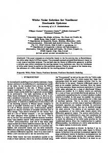
Fig. 1. (a) Typical signal generated by Eq. (19). (b) Steady state PDF P (x) of the signal. The dashed line is the analytical q-exponential expression (20) for the steady state PDF. (c) Power spectral density S(f ) of the same signal. The smooth gray line shows the 1/f slope. The parameters used are λ = 3, η = 2, x0 = 1, and σ = 1.
SDE (19) for x ≥ 0 gives indeed the q-exponential steady state PDF � �λ λ−1 x0 λ−1 P (x) = = expq (−λx/x0 ) , x0 x + x0 x0 q = 1 + 1/λ . (20) The addition of the parameter x0 to the stochastic variable x eliminates the divergence of the power-law distribution of x at x → 0. For small x, x � x0 , Eq. (19) represents the linear additive stochastic process generating the Brownian motion with the steady drift. For large x, ,x � x0 , this equation reduces to the multiplicative SDE (12). This modification of the SDE retains the frequency region with 1/f β behavior of the PSD. Results of the numerical solution of SDE (19) are shown in Fig. 1. We see a good agreement of the numerically obtained steady state PDF (20) with the analytical expression. As is evident from Fig. 1(c), the numerical solution confirms the presence of the frequency region with 1/f PSD. The lower bound of this frequency region depends on the parameter x0 . B. q-Gaussian distribution Another proposed modification of SDE is � � 1 2 dx = σ η − λ (x2 + x20 )η−1 xdt + σ(x2 + x20 )η/2 dW . 2 (21) This nonlinear SDE was introduced in Refs. [33]–[36]. The simple case η = 1 is used in the model of return in Ref. [15]. Eq. (21) allows negative values of the stochastic variable x. The Fokker-Planck equation corresponding to SDE (21) gives q-Gaussian steady state PDF � � � λ2 Γ λ2 x20 � P (x) = √ x20 + x2 πx0 Γ λ−1 2 � � � Γ λ2 x2 � expq −λ 2 , =√ 2x0 πx0 Γ λ−1 2 q = 1 + 2/λ . (22) Introduction of the parameter x0 restricts the divergence of the power-law distribution of x at x → 0. For small |x| � x0 Eq. (21) represents the linear additive stochastic process generating the Brownian motion with the linear relaxation. For large
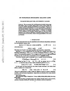
|x| � x0 this equation reduces to the multiplicative SDE (12). This modification of the SDE, even introduction of the negative values of the stochastic variable x, does not destroy the frequency region with 1/f β behavior of the PSD. Results of the numerical solution of SDE (21) are shown in Fig. 2. We see a good agreement of the numerically obtained steady state PDF with the analytical expression (22). As is evident from Figs. 2(c) and (f), numerical solution confirms the presence of the frequency region with 1/f PSD. An interesting particular case of the Eq. (21) is equation dx = σ(x2 + x20 )dW
(23)
corresponding to the parameters η = 2 and λ = 4. This equation does not have a drift term and yields the steady state PDF P (x) ∼ x−4 for large absolute values of |x| � x0 . The complementary cumulative distribution corresponding to P (x) for x � x0 has the form of the inverse cubic law, P> (x) ∼ x−3 . The inverse cubic power-law of the cumulative distributions is one of the stylized facts obtained form the statistical analysis of financial markets. This law is applicable to the developed stock markets, commodity markets and to the most traded currency exchange rates. The exponents that characterize these power laws are similar for different types and sizes of markets, for different market trends and for different countries [37]–[42]. According to Eq. (11), the power spectral density of the signal generated by Eq. (23) has 1/f 1.5 form in a wide region of frequencies. This is confirmed by numerical calculation, shown in Fig. 2(f), as well. IV.
C ONCLUSIONS
Many complex systems exhibit long-range interactions, long-range correlations, multifractality, non-Gaussian distributions with asymptotic power-law behavior. A possible theoretical framework for describing these systems is the nonextensive statistical mechanics that generalizes the Boltzmann-Gibbs theory. An important example of systems featuring q-Gaussian distributions and long-range temporal correlations are financial systems. Proposed equations yielding both the distributions of the nonextensive statistical mechanics and 1/f noise extend understanding of the complex systems and allow to model long-range correlated processes.
(a) x
100
40 30 20 10 0 -10 -20 -30 -40
(b)
10-2
15
20
10
10-4
-1000
(e)
5 x
10-3
10 10 t
-500
0 x
500
100 10-2
10-8 10-10
-10 0
5
10 t
15
20
-1000
100
101
102
103
104
101 100 10-1 10-2 S(f) 10-3 10-4 10-5 10-6 10-7 -1 1000 10
102
103
104
(f)
P(x) 10-6
-5
10-5 -1 10
1000
f
10-4
0
100
S(f) 10-2
-8
5
101
10-1
10-4 P(x) 10-6
0
(d)
(c)
-500
0 x
500
100
101 f
Fig. 2. Typical signal generated by Eqs. (21), (a), and (23), (d); the corresponding steady state PDF P (x) of the signal, (b) and (e), and the power spectral density S(f ), (c) and (f). The parameter λ has the value λ = 3 in (a), (b), and (c) and λ = 4 in (d), (e), and (f). The dashed line in (b) and (e) is the analytical q-Gaussian expression (22) for the steady state PDF. The smooth gray lines in (c) and (f) show the 1/f β slope with β = 1 in (c) and β = 1.5 in (f). Other parameters are η = 2, x0 = 1, and σ = 1.
R EFERENCES [1] [2] [3] [4] [5] [6] [7] [8] [9] [10] [11] [12] [13] [14] [15] [16] [17] [18] [19] [20] [21] [22]
C. Tsallis, Introduction to Nonextensive Statistical Mechanics – Approaching a Complex World. New York: Springer, 2009. ——, Braz. J. Phys., vol. 39, p. 337, 2009. L. Telesca, Tectonophysics, vol. 494, p. 155, 2010. C. M. Gell-Mann and C. Tsallis, Nonextensive Entropy— Interdisciplinary Applications. NY: Oxford Univ. Press, 2004. S. Abe, Astrophys. Space Sci., vol. 305, p. 241, 2006. S. Picoli, R. S. Mendes, L. C. Malacarne, and R. P. B. Santos, Braz. J. Phys., vol. 39, p. 468, 2009. C. Tsallis, J. Stat. Phys., vol. 52, p. 479, 1988. C. Tsallis, A. R. Plastino, and R. S. Mendes, Physica A, vol. 261, p. 534, 1998. D. Prato and C. Tsallis, Phys. Rev. E, vol. 60, p. 2398, 1999. C. Tsallis, Braz. J. Phys., vol. 29, p. 1, 1999. L. Borland, Phys. Rev. E, vol. 57, p. 6634, 1998. ——, Phys. Rev. Lett., vol. 89, p. 098701, 2002. C. Anteneodo and C. Tsallis, J. Math. Phys., vol. 72, p. 5194, 2003. B. Coutinho dos Santos and C. Tsallis, Phys. Rev. E, vol. 82, p. 061119, 2010. S. M. D. Queiros, L. G. Moyano, J. de Souza, and C. Tsallis, Eur. Phys. J. B, vol. 55, p. 161, 2007. C. Beck, Phys. Rev. Lett., vol. 87, p. 180601, 2001. L. M. Ward and P. E. Greenwood, “1/f noise,” Scholarpedia, vol. 2, no. 12, p. 1537, 2007. M. B. Weissman, Rev. Mod. Phys., vol. 60, p. 537, 1988. A. L. Barabasi and R. Albert, Science, vol. 286, p. 509, 1999. T. Gisiger, Biol. Rev., vol. 76, p. 161, 2001. G. Szabo and G. Fath, Phys. Rep., vol. 446, p. 97, 2007. C. Castellano, S. Fortunato, and V. Loreto, Rev. Mod. Phys., vol. 81, p. 591, 2009.
[23] [24] [25] [26] [27] [28] [29] [30] [31] [32] [33] [34] [35] [36] [37] [38] [39] [40] [41] [42]
I. E. Eliazar and J. Klafter, Phys. Rev. E, vol. 82, p. 021109, 2010. B. Kaulakys and J. Ruseckas, Phys. Rev. E, vol. 70, p. 020101(R), 2004. B. Kaulakys, J. Ruseckas, V. Gontis, and M. Alaburda, Physica A, vol. 365, p. 217, 2006. B. Kaulakys and M. Alaburda, J. Stat. Mech., vol. 2009, p. P02051, 2009. J. Ruseckas and B. Kaulakys, Phys. Rev. E, vol. 81, p. 031105, 2010. B. Kaulakys and T. Meˇskauskas, Phys. Rev. E, vol. 58, p. 7013, 1998. B. Kaulakys, Microel. Reliab., vol. 40, p. 1787, 2000. B. Kaulakys, V. Gontis, and M. Alaburda, Phys. Rev. E, vol. 71, p. 051105, 2005. H. Risken and T. Frank, The Fokker-Planck Equation: Methods of Solution and Applications. Springer, 1996. C. W. Gardiner, Handbook of Stochastic Methods for Physics, Chemistry and the Natural Sciences. Berlin: Springer-Verlag, 2004. B. Kaulakys, M. Alaburda, and V. Gontis, AIP Conf. Proc., vol. 1129, p. 13, 2009. V. Gontis, B. Kaulakys, and J. Ruseckas, AIP Conf. Proc., vol. 1129, p. 563, 2009. V. Gontis, J. Ruseckas, and A. Kononoviˇcius, Physica A, vol. 389, p. 100, 2010. J. Ruseckas and B. Kaulakys, Phys. Rev. E, vol. 84, p. 051125, 2011. P. Gopikrishnan, M. Meyer, L. A. N. Amaral, and H. E. Stanley, Eur. Phys. J. B, vol. 3, p. 139, 1998. S. Solomon and P. Richmond, Physica A, vol. 299, p. 188, 2001. X. Gabaix, P. Gopikrishnan, V. Plerou, and E. Stanley, Nature (London), vol. 423, p. 267, 2003. R. K. Pan and S. Sinha, Physica A, vol. 387, p. 495, 2008. B. Podobnik, D. Horvatic, A. M. Petersen, and H. E. Stanley, PNAS, vol. 106, p. 22079, 2009. G.-H. Mu and W.-X. Zhou, Phys. Rev. E, vol. 82, p. 066103, 2010.