have been presented such as Waller-Kraft [15] or Paice [8, 7]. ..... IAn . The following measurement formula yields the measurement value for a given.
1 On the Relation between Fuzzy and Quantum Logic Ingo Schmitt, Andreas Nürnberger, Sebastian Lehrack Summary. Fuzzy logic provides us with a means to deal with concepts like vagueness and uncertainty. Quantum logic was developed in the context of quantum mechanics and in contrast to fuzzy logic, it is not based on membership values but on vector subspaces identified by projectors. Interestingly, there are relations between both theories. The interaction of a projector with a normalized vector produces a value which can be directly interpreted as fuzzy membership value. In this contribution we show that under some circumstances the conjunction of projectors directly corresponds to the algebraic product in fuzzy logic while taking in addition the producing projectors into consideration. Thus, quantum logic gives us means to handle the semantics behind the fuzzy algebraic product and algebraic sum.
1.1 Introduction Fuzzy logic is a well-established formalism in computer science being strongly influenced by the work of Zadeh [17, 16]. It provides us with a means to deal with vagueness and uncertainty. Fuzzy logic is based on t-norms and t-conorms for intersection and union, respectively, on membership values of fuzzy sets. Quantum logic was developed in the context of quantum mechanics. In contrast to fuzzy logic, the logic is not based on membership values but on vector subspaces identified by projectors. The lattice of all projectors provides us with a lattice operations interpreted as conjunction and disjunction. Interestingly, there are relations between both theories. The interaction of a projector with a normalized vector produces a value which can be interpreted directly as fuzzy membership value. This paper shows, that under some circumstances the conjunction of projectors directly corresponds to the t-norm algebraic product in fuzzy logic. However, in contrast to fuzzy logic which is defined on fuzzy sets, quantum logic takes the producing projectors into consideration. As result, we are able to overcome the problem of idempotence for the algebraic product. Furthermore, if we restrict projectors to be mutually commuting we obtain a logic obeying the rules of the Boolean algebra. Thus, quantum logic gives us more insights into the semantics behind the fuzzy norms algebraic product and algebraic sum. In the following, we first give in Sect. (1.2) a brief introduction to Fuzzy Logic and then introduce in more detail in Sect. (1.3) the concepts of Quantum
2
Logic. Finally, we discuss in Sect. (1.4) the relation between both theories and conclude our work in Sect. (1.5).
1.2 Conjunction and Disjunction in Fuzzy Logic If humans describe objects, they effectively use linguistic terms like, for instance, small, old, long, fast. However, classical set theory is hardly suited to define sets of objects that satisfy such linguistic terms. Let us, for examples, assume a person being assigned to the set of tall persons. If a second person is only insignificantly smaller, it should also be assigned to this set, and thus it seems reasonable to formulate a rule like “a person who is less than 1mm smaller than a tall person is also tall” to define our set. However, if we repeatedly apply this rule, obviously persons of any size will be assigned to the set of tall persons. Any threshold for the concept tall will be hardly justifiable. On the other hand, it is easy to find persons that are tall and small, respectively. Modelling the typical cases is not the problem, but the penumbra between the concepts can hardly be appropriately modelled with classical sets. The main principle of fuzzy set theory is to generalize the concept of set membership [17]. In classical set theory a characteristic function 1IA : ( Ω → {0, 1} 1, if ω ∈ A 1IA (ω) = 0, otherwise,
(1.1)
defines the memberships of objects ω ∈ Ω to a set A ⊂ Ω. In fuzzy set theory the characteristic function is replaced by a membership function µM : Ω → [0, 1],
(1.2)
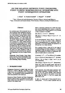
that assigns numbers to objects ω ∈ Ω according to their membership degree to a fuzzy set M . A membership degree of one means that an object fully belongs to the fuzzy set, zero means that it does not belong to the set. Membership degrees between zero and one correspond to partial memberships. Membership degrees can be used to represent different kinds of imperfect knowledge, including similarity, preference, and uncertainty. However, no framework is provided to model the semantics of an element or how the membership values had been derived. Common fuzzy sets are so-called fuzzy numbers (or fuzzy intervals) that assume a value of one for a single value a ∈ IR (or interval [a, b] ⊂ IR), and have monotonously decreasing membership degrees with increasing distance from this core. Fuzzy numbers can be associated with linguistic terms like, for example, “approximately a”. In fuzzy rule based systems, typically parameterized membership functions are used, where these are in most cases either triangular, trapezoidal, or Gaussian shaped (cf. Figure 1.1):
3
Fig. 1.1. Examples of typical fuzzy sets
(x − x0 )2 µx0 ,σ (x) = exp − 2σ 2 �
� .
(1.3)
If the complete input range is covered by overlapping fuzzy sets, this is called fuzzy partition. If their number is sufficiently small, the fuzzy sets M are usually associated with linguistic terms, e.g. AM ∈ {small, medium, large}. Conjunctions and disjunctions of fuzzy membership degrees are evaluated by so-called t-norms and t-conorms, respectively: Definition 1. A t-norm > : [0, 1]2 → [0, 1] is a commutative and associative function that satisfies >(a, 1) = a and a ≤ b ⇒ >(a, c) ≤ >(b, c). Definition 2. A t-conorm ⊥ : [0, 1]2 → [0, 1] is a commutative and associative function that satisfies ⊥(a, 0) = a and a ≤ b ⇒ ⊥(a, c) ≤ ⊥(b, c). For a, b ∈ {0, 1}, all t-norms (t-conorms) behave like the traditional conjunction (disjunction). For the values in between, however, different behaviors are possible. [17] suggest the usage of max for union, min for intersection and 1 − µ(x) for the complement. While there are more functions available [7, 19], every intersection operator has to be a t-norm. First, we will consider min/max the standard because it is the only idempotent and first proposed set of functions [17]. [8] shows that the application of min/max differs from the intuitional understanding of a combination of values (see below). Furthermore, the binary min/max functions return only one value. This leads to a value dominance of one of the two input values while the other one is completely ignored [12, 6, 8]. Thus, min/max cannot express influences or grades of importance of both values on a result, e.g. max(0.01, 1) gives the same result as max(0.9, 1) although the values of the second pair do not differ very much from a human point of view. The form of the complement shows that the fuzzy set theory and its logic does not form a Boolean algebra because the conjunction of x with its complement is not equal 0: x ∧ ¬x = min(x, 1 − x) 6= 0 e.g. for x = 0.5 To overcome the problem of value dominance, parameterized functions have been presented such as Waller-Kraft [15] or Paice [8, 7]. Their parameter
4
basically regulates the behavior of the function between the extrema of a t-norm or t-conorm resulting in a more comprehensible behavior for a human. Alternatively, another pair of norms has been proposed: the algebraic product a · b for intersection and the algebraic sum a + b − a · b for union [7]. They provide means to express statements that involve both values and therefore attenuate the dominance problem of min/max. In contrast to min/max the algebraic product is not idempotent and thus no distributivity holds. This can be easily shown: x ∧ x = x2 6= x. If it is not possible to define exact membership degrees it is sometimes useful to consider only the qualitative order of items. Thus we can define the concept of an L-Fuzzy-Set using the lattice concept: Definition 3. Let (L, u, t) be a lattice with lmin being the smallest element and lmax being the biggest element. Then a L-Fuzzy-Set η of X is a mapping from the base set X to the set L, i.e. η : X → L. L(X) represents the set of all L-Fuzzy-Sets of X.
1.3 Conjunction and Disjunction in Quantum Logic The development of quantum mechanics dates back to the beginning of the last century. The early theoretical foundations were strongly influenced by physicists such as Einstein, Planck, Bohr, Schrödinger and Heisenberg. Quantum mechanics deals with specific phenomena of elementary particles such as uncertainty of measurements in closed microscopic physical systems and entangled states. In recent years, quantum mechanics became an interesting topic for computer scientists who try to exploit its power to solve computationally hard problems. Introductions to quantum logic for non-physicists can be found, e.g., in [5, 2, 11]. 1.3.1 Mathematical and Physical Foundations This subsection gives a short introduction to the formalism of quantum mechanics and shows its relation to probability theory. After introducing some notational conventions, we briefly present the four postulates of quantum mechanics. Here, we assume the reader being familiar with linear algebra. The formalism of quantum mechanics deals with vectors of a complex separable Hilbert space H. For simplicity we present in the following the realvalue view of the formalism. However, the approach can be defined likewise on complex and real vector space. The Dirac notation [3] provides us an elegant means to formulate basic concepts of quantum mechanics:
5
• A so-called ket vector |xi represents a column vector identified � � � �by x. Let 1 0 two special predefined ket vectors be |0i = and |1i = . 0 1 • The transpose of a ket |xi is a row vector hx| called bra whereas the transpose of a bra is again a ket. Both form together a one-to-one relationship. • The inner product between two kets |xi and |yi returning a scalar equals the scalar product defined as the product of hx| and |yi. It is denoted by a bra(c)ket ’hx|yi’. The norm of a ket vector |xi is defined by || |xi || ≡ p hx|xi. • The outer product between two kets |xi and |yi is the product of |xi and hy| and is denoted by ’|xihy|’. It generates a linear operator expressed by a matrix. P • A projector p = i |iihi| is a symmetric (pt = p) and idempotent (pp = p) linear operator defined over a set of orthonormal vectors |ii. Multiplying a projector with a state vector |ϕi means to project the vector onto the respective vector subspace. Each projector p is bijectively related to a closed subspace via p ↔ vsp (H) := {p|ϕi | |ϕi ∈ H}. Despite a projector p can be constructed from P an arbitrary orthonormal basis |ii for vsp (H), the derived projector i |iihi| will be always the identity operator of vsp (H). We can conclude this from the following completeness relation for orthonormal vectors. Let |ii be a vector of an orthonormal basis for vspP (H). Then an arbitrary vector |ψi ∈ vsp (H) can be expressed as |ψi = i vi |ii in vsp (H) for some set of scalars vi . Note that hi|vi = vi and therefore ! X X X p|ψi = |iihi| |ψi = |iihi|ψi = vi |ii = |ψi i
i
i
Since the last equation is true for all |ψi it follows that p is the identity operator for vsp (H). • The tensor product between two kets |xi and |yi is denoted by |xi ⊗ |yi or short by |xyi. If |xi is m-dimensional and |yi n-dimensional then |xyi is an m·n-dimensional ket vector. The tensor product of two-dimensional kets |xi and |yi is defined by: x1 y1 � � � � x1 y2 x1 y1 |xyi ≡ |xi ⊗ |yi ≡ ⊗ ≡ x2 y1 . x2 y2 x2 y2 The tensor product between two matrices A and B is analogously defined: x1 y1 x1 y2 x2 y1 x2 y2 � � � � x1 y3 x1 y4 x2 y3 x2 y4 x1 x2 y1 y 2 AB ≡ A ⊗ B ≡ ⊗ ≡ x3 y1 x3 y2 x4 y1 x4 y2 . x3 x4 y3 y 4 x3 y3 x3 y4 x4 y3 x4 y4 Next, we sketch the famous four postulates of quantum mechanics:
6
Postulate 1: Every closed physical microscopic system corresponds to a separable complex Hilbert space1 and every state of the system is completely described by a normalized (the norm equals one) ket vector |ϕi of that space. Postulate 2: Every evolution of a state |ϕi can be represented by the product of |ϕi and an orthonormal2 operator O. The new state |ϕ0 i is given by |ϕ0 i = O|ϕi. It can be easily shown that an orthonormal operator cannot change the norm of a state: || O|ϕi || = || |ϕi || = 1. Postulate 3: A central concept in quantum mechanics is the nondeterministic measurement of a state which means to compute the probabilities of different outcomes. If a certain outcome is measured then the system is automatically changed to that state. Here, we focus on a simplified measurement given by projectors (each one represents one possible outcome). The probability of an outcome corresponding to a projector p and a given state |ϕi is defined by ! X X hϕ|p|ϕi = hϕ| |iihi| |ϕi = hϕ|iihi|ϕi i
i
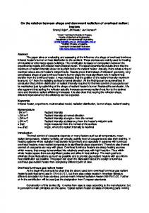
Thus, the probability value equals the squared length of the state vector |ϕi after its projection onto the subspace spanned by the vectors |ii. Due to normalization, the probability value, furthermore, equals geometrically the squared cosine of the minimal angle between |ϕi and the subspace represented by p. Figure 1.2 illustrates the connection between quantum mechanics and probability theory for the two-dimensional case. Please notice that the base vectors |0i and |1i are orthonormal. The measurement of the state |ϕi = a|0i + b|1i with || |ϕi || = 1 by applying the projector |0ih0| provides the squared portion of |ϕi on the base vector |0i which equals a2 . Analogously, the projector |1ih1| provides b2 . Due to Pythagoras and the normalization of |ϕi both values sum up to one. In quantum mechanics where |0ih0| and |1ih1| represent two independent outcomes of a measurement the values a2 and b2 give the probabilities of the respective outcomes. 1 2
For simplicity, we restrict ourselves to the vector space Rn . An operator O is orthonormal if and only if Ot O = OOt = I holds where the symbol ’t ’ denotes the transpose of a matrix and ’I’ denotes the identity matrix.
7 hϕ|0ih0|ϕi = a2 |1i 1
hϕ|1ih1|ϕi = b2 a2 + b2 = 1 a
|ϕi
b
1
|0i
Fig. 1.2. Pythagoras and probabilities
Postulate 4: This postulate defines how to assemble various quantum systems to one system. The base vectors of the composed system are constructed by applying the tensor product ’⊗’ to the subsystem base vectors.
1.3.2 Lattice of Projectors Following [18], we develop here the main concepts of quantum logic originally developed by von Neumann [14]. Applying quantum logic on projectors will give us the capability to measure state vectors on complex conditions. The starting point is the set P of all projectors of a vector space H of dimensions greater than two. We want to remind that each projector p ∈ P is bijectively related to a closed subspace via p ↔ vsp (H) := {p|ϕi | |ϕi ∈ H}. The subset relation on the corresponding subspaces forms a complete partially ordered set (poset) of the projector set P whereby p1 ≤ p2 ⇔ vsp1 (H) ⊆ vsp2 (H). Thus, we obtain a lattice3 with the binary operations meet (u) and join (t) being defined as p1 u p2 := p ↔ vsp (H) := vsp1 (H) ∩ vsp2 (H) p1 t p2 := p ↔ vsp (H) := closure(vsp1 (H) ∪ vsp2 (H)) whereby the closure operation generates here the set of all possible vector linear combinations. Furthermore, the orthocomplement (¬) is defined as ¬p1 := p ↔ vsp (H) := {|ϕi ∈ H | ∀|ψi ∈ vsp1 (H) : hψ|ϕi = 0}. In quantum logic the orthocomplement can be interpreted as negation operator. 3
The laws of commutativity, associativity, and absorption are fulfilled.
8
1.3.3 Boolean Sublattice Quantum logic in general does not constitute a Boolean algebra since the distribution law is violated. To confirm this statement, we consider three projectors p1 , p2 and p3 in a two-dimensional vector space H. The projectors are specified as p1 = |0ih0|, p2 = |1ih1|, and p3 = |vihv| whereby |vi = √ (|0i + |1i)/ 2. We can observe that the closure of (vsp1 (H) ∪ vsp2 (H)) spans the whole vector space H. Contrarily, the intersections (vsp3 (H) ∩ vsp1 (H)) and (vsp3 (H) ∩ vsp2 (H)) collapse to the null vector expressed here by the projector p0 . Thus, we obtain p3 u (p1 t p2 ) = p3 6= p0 = p0 t p0 = (p3 u p1 ) t (p3 u p2 ) violating the distribution law. Fortunately, there exist sublattices of projectors which set up a Boolean algebra. To identify these convenient sublattices we have to take the commutativity of projectors into account. Definition 4 (commuting projectors). Two projectors p1 and p2 of a vector space H are called commuting projectors if and only if p1 p2 = p2 p1 holds. P From i |iihi| and P linear algebra we know that two projectors p1 = p2 = j |jihj| commute if and only if their ket vectors |ii and |ji are vectors of the same orthonormal basis B = {|k1 i, . . . , |kn i} for the underlying ndimensional vector space [2]. In that case, we can define Bp1 and Bp2 , whereby Bp1 ⊆ B andPBp2 ⊆ B, as sets of orthonormal vectors which form the proP jectors p1 = i∈Bp |iihi| and p2 = j∈Bp |jihj|. If two projectors commute 1 2 then their join corresponds to the union of the respective sets of underlying base vectors and their meet to the intersection. Thus, we can redefine the meet, join and orthocomplement operation for commuting projectors. Corollary 1 (sublattice operations for commuting projectors). Let p1 and p2 be two commuting projectors. The lattice operations can be adapted to: X (1.4) p1 u p2 := |kihk| k∈Bp1 ∩Bp2
p1 t p2 :=
X
|kihk|
(1.5)
k∈Bp1 ∪Bp2
¬p1 :=
X
|kihk|
(1.6)
k∈B\Bp1
All projectors over one given orthonormal basis form a Boolean algebra. This is affirmed by Stone’s representation theorem for Boolean algebras [13]. It states that every Boolean algebra is isomorphic to a field of sets and its corresponding union and intersection operation. Here, the field of sets is the common orthonormal basis B = {|k1 i, . . . , |kn i} and the respective algebra is given by its power set 2B forming a subset lattice.
9
A sublattice of projectors is shown in Figure 1.3. Each projector is constructed by a subset of the same orthonormal basis which contains three vectors. The bit code refers to the selected basis vectors from the underlying orthonormal basis. The code [110], for example, refers to the vector subspace spanned by the first two basis vectors. p4 t p5 t p 6 [111]
p 4 ≡ p1 t p2 [110]
p5 ≡ p1 t p 3 [101]
p 6 ≡ p2 t p3 [011] join (t) meet (u)
p 1 ≡ p4 u p5 [100]
p2 ≡ p4 u p 6 [010]
p 3 ≡ p5 u p6 [001]
p1 u p2 u p 3 [000] Fig. 1.3. Sublattice of commuting projectors
Actually, quantum logic can be seen as a generalization of a Boolean algebra: The sublattice over every equivalence class comprising commuting projectors constitutes a Boolean algebra. A concise overview of further important results for quantum logic is given in [1, 9, 10]. 1.3.4 Mapping Objects to State Vectors In this subsection we want to briefly explain the main ideas of mapping objects into the vector space formalism of quantum mechanics. Following, we distinguish between single-attribute and multi-attribute objects. We start our considerations with the encoding of a single-attribute object with attribute A into a separated local vector space HA . Later we will merge different single-attribute spaces HAi to a global multi-attribute one represented by H. Here we only exemplarily describe the mapping of an arbitrary non-negative, numerical value a ∈ [0, ∞) to its corresponding state vector |ai. The state vector |ai is located in HA and represents the current value of the attribute A. Please recall that state vectors need to be normalized. Therefore, we cannot directly map a value to a one-dimensional ket vector. Instead we need at least
10
two dimensions. A two-dimensional quantum system in the field of quantum computation is called a qubit (quantum bit). Since every normalized linear combination of two basis vectors |0i = (1, 0)t and |1i = (0, 1)t is a valid qubit state vector we can encode infinitely many values. That is, we take advantage of the superposition principle of quantum mechanics. Please notice that no more than two vectors can be encoded as pairwise independent (orthogonal) state vectors within a one-qubit system. So, for the one-qubit encoding the state vector |ai is embedded in a two-dimensional vector space spanned by |0i and |1i. Definition 5 (mapping numerical values to qubit states). The normalized qubit state vector |ai for a numerical value a ∈ [0, ∞) is defined by � � 1 1 a 7→ |ai = √ . 2 a a +1 Thus, the numerical value is expressed by the normalized ratio between the two basis vectors |0i and |1i. A more complex object contains more than one attribute value. Therefore, we have to adapt our mapping to a multi-attribute version. A multiattribute object can be regarded as a state vector in a composite quantum system. Adopting Postulate 4, we use the tensor product for constructing multi-attribute state vectors and vector spaces out of single-attribute ones. Definition 6 (multi-attribute objects as tensor products of singleattribute states). Assume, an object o = (a1 , . . . , an ) contains n attribute values and |a1 i, . . . , |an i are their respective state vectors which are embedded in separated Hilbert spaces HA1 ,. . . ,HAn , respectively. Then, the ket vector |oi = |a1 i ⊗ . . . ⊗ |an i = |a1 ..an i represents the object o in a global Hilbert space H = IA1 ⊗ . . . ⊗ IAn whereby IAi is the identity matrix of HAi . 1.3.5 Measurement of Projectors In this subsection we will investigate the measurement of projectors in more detail. In quantum logic projectors are combined to new projectors before any measurement w.r.t. an object takes place. Thus, a projector can be constructed from an arbitrary logical condition formula by applying the meet (u), join (t) and orthocomplement (¬) on projectors. A projector therefore embodies the complete semantics of a well-formed condition. In general, the measurement of a projector p on a given state vector |ai is already introduced (Postulate 3) as ! X X ha|p|ai = ha| |iihi| |ai = ha|iihi|ai. i
i
11
Later we will describe a restriction on the structure of complex conditions which allows us to simplify the measurement of combined projectors significantly. Before we will turn our attention to the measurement of projectors generated by complex conditions, we investigate the single-attribute case. Constructing and Measurement of Single-Attribute Projectors The generation of a certain single-attribute projector corresponds to the encoding of the respective attribute. For instance, we explore here an object o with a numerical attribute A (Def. 5) and a projector pc determined by the numerical condition ’A = c’. Thus, the projector pc is given by pc = |cihc|. It is related to an one-dimensional subspace in the single-qubit system HA . Computing the degree of matching between state vector |oi=|ai and the projector pc = |cihc| yields (1 + ac)2 (a2 + 1)(c2 + 1) � � � � 1 1 whereby |ai = √a12 +1 and |ci = √c12 +1 . The resulting expression is a c equivalent to the squared cosine of the enclosed angle between |ai and |ci. There are different encoding techniques for further attribute domains which influence the construction of projectors [12]. In every case we have to preserve the Boolean character of our algebra which is based on commuting projectors. In particular, it must be guaranteed that only orthogonal conditions per attribute are used. Otherwise, the commutativity of the involved projectors would be violated. For example, it is not possible to support different conditions on the same numerical attribute A. To exemplify that case we assume two conditions ’A = c1 ’ and ’A = c2 ’ generating two one-dimensional projectors in HA . In general, these projectors would not be orthogonal and therefore not commuting. That is, their projectors cannot be based on one common set of orthonormal basis vectors. In consequence of this fact, there is no proper way to express the condition ’A = c1 ∨ A = c2 ’ in a single-qubit system HA . But there also exists a special case for a measurement in which this effect does not occur. Assume, we are only interested in a Boolean result (true ≡ 1 or f alse ≡ 0) for a measurement on a condition ’B = c’. The type of attribute B is called Boolean condition attribute and the constant c is given by a value of the attribute domain DB . Before we present the measurement of a state vector |bi on condition ’B = c’ we have to briefly clarify the mapping of |bi into its corresponding Hilbert space HB . The main idea is to bijectively assign each possible attribute value dB ∈ DB to exactly one basis vector for HB . Thus, a value of DB with |DB | = n is expressed by a vector of a predefined basis of HB = Rn . So, the vector space HB is spanned by the predefined set of n orthonormal basis vectors |dB i where each |dB i corresponds bijectively ho|pc |oi = ha|pc |ai = ha|cihc|ai =
12
to a value dB ∈ DB . Let now C ⊆ DB contain the required values of a condition P over the attribute B. Such a condition is expressed by the projector pC = c∈C |cihc|. Since all possible projectors pC on the domain DB are based on the same basis they commute to each other. In consequence, the introduced adapted meet, join and orthocomplement operation can be applied and those projectors altogether constitute a Boolean algebra. The following theorem shows that quantum measurement (Postulate 3) for conditions on these special attributes yields either 1 or 0 as result. Theorem 1 (measuring Boolean condition attributes). Let B be a Boolean condition attribute and |bi an object state vector in HB . The measurement result of a projector pC (C ⊆ DB ) is given by � 1:b∈C hb|pC |bi = 0 : otherwise. Proof. ! hb|pC |bi = hb|
X c∈C
|cihc| |bi =
X
hb|cihc|bi
c∈C
Due to orthonormality of the basis vectors |ci we can write hb|ci = δ(b, c) where δ is the Kronecker delta. That is, the measurement yields the value 1 only if b ∈ C holds. Otherwise, we obtain the value 0. u t Next we shift to a projector over a single-attribute Ai applying to a multiattribute object |oi = |a1 . . . an i. A condition ’Ai = c’ on a multi-attribute object must be prepared accordingly to the definition of a multi-attribute object (Def. 6). Thus, a single-attribute projector |cihc| needs to be combined with all orthonormal basis vectors (expressed by the identity matrix IAj ) of the non-restricted attributes. Definition 7 (applying single-attribute projectors to multi-attribute objects). Assume, ’Ai = c’ is a condition on attribute Ai . Its projector pc expressing the condition against an n-attribute object is given by pc = IA1 ⊗ . . . ⊗ IA(i−1) ⊗ |cihc| ⊗ IA(i+1) ⊗ . . . ⊗ IAn . The following measurement formula yields the measurement value for a given object |oi=|a1 ..an i. ha1 ..an |IA1 ⊗ . . . ⊗ IA(i−1) ⊗ |cihc| ⊗ IA(i+1) ⊗ . . . ⊗ IAn |a1 ..an i = ha1 |IA1 |a1 i . . . ha(i−1) |IA(i−1) |a(i−1) ihai |cihc|ai i ∗ ha(i+1) |IA(i+1) |a(i+1) i . . . han |IAn |an i = hai |cihc|ai i. The result equals the measurement of the single-attribute object case. That is, the computation of the measurement becomes very easy since we can completely ignore non-restricted attributes.
13
Constructing and Measurement of Multi-Attribute Projectors A projector over different attributes is based on a complex condition which is constructed by recursively applying conjunction, disjunction and negation on atomic conditions. Here, we want to regard a select-condition ’Ai = c’ with an arbitrary constant c as an atomic condition. For combining two projectors conjunctively (∧) we apply the meet operator returning a new projector. Analogously, disjunction (∨) corresponds to the join operator and the negation (¬) of a condition is related to the orthocomplement of a projector. Despite dealing with probability values, quantum logic behaves like Boolean algebra if involved projectors do commute. We assume for the rest of this work a sublattice of commuting projectors, respectively a Boolean algebra. To support the measurement of a combined projector we can directly exploit the structure of the underlying condition. We require conditions to be combined with disjoint sets of restricted attributes. That means, no attribute is restricted by more than one operand of a conjunction or disjunction. We will call this kind of conditions non-overlapping w.r.t. to a set of attributes. Based on the requirement of disjoint conditions we develop simple evaluation rules for logical operations (∧, ∨ and ¬) to measure a combined projector. In particular, the measurement of atomic conditions and the application of these evaluation rules are sufficient to compute the measurement of a projector generated by a complex condition. Negation: The following theorem relates the orthocomplement of projectors to the measurement of a negated condition. Theorem 2 (measurement of negated projectors). Assume, a projector pc expressing an arbitrary condition c is given. The measurement of the negated condition by applying p¬c on an object |oi equals the subtraction of the non-negated measurement from 1: ho|p¬c |oi = 1 − ho|pc |oi. Proof. The orthocomplement for projectors can be also expressed as ¬p ≡ I − p encompassing all projectors orthogonal to p. The expression I stands for the identity matrix. Exploiting this formula and a state vector, we obtain ho|p¬c |oi = ho|I − pc |oi = ho|I|oi − ho|pc |oi = 1 − ho|pc |oi. t u The introduced negation for the measurement extends Boolean negation. However, if a measurement returns a probability value between 0 and 1 then the effect may be surprising. For example, assume an attribute A of the three-valued domain {a, b, c} is given. Surprisingly, as shown in Table 1.1, the negated condition ’¬A = b’ does not equal the condition ’A = a ∨ A = c’. Instead, that
14
condition yields the dissimilarity between the attribute value and the value b. Thus, the measurement value of the value a is smaller than 1. This effect is the direct consequence of dealing with values between 0 and 1. query condition A=b ¬(A = b)
object value a b c 0.75 1 0.75 0.25 0 0.25
Table 1.1. Negation values
Conjunction: We will deduce from the following theorem that the measurement of a projector pa∧b generated by conjunctively combined conditions a and b can be evaluated as algebraic product, if we require disjoint sets of restricted attributes. Theorem 3 (measurement of projectors generated by conjunctively combined non-overlapping conditions). Let pa = p1a ⊗ . . . ⊗ pna be a projector on n attributes and k restrictions on the attributes {a1 , .., ak } ⊆ [1, .., n] with � an ai -restriction : i ∈ {a1 , .., ak } i pa = I : otherwise and pb = p1b ⊗. . .⊗pnb be a further projector with l restrictions on the attributes {b1 , .., bl } ⊆ [1, .., n] � a bi -restriction : i ∈ {b1 , .., bl } i pb = I : otherwise and {a1 , .., ak } ∩ {b1 , .., bl } = ∅. Then, computing the measurement of the projector pa∧b = p1a∧b ⊗ . . . ⊗ pna∧b on an object |oi yields ho|pa∧b |oi = ho|pa |oiho|pb |oi. Proof. The meet operation of projectors is defined over the intersection of the corresponding subspaces. Thus, we obtain following derivation
15
pa u pb = (p1a ⊗ . . . ⊗ pna ) u (p1b ⊗ . . . ⊗ pnb ) = (p1a u p1b ) ⊗ . . . ⊗ (pna u pnb ) = p1a∧b ⊗ . . . ⊗ pna∧b whereby p1a∧b ↔ vsp1a∧b (H) = vsp1a (H) ∩ vsp1b (H), ..., pna∧b ↔ vspna∧b (H) = vspna (H) ∩ vspnb (H) Due to the disjointness {a1 , .., ak } ∩ {b1 , .., bl } = ∅ the vector space of every attribute restriction is intersected with H producing identical restrictions. Thus, all restriction are simply taken over and the projector pa∧b is obtained as pa∧b = p1a∧b ⊗ . . . ⊗ pna∧b with an ai -restriction : i ∈ {a1 , .., ak } pia∧b = a bi -restriction : i ∈ {b1 , .., bl } I : otherwise Due to these restrictions and the rule ha1 b1 |a2 b2 i = ha1 |a2 ihb1 |b2 i the measurement of the projector pa∧b on an object |oi can be calculated by ho|pa∧b |oi = ho|p1a∧b ⊗ . . . ⊗ pna∧b |oi = ho|p1a |oi . . . ho|pka |oi ho|p1b |oi . . . ho|plb |oi ho|I 1 |oi . . . ho|I m |oi {z }| {z }| {z } | ho|pa |oi
ho|pb |oi
1
= ho|pa |oiho|pb |oi whereby m = n − (k + l) is the number of unrestricted attributes. Thus, the measured results for conjunctively combined disjoint projectors are simply multiplied. u t This important result can be exemplified by the following measurement of multi-attribute object o. It is formed by two arbitrary numerical attributes A1 and A2 . The state vector |oi = |a1 i ⊗ |a2 i = |a1 a2 i is located in the vector space H = HA1 ⊗ HA2 whereby HA1 and HA2 stand for single-qubit systems. The corresponding condition of interest is given by ’A1 = c1 ∧ A2 = c2 ’. Initially, we can regard the conditions ’A1 = c1 ’ and ’A2 = c2 ’ as atomic conditions integrated in HA1 and HA2 . Then, the conditions are expressed by the two projectors pc1 = |c1 ihc1 | in HA1 and pc2 = |c2 ihc2 | in HA2 . Before we can combine pc1 and pc2 in H, we have to map the both single-attribute projectors to H. We label the extended projectors in H as p0c1 and p0c2 and their respective sets of orthonormal vectors as Bp0c1 and Bp0c2 . For the construction of p0c1 and p0c2 the original vectors |c1 i and |c2 i must be combined with an orthonormal basis of the respective oppositional vector space HAi (Def. 7). So, the vector |c1 i needs to be combined with all vectors
16
of an arbitrary orthonormal basis for HA1 , and an orthonormal basis for HA2 needs to be combined with the vector |c2 i. Here, we choose {|c1 i, |c1 i} for HA1 and {|c2 i, |c2 i} for HA2 , respectively. Please notice that the overline notation denotes the negation of a vector: |ϕi = |¬ϕi. Thus, we obtain
A1 = c1 :
Bp0c = {|c1 c2 i, |c1 c2 i} 1
⇒ p0c1 = |c1 c2 ihc1 c2 | + |c1 c2 ihc1 c2 | A2 = c2 :
Bp0c2 = {|c1 c2 i, |c1 c2 i} ⇒ p0c2 = |c1 c2 ihc1 c2 | + |c1 c2 ihc1 c2 |
The projectors p0c1 and p0c2 are commuting because they are based on the same orthonormal basis {|c1 c2 i, |c1 c2 i, |c1 c2 i, |c1 c2 i} for H. Therefore, we are able to combine the projectors p0c1 and p0c2 by applying the adapted meet Operation (1.4) for commuting projectors: X pc1 ∧c2 = |kihk| = |c1 c2 ihc1 c2 | k∈(Bp0 ∩Bp0 ) c1
c2
The expected result is obtained when we compute the measurement on the state vector |oi = |a1 a2 i. ho|pc1 ∧c2 |oi = ha1 a2 |c1 c2 ihc1 c2 |a1 a2 i = ha1 |c1 iha2 |c2 ihc1 |a1 ihc2 |a2 i = ha1 |c1 i2 ∗ ha2 |c2 i2 = ha1 |pc1 |a1 i ∗ ha2 |pc2 |a2 i The last equation shows the simple multiplication of the single-attribute measurement results for this example. Disjunction: We know that a Boolean algebra respects the de Morgan law [4]. Therefore, we can compute the measurement for the disjunction of non-overlapping conditions over conjunction and negation and obtain ho|pa∨b |oi = 1 − (1 − ho|pa |oi)(1 − ho|pb |oi) = ho|pa |oi + ho|pb |oi − ho|pa∧b |oi. We are now able to define evaluation rules for the measurement of complex non-overlapping conditions on multi-attribute objects.
17
Definition 8 (negation, conjunction and disjunction of non-overlapping conditions). Let c1 and c2 be two commuting conditions which do not contain overlapping atomic conditions. For the evaluation w.r.t. a given object o we define: evalo (¬c1 ) = 1 − evalo (c1 ) evalo (c1 ∧ c2 ) = evalo (c1 ) ∗ evalo (c2 ) evalo (c1 ∨ c2 ) = evalo (c1 ) + evalo (c2 ) − evalo (c1 ∧ c2 )
(1.7) (1.8) (1.9)
To evaluate overlapping conditions we have to apply an evaluation and transformation algorithm which exploits the already introduced rules and the following special case of mutually excluding conditions. Theorem 4 (measurement of projectors generated by disjunctively combined exclusive conditions). Assume, a projector pc1 ∨c2 is determined by the condition c1 ∨ c2 whereby c1 ≡ (u ∧ e1 ) and c2 ≡ (¬u ∧ e2 ) are commuting exclusive subconditions. Moreover, the literals u and ¬u represent two mutually excluding atomic conditions and the subformulas e1 and e2 can be formed by arbitrary conditions. Computing the measurement of the projector pc1 ∨c2 on an object |oi yields ho|pc1 ∨c2 |oi = ho|pc1 |oi + ho|pc2 |oi. Proof. Since the projectors pc1 and pc2 are commuting we can apply the adapted join Operation (1.5) to measure pc1 ∨c2 . Let Bpc1 and Bpc2 the sets of orthonormal basis vectors for pc1 and pc2 . We can state that the intersection of Bpc1 and Bpc2 is always empty because the first component of each basis vector |u . . .i for pc1 is different from the first component of each basis vector |¬u . . .i for pc2 . Thus, we obtain ho|pc1 ∨c2 |oi = ho|
X
|kihk| |oi
k∈Bpc1 ∪Bpc2
=
X
X
ho|kihk|oi +
k∈Bpc1
= ho|
ho|kihk|oi
k∈Bpc2
X
|kihk| |oi + ho|
k∈Bpc1
X
|kihk| |oi
k∈Bpc2
= ho|pc2 |oi + ho|pc2 |oi t u Based on the last theorem we can formulate a further evaluation rule.
18
Definition 9 (disjunction of overlapping exclusive conditions). Let c1 and c2 be two commuting, exclusive and overlapping conditions. We can formulate the following evaluation rule: evalo (c1 ∨ c2 ) = evalo (c1 ) + evalo (c2 ).
(1.10)
Our evaluation algorithm transforms expressions with overlapping conditions into exclusive ones by applying Boolean rules. To compute the measurement of the transformed conditions the rules of Definition 8 and 9 are used. Evaluation algorithm: The algorithm evaluates a given condition w.r.t. a given object. We will show that our evaluation is based on simple boolean transformations and basic arithmetic operations. The algorithm for transforming an condition c is given in Figure 1.4.
input: condition c output: non-overlapping or mutually excluding condition c transform expression c into disjunctive normal form x ˆ1 ∨ . . . ∨ x ˆm where x ˆi are conjunctions of literals (2) simplify expression c by applying idempotence and invertibility4 rules (3) if there is an overlap on a attribute between some conjunctions x ˆi then (3a) let u be a literal of an attribute common to at least two conjunctions (3b) replace all conjunctions x ˆi of c with (u ∧ x ˆi ) ∨ (¬u ∧ x ˆi ) (3c) simplify c by applying idempotence, invertibility, and absorption and obtain c = (u ∧ x ˆ1 ) ∨ . . . ∨ (u ∧ x ˆm1 )∨ (¬u ∧ x ˆm1 +1 ) ∨ . . . ∨ (¬u ∧ x ˆm2 ) (3d) replace c with (u ∧ e1 ) ∨ (¬u ∧ e2 ) where e1 = x ˆ1 ∨ . . . ∨ x ˆm1 , e2 = x ˆm1 +1 ∨ . . . ∨ x ˆm2 (3e) continue with step (3) for e1 and e2 (4) transform innermost disjunctions to conjunctions and negations by applying de-Morgan-law (1)
Fig. 1.4. Transformation algorithm to resolve overlaps
19
Analyzing the transformation result, we observe that the subformulas of the innermost disjunctions (the leaves of the corresponding tree) are mutually non-overlapping on attributes5 before we apply the fourth step. Thus, we can directly apply Formula (1.9). All other disjunctions are based on exclusive subformulas (generated by step (3d)). That is, we can apply Formula (1.10) and simply add the scores. Since, furthermore, all conjunctions are based on non-overlapping subformulas Formula (1.8) directly applies. The fourth step is to simplify arithmetic calculations of multiple disjunctions. Finally, we demonstrate the evaluation algorithm using an object o formed by five attributes. Assume, the condition c is given by c ≡ (A1 = d ∧ ((A2 = e ∧ (A3 = f )) ∨ (A2 = ¬e ∧ A4 = g))) ∨ A5 = h whereby d, . . . , h are numerical constants. Note that A2 = e and A2 = ¬e are orthogonal conditions. Hence, their corresponding projectors are commuting, despite they restrict the same attribute. Consequently, we can still apply the introduced evaluation rules for commuting projectors. In Figure 1.5 we abbreviate atomic conditions and attributes to the labels of the corresponding constants d, . . . , h whereby do stands for the expression evaloA1 (d).
c ≡ (d ∧ ((e ∧ f ) ∨ (¬e ∧ g))) ∨ h (1)(2)
(e ∧ d ∧ f ) ∨ (¬e ∧ d ∧ g) ∨ h (3a)(3b)(3c)
u=e
(e ∧ d ∧ f ) ∨ (e ∧ h) ∨ (¬e ∧ d ∧ g) ∨ (¬e ∧ h) (3d)
(e ∧ ((d ∧ f ) ∨ h)) ∨ (¬e ∧ ((d ∧ g) ∨ h)) (4)
(e ∧ ¬ (¬ (d ∧ f ) ∧ ¬h)) ∨ (¬e ∧ ¬ (¬ (d ∧ g) ∧ ¬h)) arithmetic evaluation w.r.t. data object o: evalo (c) = eo (1 − (1 − do f o ) (1 − ho )) + (1 − eo ) (1 − (1 − do g o ) (1 − ho ))
Fig. 1.5. Example transformations and arithmetic evaluation 4 5
invertibility: a ∨ ¬a = 1, a ∧ ¬a = 0, ¬¬a = a Otherwise the algorithm would not have stopped.
20
Summarising, we can emphasise again that we are now able to evaluate an arbitrary commuting condition by means of the transformation algorithm and simply arithmetic operations.
1.4 Fuzzy Logic versus Quantum Logic After recapitulating fuzzy logic in Section 1.2 and introducing quantum logic we will interrelate and compare concepts from both worlds. Both logics deal with non-Boolean fulfillments of object conditions. Table 1.2 shows correspondences between their underlying concepts. quantum logic normalized vector projector measurement projector complement lattice operations - meet on disjoint projectors - join on disjoint projectors
fuzzy logic object fuzzy set complement of a fuzzy set fuzzy set operations - t-norm algebraic product - t-conorm algebraic sum
Table 1.2. Correspondences between quantum and fuzzy logic concepts
The basic connection between a measurement by a projector p and a fuzzy set s with respect to an object o is given by µs (o) = ho|p|oi. Both logics follow different ways of combining conditions being graphically depicted in Figure 1.6: µs1 ∩s2 (o) = >(µs1 , µs2 ) versus ho| u (p1 , p2 )|oi µs1 ∪s2 (o) = ⊥(µs1 , µs2 ) versus ho| t (p1 , p2 )|oi In fuzzy logic, conjunction and disjunction are directly based on a t-norm (>) and a t-conorm (⊥), respectively, on membership values. In quantum logic, however, these operation are performed on projectors before any evaluation takes place. This fundamental difference gives quantum logic an advantage by allowing it to consider query semantics during combining complex conditions. Thus, we are able to see that the conjunctive combination only of disjoint conditions in quantum logic yields the same result as the algebraic product in fuzzy logic. The test on disjointness, however, is not feasible in fuzzy logic since a t-norm is defined purely on membership values. That property of the quantum approach allows us to differentiate semantical cases during the evaluation. Thus, if we restrict our quantum conditions to commuting projectors then all rules of a boolean algebra are obeyed. This
21 u ho|p|oi ¬
p=
P
i
|iihi|
[0, 1]
t
∩ µs (o)
fuzzy set s
[0, 1]
¬
∪ Fig. 1.6. Construction of complex conditions in quantum and in fuzzy logic and their evaluations
is impossible in fuzzy logic because required semantics (conditions are commuting) is hidden behind the fuzzy sets. From this point of view we conclude, that quantum logic can takes more condition semantics into account than fuzzy logic can do. A bridge between quantum logic and fuzzy logic can be established if we use the generalized definition of a fuzzy set over conditions which is called an L-fuzzy set. The lattice operations meet(∧), join(∨), and complement are then used for conjunction, disjunction and negation on conditions. The lattice is, of course, our projector lattice. This bridge in combination with the algebraic product as t-norm and the algebraic sum as t-conorm is depicted in Figure 1.7 where we assume disjoint conditions. We use the by-pass over the projector lattice in order to prove that the algebraic product provides correct answers. In practice, we can directly apply the algebraic product on object evaluations but only if the underlying conjunctively combined conditions are disjoint.
1.5 Conclusion In our contribution we investigated the relation between concepts from fuzzy logic and quantum logic. For commuting conditions we could show that quantum logic follow the rules of a Boolean algebra. As main difference between fuzzy and quantum logic we identified the way how conditions are combined by conjunction and disjunction with respect to a given object: combination in quantum logic is performed before and in fuzzy logic after object evaluation takes place. Therefore, in quantum logic we are able to test conditions to be combined on disjointness. In case of disjointness the effect of quantum combination coincides with the the fuzzy combination using algebraic product
22 ho|p1 u p2 |oi p1 u p2
[0, 1]
µp1 (o) = ho|p1 |oi
=
µp2 (o) = ho|p2 |oi µp1 ∧p2 (o) = ho|p1 |oiho|p2 |oi [0, 1]
[0, 1]
ho|p1 u p2 |oi = µp1 ∧p2 (o) = µp1 (o) ∗ µp2 (o) = ho|p1 |oiho|p2 |oi Fig. 1.7. CQQL evaluation of conjunctively combined and disjoint conditions on object o
and norm. If disjointness is not fullfilled then an algorithm basing on rules from Boolean algebra is presented which converts any complex condition into a disjoint condition. Besides theoretical insights into the relation between both worlds we learnt we how to use the t-norms algebraic product and sum in order to obtain a Boolean algebra. In future work we will investigate how to deal with non-commuting conditions. Furthermore, we plan to construct a complete database query language in order to integrate concepts from information retrieval into classical database systems.
References
1. E. Beltrametti and B.C. van Fraassen, editors. Current Issues in Quantum Logic. Plenum Press, 1981. 2. I. Chuang, M. A. Nielsen, and I. L. Chuang. Quantum Computation and Quantum Information. Cambridge University Press, 2000. 3. P. Dirac. The Principles of Quantum Mechanics. Oxford University Press, 4th edition, 1958. 4. P. Dwinger. Introduction to Boolean algebras. Physica Verlag, Würzburg, 1971. 5. J. Gruska. Quantum Computing. McGraw-Hill, 1999. 6. Aljoscha Klose and Andreas Nürnberger. On the properties of prototype-based fuzzy classifiers. IEEE Transactions on Systems, Man, and Cybernetics Part B, 37(4):817–835, 2007. 7. Rudolf Kruse, Joerg Gebhardt, and Frank Klawonn. Fuzzy-Systeme. Teubner, Stuttgart, Germany, 1993. 8. Joon Ho Lee, Myoung Ho Kim, and Yoon Joon Lee. Ranking Documents in Thesaurus-based Boolean Retrieval Systems. Inf. Process. Manage., 30(1):79– 91, 1994. 9. P.F. Lock. Connections among quantum logics, part 1: Quantum propositional logics. International Journal of Theoretical Physics, 24:43–53, 1985. 10. P.F. Lock. Connections among quantum logics, part 2: Quantum event logics. International Journal of Theoretical Physics, 24:55–61, 1985. 11. E. Rieffel and W. Polak. An introduction to quantum computing for nonphysicists. ACM Computing Surveys, 32(3):330–335, 2000. 12. Ingo Schmitt. Qql: A db&ir query language. VLDB J., 17(1):39–56, 2008. 13. M. H. Stone. The Theory of Representations of Boolean Algebras. Transactions of the American Mathematical Society, 40:37–111, 1936. 14. J. von Neumann. Grundlagen der Quantenmechanik. Springer Verlag, Berlin, Heidelberg, New York, 1932. 15. W. G. Waller and D. H. Kraft. A mathematical model for a weighted boolean retrieval system. Information Processing and Management, 15(5):235–245, 1979. 16. Lofti A. Zadeh. Fuzzy Logic. IEEE Computer, 21(4):83–93, April 1988. 17. Lotfi A. Zadeh. Fuzzy Sets. Information and Control, (8):338–353, 1965. 18. Martin Ziegler. Quantum Logic: Order Structures in Quantum Mechanics. Technical report, University Paderborn, Germany, 2005. 19. H.-J. Zimmermann. Fuzzy Set Theory -and its applications (3rd ed.). Kluwer Academic Publishers, Norwell, MA, USA, 1996.