Resource Location and Relocation Models with Rolling Horizon Forecasting for Wildland Fire Planning Joseph Y.J. Chow Department of Civil and Environmental Engineering Institute of Transportation Studies 4000 Anteater Instructional Research Building University of California, Irvine Irvine, CA, 92697
[email protected]
Amelia C. Regan Department of Computer Science Institute of Transportation Studies 4068 Donald Bren Hall University of California, Irvine Irvine, CA, 92697
[email protected]
ABSTRACT A location and relocation model are proposed for air tanker initial attack basing in California for regional wildland fires that require multiple air tankers that may be co-located at the same air base. The Burning Index from the National Fire Danger Rating System is modeled as a discrete mean-reverting process and estimated from 2001-2006 data for select weather stations at each of 12 California Department of Forestry’s units being studied. The standard pmedian formulation is changed into a k-server p-median problem to assign multiple servers to a node. Furthermore, this static problem is extended into the time dimension to obtain a chanceconstrained dynamic relocation problem. Both problems are solved using branch and bound in the numerical example. The relocation model is shown to perform better than the static location model by as much as 20-30% when using fire weather data to forecast short term future demand for severe fires, whereas relocating without rolling horizon forecasting can be less cost-effective than a static location model. The results suggest that state fire agencies should identify the threshold beyond which it would be more cost-effective to adopt a regional relocation model with forecasting from fire weather data, especially in a global warming environment.
Key Words Fire resource location, rolling horizon, relocation, constraint programming, stochastic process, mean reversion Accepted for publication in INFOR: Information Systems and Operational Research
1
1. BACKGROUND Recent fires in Southern California have dealt a devastating blow to the environment, to wildlife, to housing stocks and human life. The recent Los Angeles “station fire” of 2009 was one of the worst in history. In 2007 for example, the fires in San Diego County “claimed ten lives, destroyed more than 1,700 homes, burned more than 300 square miles and forced the evacuation of an estimated 500,000 people” (USA Today, Feb 19, 2008). A recent Los Angeles Times article (Boxol, December 31, 2008) estimates that the cost of combating wildland fires in California now exceeds $1 billion. This type of headline is becoming ever-more prominent, and the fire situation is likely to worsen in the future. In Rapp’s (2004) study, nation-wide climate trends were modeled using annual data from 1895 to the present day and forecasted for the next 100 years. Results indicate that the southwestern United States will have wetter winters and warmer summers, leading to more woodland growth in the forests and more grass in the desert regions. This, in turn, will increase the risk of fire outbreaks. Efficient fire and forestry management will only become more crucial over time. In California, this role is handled by the Department of Forestry and Fire Protection (CDF), which is divided into 21 units under its control (each unit generally comprises more than one county) and 6 counties in which fire protection is handled under individual private contracts. Fire protection plans developed by the agency involve stakeholder contributions, priorities, strategic areas for pre-fire planning and fuel treatment plans for local regions. “Hotshot crews” are recruited during the fire season to deal with extreme situations involving large-scale fires. These crews are required to be on-call 24 hours a day, 7 days a week, and must be available within two hours of a call (CDF, 2008). When the Santa Ana winds in Southern California caused a second major fire outbreak in Malibu in 2007, hundreds of firefighters and equipment from throughout the state were available to deploy to the region for a week in response to predictions about the winds (KNBC, 2007). On the other hand, fire authorities had insufficient resources during the first outbreak several weeks prior, and needed to request last minute aid from neighboring regions. There is currently no systematic operational level model for using daily fire weather data to optimally redeploy resources. Our research seeks to remedy this situation. Four goals are achieved in this research. First, fire weather data are modeled as independent mean reverting processes, and results are shown for the estimation of the parameters for each of the CDF units in California for which data was available. Second, a new static resource allocation model that relies on seasonal average fire weather data is developed. Third a chance-constrained dynamic fire resource allocation model that relies on independent observations of fire weather data as first order Markov processes is developed. Note that here we mean dynamic in the sense that the relocation model depends on the previous time-state and the updated fire weather data. The dynamic model differs from the static one in that it can incorporate rolling horizon forecasts of future fire conditions which are based on the mean reverting processes mentioned above. Finally, we compare the performance of these two new models against actual allocations using data from July through August 2006 and 2007. Our analysis shows that the dynamic resource relocation model using rolling horizon forecasts of future conditions can obtain more cost effective results than the methods currently applied as well as both the static location model and the dynamic relocation model with no forecasts. Explicitly incorporating forecasts of short term future demand in the relocation
2
program can incorporate the value of flexibility in the positions of the resources so that excess relocations can be avoided. 2. LITERATURE REVIEW 2.1. Fire Weather Data Fire weather data are important inputs into the decision-making processes of fire management authorities. For example, in Australia, the Bureau of Meteorology provides fire weather data as part of a national framework for fire protection. The senior meteorologists provide two sets of day to day operational outputs for each region, a public set as well as more private, detailed information for decision support to fire authorities (Gunasekera et al, 2006). In Canada an historical Large Fire Database has been developed which includes information on fire location, start date, final size, cause and suppression action for all fires larger than 200 hectares (2 km2 ~ 500 acres) in area for Canada for the 1959-1999 period (Stocks et al, 2003, Amiro et al, 2004). Until the last few decades, fire authorities relied only on simple tools such as relative humidity or maximum daily temperature to describe fire weather. In the last few years, multiple models and indices were developed to suit the needs of local forecasters and fire authorities. Today, different land management agencies across the U.S. in both the public and private sector utilize fire indices which rely on some form of atmospheric input. Several popular indices include the Canadian Fire Weather Index (CFWI), the Keech-Byram Drought Index (KBDI), the Haines Index (HI), the Fosberg Fire Weather Index (FFWI), and the Davis Stability Index. Until the last few years, however, only the HI was tested and scientifically validated by the peer-review process (Potter et al, 2003). The HI produces an integer between 2 and 6 with higher values indicating dry, unstable atmosphere conducive to large wildfires, and is used as an indicator that small fires could become large and erratic. The HI is currently accepted by many fire weather forecasters and fire managers as a useful tool for evaluating atmospheric conditions in fire fighting on any given day. It was shown that HI works well for plume-dominated fires, but not so much for wind-driven fires such as the Santa Ana winds in California (Potter and Martin, 2001). Several studies done in the past for the state of California have relied on other indices based on the National Fire Danger Rating System (NFDRS), such as Gruelich and O’Regan (1982) and Haight and Fried (2007). Among the indices included in the NFDRS are the Energy Release Component (ERC) and the Burning Index (BI). The BI is an index used to relate the potential amount of effort needed to contain a single fire. The BI can be used as a guideline for staffing levels (ratings from 1 for lowest demand to 5 for the highest) (NFDRS, 2008). 2.2. Facility Location Problems Facility location problems represent a rich and broad field with many different subproblems applicable to a multitude of industries, both private and public. Among the literature reviews available, Owen and Daskin (1998), Drezner (2002, especially the chapter by Marianov and Serra) and Snyder (2006) each provide a very broad summary of the development of this field of problems, including dynamic models, public sector models, stochastic models, and scenario planning models. Brotcorne et al (2003) review ambulance location models specifically, comparing application success stories such as Church and ReVelle’s (1974) Maximal Cover Location Problem (MCLP) implemented in Austin, Texas, as well as Daskin’s
3
(1983) Maximal Expected Covering Location Problem (MEXCLP) implemented in Bangkok in 1987. In both cases, cost savings and average response times improved. Another excellent paper discussing emergency vehicle deployment is Goldberg (2004). Haghani and Yang (2007) present an extensive literature review related to real-time emergency vehicle location and propose their own model which incorporates a spatial rolling horizon framework for an urban setting. Berman and Odoni (1982) formulated a dynamic p-median relocation problem that responds to changes in the state of the network. The objective is to minimize steady-state expected service time and cost of relocations taking into account all the potential future allocation states. However, that formulation can quickly become intractable when a large number of facilities are involved. Berman and LeBlanc (1984) expanded on the dynamic model by making the travel times stochastic, and treating peak and off-peak periods as separate states. As the relocation cost increases due to changing states and travel times, the location/relocation strategy changes. With increasing relocation costs, the optimal strategy will involve less relocations. Facility location problems have been used to address fire emergencies for several decades. According to Badri et al (1998), insurance service offices use the distance between customers and fire companies to rate the fire protection capabilities in different cities. Kolesar and Walker (1974) developed a computationally efficient heuristic algorithm to relocate firefighters based on calls received in districts within New York City. Their algorithm included an inconvenience cost associated with the relocations, and provided rules for constraints, such as considering relocations only for fires lasting longer than half an hour. Other urban fire covering models have been developed in the last few years as well (for example Haghani and Yang, 2007). However, an urban fire location model differs significantly from one applicable to wildland fires, where simultaneously occurring fires are less likely but a single fire may require multiple fire resources. A wildland fire location model should require the k closest facilities to cover a demand node. Marianov and Serra (2002) show that the p-median problem (PMP) can be modified by adding a constraint for a minimum demand threshold level to require a minimum number of servers to cover each node. Co-location is locating multiple servers at a node, and it is another important feature to consider in wildland fire and other large-scale disaster resource models. Marianov and Revelle (1991) develop a facility co-location covering problem in which multiple response vehicles can be deployed to a single location. However, the purpose of co-location in the urban application is to deal with probabilities that the servers would be busy with another event. Their formulation indicates whether the kth server is located at site j using a binary variable for each server. 2.3. Wildland Fire Resource Location and Deployment Models According to Martell et al (1998), there remain many important challenges for fire deployment such as having regional fire duty officers decide each day how many fire fighters and transport vehicles should be deployed at initial attack bases. There is such a need because the 2-5% of fires that escape initial attack can cause a disproportionate amount of damage (MacLellan and Martell, 1996). The problems in regional wildland fire resource location and deployment such as air tanker initial attack planning is that one air tanker may not be enough to cover a potential fire, and there is typically more than one air tanker co-located at an airbase.
4
Static location models have been developed using MCLP to locate wildland fire resources. Dimopoulou and Giannikos (2001) conducted such a study using an MCLP formulation. Haight and Fried (2007) is a recent example of using a variant MCLP formulation with scenario planning to address uncertainty. They propose a multi objective covering model to deploy fire engines to stations that require a certain number of resources on a particular day. The model relies on the output of a fire occurrence simulator to determine the probability that a fire occurs at a node and also the distribution associated with the number of resources needed to contain the fire. Their formulation allows multiple resources to cover a node with co-location considered. The trade-off between using a MCLP versus a PMP is that the PMP has an order of magnitude more decision variables but considers a more detailed objective value (in our case it’s the travel time of air tankers instead of the sum of binary coverage variables). For example, if there are two nodes A and B that are within coverage distance and node A has demand requirement of 3 air tankers versus 1 from node B, an MCLP cannot differentiate between a solution of placing 4 air tankers on A or B (both cover the nodes). On the other hand, the PMP would prefer a solution with 3 air tankers on A and 1 air tanker on B because they have shorter deployment times. This differentiation is especially important in comparing the performance between a static model and a dynamic relocation model. State-dependent probabilistic models, such as those shown in Gruelich and O’Regan (1982) and MacLellan and Martell (1996), consider the deployment of resources given transition probabilities from one state to another. While this approach allows multiple resources to be assigned to a demand node, it does not share the resources across nodes the way a facility location model would. Several papers assume or acknowledge that fire weather data can be modeled as a first order Markov process (Gruelich and O’Regan, 1982, MacLellan and Martell, 1996), and Martell (1999) proves this is the case for the Fire Weather Index in Ontario. Martell concludes that if Markov models can be used to model day to day changes in fire danger rating indices, the properties of Markov chains can be exploited to improve fire management planning. 3. PROBLEM STATEMENT To be clear, we examine the problem of allocating air tankers to air bases over the course of a wildfire season so as to minimize the cost and time of deploying such air tankers to actual fires. While the numerical examples and problem are defined for air tanker basing, it can also be generalized for any resource location and relocation modeling for regional networks with demand nodes that may require multiple servers to cover. 4. MODEL FORMULATIONS 4.1. Demand Let the state of the network be defined by the demand levels at each node at a discrete point in time (a single day), where these demand levels (resource allocations based on fire weather, not on actual fire occurrences) are stochastic on a day-to-day basis for a particular season, such as July through August each year. Since the fire weather indices can be assumed to be first order Markov processes, the BI at each node is modeled as a discretized mean-reverting Ornstein-Uhlenbeck (O-U) process.
5
Although O-U is a continuous process, it can be shown that a discrete AR(1) process can converge weakly to the O-U process (Tanaka, 1996). Note that we start with this model rather than using the AR(1) process directly to allow for the possibility of the availability of richer continuous data in the future. If the BI follows a discrete mean-reverting O-U process, then it can be represented by equation (1) below using three parameters: mean reversion rate αj, mean µj, and volatility σj. dqtj = α j ( µ j − qtj )dt + σ j dWt (1) Where j is the demand node, t is a time-state, dWt is an increment in the Wiener process (also known as Brownian motion) which is assumed to be i.i.d. N(0, t), and qtj is the fire weather index value at time t for node j. The BIs for all nodes are assumed to be independent of each other, although in reality there should be some relationship between the BI and actual fire occurrences for adjacent nodes depending on the distance and geography separating the nodes. For a large regional model like the state of California however, this interdependency can reasonably be relaxed. The parameters of equation (1) can be calibrated using the least squares regression method described in Van den Berg (2008) for each demand node based on historical data. Although static location models do not need to make use of this characterization of fire weather indices since they can rely on seasonal averages, the proposed dynamic relocation model can incorporate this information in its chance constraint formulation to introduce anticipation into the model. We start with a static location model and then proceed to modify that model into the proposed relocation model. 4.2. Static k-server p-Median Problem (KPMP) Let a network be defined as G(N,A) of N nodes and A arcs with fixed travel times and demand for fire protection be linearly dependent upon the Burning Index (BI) value. Let there be a fixed number of fire resources, P. The objective is to use a PMP model that includes the minimum demand thresholds discussed by Marianov and Serra (2002) while also including co-location. Instead of enumerating each kth server with a binary variable, we will use integers to represent the number of servers located at a node. We call this model formulation the k-server p-Median Problem (KPMP), where p servers are located such that the ki closest servers are assigned to each demand node i and where co-location is possible. Min
∑∑ d
Z ij
(2a)
Z ij − X j ≤ 0, ∀i, j
(2b)
∑Z
(2c)
i
s.t.
ij
j
ij
≥ ki
∀i
j
∑X
j
=P
(2d)
j
X j ≥ 0 ∀j , Z ij ≥ 0 ∀i, j , Zi, Xj integers
(2e)
Where Zij = integer number of servers (air tankers) at node j covering node i dij = matrix of distances from i to j
6
Xj = integer number of servers (air tankers) based at node j ki = minimum demand threshold for number of servers (air tankers) covering node i P = the number of servers (air tankers) in the network
In this model, the demands at each node are shifted into the constraints and the decision variables are changed from binary variables to integer variables. (2a) minimizes the distances of the closest servers in terms of deployment time. The objective will naturally force all the Zij’s to be zero unless they are the k closest servers. (2b) guarantees that for a given base node, the number of servers assigned to cover any individual demand node does not exceed the number of servers available at that base node. (2c) forces the k closest servers to a node i to be chosen, whether they are at the same node j or at different nodes. (2d) and (2e) are the facility budget constraint and non-negativity constraints. We assume that the Burning Index (BI) is reasonably represented by the linear equation shown in (3): k i = δqi (3) Where qi is the average value of the BI over a given time period (in our case a two month season), and δ is a scaling parameter to convert the average BI to average air tanker staffing needs. For the static model the seasonal mean value of the BI’s are used. Since the staffing levels are unknown or may vary depending on location, a reasonable value of δ is chosen that is high enough to differentiate changes in the BI values but low enough to avoid hitting the maximum P facilities ceiling. In addition, the relationship between BI and air tankers needs is assumed to be linear. This is backed up by the National Fire Danger Rating System provided by the National Oceanic and Atmospheric Administration (NFDRS, 2008). Naturally, if this function were better understood then additional relevant information could easily be incorporated into our model. The calibration of δ is important for actual implementation, but for comparison between different model performances, a reasonable value should suffice. Note that a promising topic of future research would be to examine alternative methods for modeling and calibrating this demand constant δ. There are N(N+1) integer decision variables and 2N2+2N+1 constraints in this problem. As this is a more complex version of the p-median problem, it is also NP-Complete. A branch and bound approach can be used for the simplified California network shown in the example, but for more complex problems with many additional decision variables a heuristic will be necessary.
4.3. Chance-constrained Dynamic k-server Relocation Problem (CDKRP) Instead of a static, seasonal location model, consider a day-to-day model where the resource basing relocation decisions need to be made. The demand in the static model, ki, is now a function of a stochastic variable ݍ௧ representing a fire weather index that changes day-to-day. A chance-constrained dynamic relocation formulation of the KPMP is developed to minimize the deployment time for each time-state and to consider relocation if the benefit of a relocation is greater than the cost of transportation. The relocation is determined from anticipating the expected deployment times over a forecasted rolling time horizon T (e.g. 7-day forecast) based on the current day’s fire weather data. In other words, if the fire weather station at some node updates its BI value to a significantly high value, it is more likely to be high in the next T days depending on its characterized mean-reversion process. The idea of optimizing the locations based on multiple time periods is similar to one proposed by Repede and Bernardo (1994). Their model, referred to as the TIMEXCLP approach,
7
considers an expected covering problem for multiple time periods. The CDKRP uses a p-median problem where the future demand is obtained from the expected value of the demand using the mean-reverting process. To be clear, here we develop a relocation model that considers the impact of the decision for multiple time states (days). That said, we make the simplifying assumption (through the use of a chance constraint) that the impact of the decision depends only on the new relocation and current relocation, not on subsequent relocations on future time periods because that would make the model too complex. Such a model would require dynamic programming to solve and would be intractable for problems of realistic size (as shown in Berman and Odoni, 1982). Instead, we show that with this simplifying assumption we can still make significant improvement to the performance of the system. To explain how this rolling horizon model works let’s select an arbitrary day, say day 10. If on day 10 we run this model, it will tell us whether we should relocate, given day 9’s locations and day 10’s fire weather update. We would use the mean-reverting process to predict the demand for the next few days (days 11, 12, 13) to determine the impact of the service time (via chance constraint) for the current location for all 4 days (10 – 13) – but not to determine relocation on all 4 days because that would be too complex. After relocation decisions are made on day 10, the next day approaches (day 11) and fire weather data is updated. On that day, we would forecast days 12, 13, 14, and determine whether it is worth relocating on day 11 only. We propose the following model, which we call a Chance-constrained Dynamic k-server Relocation Problem (CDKRP): t +T
Φ t = min ∑∑∑ d ij Z ijτ + λ ∑∑ crsYrs X
τ =t
i
j
r
(4a)
s
s.t.
Z ijτ − X tj ≤ 0, ∀i, j,τ ∈ [t , t + T ]
∑ Z τ ≥ min(P, E [k τ ]+ 1.645δσ ij
j
j
τ −t
)
(4b)
∀ i,τ ∈ [t , t + T ]
(4c)
j
∑X
t j
=P
(4d)
j
− S r − X rt −1 + X rt ≤ 0, ∀r
(4e)
− Ds + X st −1 − X st ≤ 0, ∀s
(4f)
∑Y
= S r , ∀r
(4g)
∑Y
= Ds , ∀s
(4h)
rs
s
rs
r
X tj ≥ 0 ∀j , t , Z ijτ ≥ 0 ∀i, j,τ , X tj , Z ijτ integers
(4i)
Yrs ≥ 0, ∀r , s
(4j)
Where Φt is the expected present and future deployment time plus the redeployment cost at time-state t t is a time-state from 0 up to the end of the season T is a rolling horizon forecast used for anticipating short term demand
8
Zijτ is an integer number of air tankers at node j covering node i at time-state τ ≤ t+T X tj is an integer number of air tankers based at node j at time-state t dij = matrix of distances from i to j k τj = minimum demand threshold for number of servers (air tankers) covering node i λ is a scalar conversion of the relocation cost to the value of improved deployment time crs is the cost of transport from node r to node s Yrs is the flow from node r to node s if a relocation occurs Sr is a dummy variable for the surplus air tankers Ds is a dummy variable for the demand for air tankers (4a) and (4b) are similar to (3a) and (3b) except they include the time dimension and incorporate the additional weighted cost of relocation as a Hitchcock Transportation Problem (Sheffi, 1985). To account for the volatility in the demand, chance constraints with 90% likelihood of meeting the stochastic demand are used. In other words, (4c) represents the Pr ∑ Z ijτ − k τj ≥ 0.90 for j each time-state τ. Since the demand variables are Wiener processes that follow independent normal distributions with variance Var hτj = (τ − t )σ 2j , we can use the equation in (4c) to capture the chance constraints. An additional condition in (4c) is included for situations where the chance constraint exceeds the maximum number of air tankers available so that the solution will remain feasible. (4d) is a budget constraint. For air tanker relocation costs, the minimum cost relocation path should be taken, subject to constraints (4e) – (4h). (4e) – (4f) assigns the differences in facility locations to supply and demand at each node using dummy variables. (4g) – (4h) are flow conservation constraints. The remaining constraints are non-negativity and integer constraints. The need for relocation will be determined if there is a difference between Xjt-1 and Xjt for any node j. This leads to a tradeoff in the objective function between minimizing deployment time to cover fire outbreaks versus minimizing the costs of relocation. Although no monetary value is used for decision-making here, a conversion rate of λ = 1 may not be appropriate because one unit is in terms of air tanker transport cost while the other is the risk of loss due to the time it takes for air tankers to make an initial attack on a fire. Many other costs are not directly accounted for though careful selection of the value of λ could in fact account for these. In the numerical test, several λ values are compared with July to August 2006 and 2007 observed fire weather data and observed fire occurrences. As a relocation problem with chance constraints, this problem can still be solved with the same branch and bound algorithm as for KPMP. The problem needs to be solved once for each day of the season instead of just once for the whole season, and then daily averages can be computed to compare the objective values. The number of Zij variables is increased by T-t times, but the number of Xi variables remains the same. If the ki are rounded up to integers, the problem remains a mixed integer program with N integer decision variables and N2(T-t+1)+2N continuous variables that would naturally converge to integer values. Note that compared to Berman and Odoni’s (1982) work, the use of chance constraints with independent demand nodes allow the problem to remain tractable for the network and number of facilities used in the numerical test in section 4. Nevertheless, the mixed integer program becomes immense if long-term forecast such as a 2-month rolling horizon is considered
[ ]
9
(and may be unrealistic in any case – it’s the same reason weather forecasters do not provide 2month weather forecasts) so smaller increments are considered, such as 3-day and 7-day forecasts. Realized demand Resource State
STATIC LOCATION MODEL
Basing locations do not change
July 1st
Aug 1st
DYNAMIC RELOCATION MODEL WITH NO FORECASTING
July 1st
Aug 1st
DYNAMIC RELOCATION MODEL WITH FORECASTING
July 1st
Aug 1st
Sept 1st Basing locations change without foresight
Sept 1st Basing locations change by incorporating nearterm forecast for anticipation
Sept 1st
FIGURE 1: A conceptual illustration of the three models Figure 1 presents a conceptual representation of how the models respond (or in the case of static location model, don’t respond) to changes in fire prediction data day by day. The forecasting feature of the dynamic relocation models with 3- and 7-day rolling horizons is depicted in the bottom tab as a trajectory of the stochastic weather data. By incorporating this forecasting, there’s anticipation built into the model, which in turn reduces costs from excess relocations. This conclusion can be drawn from the following numerical test.
5. NUMERICAL TESTS Air tanker initial attack deployment is chosen as an example of California wildland fire operation to analyze because the air tankers can fly from any one node to another, so the allocation problem will be kept simplified to a transportation problem of N nodes to N nodes. Additionally, air tankers can feasibly aid other regions in the state so a regional scenario with large scale fire occurrences can be tested against. For this numerical test, the six contract counties are omitted and only the counties with air bases are included in the network. Since no data could be found for fire weather data stations at SCU and NEU, those two CDF’s are also omitted. The remaining 12 CDF’s are shown below. The acronyms FFS and AAB refer to forest fire stations and air attack bases, respectively. The fire weather data is obtained from the FFS locations and the travel distances are based on the AAB locations. 1. BEU – San Benito-Monterey (FFS @ Hollister, AAB @ Hollister)
10
2. BTU – Butte (FFS @ Cohasset, AAB @ Chico) 3. FKU – Fresno-Kings (FFS @ Hurley, AAB @ Fresno) 4. HUU – Humboldt-Del Norte (FFS @ Alder Point, AAB @ Rohnerville) 5. LNU – Sonoma-Lake-Napa (FFS @ Santa Rosa, AAB @ Sonoma) 6. MEU – Mendocino (FFS @ Laytonville, AAB @ Ukiah) 7. MVU – San Diego (FFS @ Julian, AAB @ Ramona) 8. RRU – Riverside (FFS @ Beaumont, AAB @ Hemet) 9. SHU – Shasta-Trinity (FFS @ Redding, AAB @ Redding) 10. SLU – San Luis Obispo (FFS @ La Panza, AAB @ Paso Robles) 11. TCU – Tuolumne-Calaveras (FFS @ Green Spring, AAB @ Columbia) 12. TUU – Tulare (FFS @ Milo, AAB @ Porterville)
9. Redding 4. Rohnerville
2. Chico 6. Ukiah 13. Grass Valley 5. Sonoma 11. Columbia
3. Fresno 1. Hollister 12. Porterville 10. Paso Robles
8. Hemet 7. Ramona
FIGURE 2. CDF Air Bases in California (GIS data from http://wildfire.cr.usgs.gov/fireplanning/) The locations of these air bases are shown in Figure 2. Because not all the air base CDF’s are being included in the test network, not all the air tankers will be used. Out of the 23 air tankers contracted among the CDF’s, 20 of them are located in the air bases being analyzed in the test network.
11
The CDF owns and operates S-2T air tankers, which can each carry up to 1200 gallons (4542 L) of retardant and have maximum operating speeds of 270 mph (435 kph). For the purposes of this experiment, the assumed average speed is 250 mph (402 kph). We use these values to calculate the d ij values used in CDKRP, which are travel times in units of hours. A demand parameter δ = 1/7 is chosen empirically as the linear factor to convert the BI to air tanker demand, although in a real application it should be calibrated to match the CDFs’ average air tanker response needs to the staffing levels from the NFDRS. Using the demand parameter, a mean BI of 30 would translate to a 4-5 air tanker demand threshold for the KPMP.
TABLE 1. California Test Network with Least-Squares Estimated Parameters CDF BEU BTU FKU HUU LNU MEU MVU RRU SHU SLU TCU TUU
Unit Name San BenitoMonterey Butte Fresno-Kings Humboldt-Del Norte Sonoma-LakeNapa Mendocino San Diego Riverside Shasta-Trinity San Luis Obispo TuolumneCalaveras Tulare
Mean BI
Reversion Rate
Volatility
R2
29.09
0.4427
8.5231
0.39
72.91 68.26
0.3056 0.1567
25.8443 15.7480
0.55 0.74
Alder Point
39.09
0.2568
5.3092
0.61
Sonoma Ukiah Ramona Hemet Redding Paso Robles
Santa Rosa Laytonville Julian Beaumont Redding La Panza
33.58 43.39 69.49 35.82 39.82 38.29
0.6400 0.2143 0.1411 0.4806 1.2090 0.7480
11.8233 4.8636 26.0423 12.7786 16.3320 13.3935
0.29 0.66 0.76 0.42 0.09 0.22
Columbia Porterville
Green Spring Milo
36.28 28.42
0.9380 0.2204
11.7410 5.4760
0.15 0.72
AAB
FFS
Hollister Chico Fresno
Hollister Cohasset RAWS Hurley RAWS
Rohnerville
Table 1 shows the network of air tanker bases in more detail. BI data was collected for each FFS from July through September, from 2001 through 2006 from Fire and Weather Data made available by the U.S. national wildfire coordinating group (http://www.nwcg.gov/) and using the FireFamily Plus software. The reversion rate α and volatility σ for each demand node were estimated. The R2 values vary quite significantly by location, which suggests there are many other node-specific factors that can come into play in fitting the BI data to a meanreverting process. A major assumption is made that the FFS weather stations chosen for each of the CDF units are representative of the state of fire weather for the whole unit. While this assumption may be invalid for especially large regions, the same dataset is used for both models so that initial comparisons between a static model and a dynamic model can be made. Further research should look at multiple FFS weather station data sources to represent CDF units.
5.1. Static Location Model Using the mean BI data, a static location basing plan was developed for the period of July 1st through August 31st for 2006. In Table 2, the actual numbers of air tankers currently allocated to those 12 nodes are shown on the second right-most column, obtained from CDF (2008). The KPMP solution has a total deployment time (objective value) of 31.46 air tanker-hours needed to meet the average
12
seasonal demand constraints, whereas the actual locations require 34.17 air tanker-hours. The difference in expected deployment time is 8%.
TABLE 2. KPMP Solution, 2006 Node # 1 2 3 4 5 6 7 8 9 10 11 12
CDF BEU BTU FKU HUU LNU MEU MVU RRU SHU SLU TCU TUU TOTAL
Demand Constraint 4.16 10.4 9.8 5.58 4.8 6.2 9.9 5.12 5.69 5.47 5.18 4.06
KPMP No. Air Tankers 1 2 3 0 1 4 0 6 0 0 1 2 20
KPMP Deployment Times 1.66 5.44 4.45 2.80 0.95 1.48 5.52 1.50 2.16 2.16 2.32 1.02 31.46
Actual No. Air Tankers 2 1 1 1 2 2 2 2 2 2 2 1 20
Actual Deployment Times 1.44 4.58 4.31 2.41 1.10 1.92 8.34 2.70 1.78 1.80 2.12 1.67 34.17
5.2. Dynamic Relocation Model Initial results using different conversion rates between relocation cost to deployment cost, λ = 0.10, 1.0, and 10.0, were obtained for the relocation model based on observed fire weather for the months of July and August in 2006 and 2007. Two different rolling horizons were used, a 3-day forecast and a 7-day forecast. In addition, a 0-day forecast is obtained to represent a No Forecast model that uses only the current day’s values. The results are shown in Table 3A and 3B for 2006 and 2007, respectively. TABLE 3A. Dynamic Relocation Results for July-Aug 2006 NO FORECAST KPMP Avg Daily Deployment Time λ 0.1 1 10
57.687 57.687 57.687 KPMP Avg Daily Deployment Time
λ 0.1 1 10
57.687 57.687 57.687 KPMP Avg Daily Deployment Time
λ 0.1 1 10
57.687 57.687 57.687
CDKRP No. of Times One or More Relocations Occur 58 42 0
CDKRP Avg Daily Deployment Time 50.295 51.435 57.687 3-DAY FORECAST CDKRP Avg Daily CDKRP No. of Times Deployment Time One or More Relocations Occur 55.434 55 56.261 33 55.926 4 7-DAY FORECAST CDKRP Avg Daily CDKRP No. of Times Deployment Time One or More Relocations Occur 56.653 32 57.299 9 57.115 3
CDKRP Seasonal Relocation Costs 6.315 24.516 0 CDKRP Seasonal Relocation Costs 3.597 13.535 17.300 CDKRP Seasonal Relocation Costs 1.802 5.446 21.000
13
TABLE 3B. Dynamic Relocation Results for July-Aug 2007 KPMP Avg Daily Deployment Time λ 0.1 1 10
101.582 101.582 101.582 KPMP Avg Daily Deployment Time
λ 0.1 1 10
101.582 101.582 101.582 KPMP Avg Daily Deployment Time
λ 0.1 1 10
101.582 101.582 101.582
NO FORECAST CDKRP Avg Daily CDKRP No. of Times Deployment Time One or More Relocations Occur 90.908 62 93.079 48 101.582 0 3-DAY FORECAST CDKRP Avg Daily CDKRP No. of Times Deployment Time One or More Relocations Occur 83.613 56 82.882 37 95.245 3 7-DAY FORECAST CDKRP Avg Daily CDKRP No. of Times Deployment Time One or More Relocations Occur 90.119 47 86.987 28 89.863 1
CDKRP Seasonal Relocation Costs 7.916 30.992 0 CDKRP Seasonal Relocation Costs 4.133 16.929 13.900 CDKRP Seasonal Relocation Costs 2.658 11.489 21.000
The “Avg Daily Deployment Time” columns represent the expected deployment times each day for the minimum demand thresholds defined by the observed fire weather. Note that the KPMP Avg Daily Deployment Times in 2006 are in actuality much higher than what is computed for the seasonal average of 31.46 from Table 2. This is the result of the fluctuations in the observed fire weather during the 62-day season. Also note that in 2007 the general fire weather was more severe, leading to higher deployment times. With respect to the “CDKRP No. of Times One or More Relocations Occur”, for example in 2006 looking at the top row of Table 3A., we can see that over the two month period, there were 58 instances when one or more relocations were required. The “CDKRP Seasonal Relocation Costs” represent the total costs accrued in the two months due to all the relocations, adjusted with the λ value to be in units of deployment time. For λ = 10, sometimes the transport cost of the CDKRP is so high relative to the improvement in expected deployment time that no relocations are made, resulting in the same solution as KPMP. In the following section, the models for λ = 0.1 and 1 are validated against existing and static location models using actual fire occurrences in 2006 and 2007. The λ = 10 results are omitted since they are so similar to the static location model results.
5.3. Validation of Models with Actual Fires To validate the performance of the static location model compared to the dynamic relocation model with and without forecasting, actual fire occurrence data from July through August in 2006 and 2007 are used. The California Fire Alliance (CFA) (2008) provides reported fire occurrence data by CDF unit and by magnitude measures such as number of GIS acres. To compare the performance of the models in with actual fire occurrences, the k closest air tankers determined from the models are assigned to each fire occurrence. The actual deployment times are summed up and weighted by the distribution of the GIS acres for the season to account for the severity of the fires. The total relocation costs are divided by the
14
number of fires in that season and added to the acre-weighted deployment times to obtain what we call the “Net k-Deployment Time”. Table 4A shows the validation results for 2006 and table 4B shows the results for 2007, assuming each fire requires all 20 air tankers in the network, weighted by GIS acre percentage. The results of the CDKRP for no forecast, 3-Day and 7-Day forecast are compared to the KPMP solution and the actual base assignments.
TABLE 4A. Actual Fires and Acre-Weighted Deployment Time from ALL Air tankers, 2006 KPMP
CDKRP, No Forecast
CDKRP, 3-Day Forecast
CDKRP, 7-Day Forecast
Fires:
CDF:
CDF #:
GIS Acres
Actual
Static
λ=0.1
λ=1.0
λ=0.1
λ=1.0
λ=0.1
λ=1.0
7/3/06
TCU
11
1997
1.031
1.082
1.183
1.172
0.857
0.857
0.691
0.710
7/4/06
TCU
11
150
0.077
0.081
0.097
0.096
0.067
0.068
0.052
0.053
7/5/06
BEU
1
17
0.009
0.009
0.010
0.010
0.008
0.008
0.006
0.006
7/15/06
BEU
1
249
0.127
0.133
0.134
0.140
0.102
0.107
0.094
0.090
7/15/06
MVU
7
290
0.290
0.246
0.235
0.219
0.297
0.292
0.308
0.308
7/20/06
MVU
7
317
0.318
0.269
0.253
0.257
0.316
0.316
0.337
0.338
7/20/06
TUU
12
1360
0.807
0.716
0.713
0.727
0.636
0.636
0.589
0.593
7/22/06
BEU
1
14509
7.410
7.776
6.946
7.697
5.859
5.948
5.493
5.375
7/22/06
FKU
3
9435
4.983
4.719
4.083
4.597
3.595
3.527
3.245
3.283
7/23/06
BEU
1
86
0.044
0.046
0.042
0.043
0.033
0.034
0.032
0.032
7/23/06
FKU
3
229
0.121
0.115
0.102
0.110
0.085
0.085
0.081
0.080
7/27/06
TCU
11
200
0.103
0.108
0.096
0.100
0.074
0.073
0.069
0.068
7/29/06
BEU
1
247
0.126
0.132
0.127
0.120
0.104
0.097
0.095
0.093
8/1/06
BEU
1
11
0.006
0.006
0.006
0.006
0.005
0.005
0.004
0.004
8/2/06
TCU
11
87
0.045
0.047
0.043
0.044
0.034
0.033
0.030
0.029
8/6/06
MVU
7
9
0.009
0.008
0.008
0.008
0.009
0.009
0.010
0.010
8/8/06
RRU
8
126
0.115
0.098
0.095
0.096
0.110
0.110
0.120
0.120
8/11/06
MVU
7
43
0.043
0.036
0.041
0.044
0.046
0.047
0.046
0.046
8/26/06
MVU
7
8
0.008
0.007
0.007
0.007
0.008
0.008
0.008
0.009
Weighted Avg Deployment Time (hrs)
15.67
15.64
14.22
15.50
12.25
12.26
11.31
11.25
Average Relocation Costs/Fire
0.0
0.0
0.33
1.29
0.19
0.71
0.09
0.29
Net k-Deployment Time (k = 20)
15.67
15.64
14.55
16.79
12.44
12.97
11.40
11.54
% Deployment Time Reduction
0%
0.2%
7.1%
-7.1%
20.6%
17.2%
27.2%
26.4%
15
TABLE 4B. Actual Fires and Acre-Weighted Deployment Time from ALL Air tankers, 2007 KPMP
CDKRP, No Forecast
CDKRP, 3-Day Forecast
CDKRP, 7-Day Forecast
Fires: 7/1/07
CDF: MVU
CDF #: 7
GIS Acres 95
Actual 0.396
Static 0.335
λ=0.1 0.328
λ=1.0 0.335
λ=0.1 0.406
λ=1.0 0.412
λ=0.1 0.409
λ=1.0 0.411
7/1/07
BEU
1
49
0.104
0.109
0.101
0.100
0.077
0.074
0.076
0.074
7/2/07
TCU
11
101
0.217
0.228
0.210
0.220
0.149
0.149
0.146
0.143
7/6/07
MVU
7
136
0.567
0.480
0.465
0.462
0.573
0.584
0.593
0.553
7/29/07
RRU
8
224
0.850
0.728
0.654
0.653
0.823
0.823
0.870
0.856
8/1/07
SLU
10
29
0.070
0.068
0.064
0.064
0.056
0.056
0.056
0.056
8/10/07
FKU
3
5671
12.462
11.803
10.590
10.244
7.987
8.188
7.914
7.818
8/18/07
FKU
3
92
0.202
0.191
0.175
0.163
0.130
0.131
0.130
0.131
8/19/07
SLU
10
17
0.041
0.040
0.039
0.039
0.032
0.032
0.031
0.031
8/23/07
SLU
10
13
0.031
0.030
0.028
0.027
0.026
0.025
0.025
0.025
8/24/07
BEU
1
19
0.040
0.042
0.040
0.038
0.030
0.030
0.030
0.029
8/28/07
FKU
3
151
0.332
0.314
0.283
0.281
0.214
0.222
0.216
0.217
8/30/07
SLU
10
20
0.048
0.047
0.053
0.053
0.041
0.041
0.040
0.040
8/30/07
BEU
1
422
0.897
0.941
0.860
0.851
0.677
0.689
0.646
0.667
8/30/07
BEU
1
19
0.040
0.042
0.039
0.038
0.030
0.031
0.029
0.030
Weighted Avg Deployment Time (hrs)
16.30
15.40
13.93
13.57
11.25
11.49
11.21
11.08
Average Relocation Costs/Fire
0.0
0.0
0.53
2.07
0.28
1.13
0.18
0.77
Net k-Deployment Time (k = 20)
16.30
15.40
14.46
15.64
11.53
12.62
11.39
11.85
% Deployment Time Reduction
0%
5.5%
11.3%
4.0%
29.3%
22.6%
30.1%
27.3%
Tables 4A and 4B show the computations for obtaining the acre-weighted air tankerdeployment times plus the average relocation costs (Net 20-Deployment Time). However, that’s assuming that an average actual fire outbreak requires 20 air tankers to be deployed. Since we don’t have the real number, we conduct a sensitivity analysis and perform the same calculations for every other number of air tankers. The results of the validation for every k value (this implies that the k-closest air tankers out of the 20 are assigned) for both 2006 and 2007 are shown in Figures 3 and 4, respectively. Figure 3 indicates that if the average actual wildland fire outbreak requires only a few air tankers, then static location model and actual locations are sufficient. This makes intuitive sense because relocation costs would overwhelm the relocation models – particularly for this extreme case. Note that the static model is approximately the same as the actual locations, and is slightly worse for most cases shown for the range of 1 – 20 air tankers. As fires become more severe and require on average more than 7 air tankers, the relocation models with rolling horizon forecasting begin to dominate in performance. The benefit of having forecasting is clear in this figure as well – the relocation model without rolling horizon forecasting has no foresight and is much less cost effective. In fact, when λ exceeds a 16
certain point it actually becomes less cost-effective than the static model using seasonal average fire weather data and actual locations for all severity scenarios. This figure also shows that generally the 7-day forecasts perform best in the mid- to highseverity ranges of fire outbreaks requiring many air tankers.
Net k-Deployment Time (air tanker-hrs)
16
No Forecast, lambda=0.1
14 No Forecast, Lambda=1 12 10
3-day Forecast, Lambda=0.1
8
3-day Forecast, Lambda=1
6
7-day Forecast, Lambda=0.1
4
7-day Forecast, Lambda=1
2
Static
0 1 2 3 4 5 6 7 8 9 1011121314151617181920
Actual Locations
Avg # of Airtankers Needed for Actual Fires (k)
Figure 3. 2006 Sensitivity Analysis of Acre-Weighted Deployment Air Tanker-Hours versus Average Number of Air Tankers Needed for Actual Fires The 2007 data shown in Figure 4 looks a little different (there’s a sharper divergence between models). Again, the no forecast relocation model can be less cost-effective than static model. The relocation models with rolling horizon forecasting surpass the static models for actual fires requiring on average 7 or more air tankers. The 2006 and 2007 data shows that relocation models using fire weather data without any foresight can result in poor performance regardless of the k value for actual fires. On the other hand, including a rolling horizon forecast in the model can potentially reduce deployment times of required air tankers by 20 – 30% for the most severe wildland fire scenarios, and be approximately equivalent or slightly worse for seasons with small wildland fire outbreaks. As average fires become more severe in the future in the face of global warming and worsening environmental conditions, these types of models will be necessary to reduce the risk of major fire outbreaks. Two issues should be kept in mind with the actual fire occurrence performance measures; the first is the accuracy of the BI as a fire prediction index. The dynamic relocations are based on the assumption that the BI strongly correlates to the occurrence of a magnitude-weighted fire occurrence. If that is not the case, the dynamic models may perform even better using a more 17
accurate fire weather index. The second issue is the use of select weather stations as “representative” stations for each CDF unit. A more robust model in the future should include data from multiple weather stations in each unit.
16 Net k-Deployment Time (air tanker- hrs)
No Forecast, lambda=0.1 14 No Forecast, Lambda=1
12 10
3-day Forecast, Lambda=0.1
8
3-day Forecast, Lambda=1
6
7-day Forecast, Lambda=0.1
4
7-day Forecast, Lambda=1
2
Static 0 1 2 3 4 5 6 7 8 9 1011121314151617181920
Actual Locations
Avg # of Airtankers Needed for Actual Fires (k)
Figure 4. 2007 Sensitivity Analysis of Acre-Weighted Deployment Air Tanker-Hours versus Average Number of Air Tankers Needed for Actual Fires Note that our models do not explicitly consider the possibility that a server will be simultaneously deployed to two nodes. The topology of our network (sparse) makes such an assignment relatively unlikely. However if there was a need to extend this to an urban problem or even one in which simultaneous and proximate fires might occur we could obtain similar results by increasing the demand parameters used in our model. Our main conclusion would remain – when fires are less severe a static model outperforms a dynamic one (the basing decisions should be very effective). However when fires are more severe and relocations can help agencies respond with a large number of servers quickly, dynamic basing (taking into account fire weather data) outperforms static basing. In the state of California, fires are increasing in size and intensity – these claim more lives and acres each year. Therefore, new methods to most effectively use resources are essential.
18
6. CONCLUSION The proposed models present possible new statewide regional strategies for the evergrowing problem of wildland fire planning by integrating data from ever-improving fire weather indices and facility location models. Earlier work in identifying fire weather indices as Markov processes was extended to show how fire weather data could be modeled as mean-reverting stochastic processes. Two multiple-server models were developed to meet the needs of the unique conditions of wildland fire planning: large-magnitude fires requiring regional coordination in initial attack from air bases with multiple air tankers. The results show promise for dynamic relocation models with rolling horizon forecasting and argue against the use of static (seasonal) location models for regions with typically severe wildland fire outbreaks. For any setting, dynamic relocation without rolling horizon forecasting can be less cost-effective than the static model. The results here reveal new insights for state agencies; in the face of global warming and ever-more severe wildland fires, it is crucial to identify the threshold k value for which it would be more cost-effective to adopt a centralized dynamic relocation model using fire weather data and rolling horizon forecasting. Future steps would involve agency collaboration to gather more data to present a realistic model for statewide implement. This includes more CDF units, more fire weather station input, more types of resources in addition to air tankers, and calibrating the parameters for resource demand and relating relocation costs to deployment time. Future modeling research should handle different types of resources, congested links for ground resources, and some consideration for demand correlations. Other fire weather data and stochastic processes could be tested for better goodness-of-fit. The rolling horizon can be optimized or made into an endogenous variable as opposed to arbitrarily selecting a 3-day or 7day horizon. This research can also be generalized for many other network models that utilize demand under uncertainty. For example, incident management on road networks can benefit by characterizing traffic volumes with accident rates and using that information as a Markov model for multi-period relocation of toll vehicles. In supply chain networks, the location of distribution centers can benefit from the characterization of consumer demand as stochastic processes. 7. ACKNOWLEDGEMENTS While conducting this research Joseph Y.J. Chow has been supported by an Eisenhower Graduate Fellowship from the U.S. Federal Highway Administration. He would like to express his gratitude for that support. The authors would like to thank three anonymous reviewers for their careful reading of an earlier draft and their extremely helpful suggestions for improvements.
8. REFERENCES Amiro, B.D., Logan, K.A., Wotton, B.M., Flannigan, M.D., Todd, J.B., Stocks, B.J. and Martell, D.L. (2004), “Fire Weather Index System Components for Large Fires in the Canadian Boreal Forest”, International Journal of Wildfire Fire, 13, 391-400.
19
Badri, M.A., Mortagy, A.K. and Alsayed, C.A. (1998), “A multi-objective model for locating fire stations”, European Journal of Operational Research, 110 (2), 243-260. Berman, O. and Odoni, A.R. (1982), “Locating Mobile Facilities on a Network with Markovian Properties”, Networks, 12 (1), 73-86. Berman, O. and LeBlanc, B. (1984), “Location-Relocation of Mobile Facilities on a Stochastic Network”. Transportation Science, 18 (4), 315-330. Boxall, B. (2008), “Spending to fight California wildfires tops $1 billion”, Los Angeles Times, December 31, 2008. Brotcorne L., Laporte, G. and Semet, F. (2003), “Ambulance location and relocation models”. European Journal of Operational Research, 147(3), 451-463. California Department of Forestry and Fire Protection (CDF), http://cdfdata.fire.ca.gov/fire_er/fpp_planning_plans# (accessed on March 12, 2008). California Fire Alliance (2008), “Fire Planning and Mapping Tools”, http://wildfire.cr.usgs.gov/fireplanning/, Sept 26, 2008. Church, R. and ReVelle, C. (1974), “Maximal covering location problem”, Papers in Regional Science, 32 (1), 101-118. Daskin, M. S. (1983), “A maximum expected covering location model: formulation, properties and heuristic solution”, Transportation Science, 17 (1), 48-71. Dimopoulou, M. and Giannikos, I. (2001), “Spatial optimization of resources deployment for forest-fire management”, International Transactions in Operational Research, 8 (5), 523534. Drezner, Z. and Hamacker, H. (eds) (2002), Facility Location: Applications and Theory, Springer, New York. Fire and Weather Data, http://fam.nwcg.gov/fam-web/weatherfirecd/california.htm, Sept 27, 2008. FireFamilyPlus 4.0 beta 3, FireModels.org, USDA, Forest Service, Fire and Aviation Management, Washington, DC, 2000-2008. Goldberg, J.B. (2004), “Operations research models for the deployment of emergency services vehicles”, EMS Management Journal, 1, 20–39. Greulich, F.E., and O’Regan, W.G. (1982). “Optimum Use of Air Tankers in Initial Attack: selection, basing, and transfer rules”, U.S. Department of Agriculture, Forest Service,
20
Research Paper PSW-163. Pacific Southwest Forest and Range Experiment Station, Berkeley, CA.
Gunasekera, D., Mills, G. and Williams, M. (2006), “Economic Impact of Fire Weather Forecasts”, Proceedings RMRS-P-42CD, US Dept of Agriculture, Forest Service, Rocky Mountain Research Station, 633-637. Haight, R.G. and Fried, J.S. (2007), “Deploying Wildland Fire Suppression Resources with a Scenario-Based Standard Response Model”, INFOR, 45 (1), 31-39. Haghani, A. and Yang S. (2007), “Real-Time Emergency Response Fleet Deployment: Concepts, Systems, Simulation and Case Studies”, in Zeimpekis, V., Tarantilis, C.D., Giaglis, G.M. and Minis, I. (eds), Dynamic Fleet Management: Concepts, Systems, Algorithms and Case Studies, Springer, New York, pp. 133-162. KNBC Los Angeles (2007), “Malibu Fire Claims 35 Homes, Forces 14,000 Evacuations”. KNBC News, Associated Press, Nov 25, 2007. Kolesar, P. and Walker, W.E. (1974), “An algorithm for the dynamic relocation of fire companies”, Operations Research, 22(2), 249-274. MacLellan, J.I., and D.L. Martell (1996), Basing Airtankers for Forest Fire Control in Ontario, Operations Research, 44 (5), 677-686. Marianov, V. and Serra, D. (2002), “Location Problems in the Public Sector”, in Drezner, Z. and H. Hamacker (eds), Facility Location: Applications and Theory, Springer, 119-150. Marianov, V. and Revelle, C. (1991), “The Standard Response Fire Protection Siting Problem”, INFOR, 29 (2), 116-129. Martell, D.L., Gunn, E.A. and Weintraub, A. (1998), “Forest management challenges for operational researchers”, European Journal of Operational Research, 104 (1), 1-17. Martell, D.L. (1999), “A Markov Chain model of day to day changes in the Canadian forest fire weather index”, International Journal of Wildland Fire, 9 (4), 265-273. National Fire Danger Rating System (2008), http://www.wrh.noaa.gov/sew/fire/olm/nfdr_ind.htm, Sept 14, 2008 Owen, S.H., and Daskin, M.S. (1998), “Strategic facility location: A review”. European Journal of Operational Research, 111(3), 423-447. Potter, B.E., and Martin, J.E. (2001), “Accuracy of 24- and 48-Hour Forecasts of Haines’ Index”. National Weather Digest, 25 (3-4), 38-46.
21
Potter, B.E., Goodrick, S. and Brown, T. (2003), “Development of a Statistical Validation Methodology for Fire Weather Indices”, American Meteorological Society, 11 (1). Rapp, V. (2004), “Western forests, fire risk, and climate change”. Pacific Northwest Research Station, US Dept of Agriculture, Forest Service, 2004. Repede, J.F., and Bernardo, J.J. (1994), “Developing and validating a decision support system for locating emergency medical vehicles in Louisville, Kentucky”, European Journal of Operational Research, 75 (3), 567-581. Sheffi, Y. (1985), Urban Transportation Networks: Equilibrium Analysis with Mathematical Programming Methods, Prentice Hall, Englewood Cliffs, New Jersey. Snyder, L. (2006), “Facility location under uncertainty: a review”, IIE Transactions, 38 (7), 547-564. Stocks, B.J., Mason, J.A., Todd, J.B., Bosch, E.M., Wotton, B.M., Amiro, B.D., Flannigan, M.D., Hirsch, K.G., Logan, K.A., Martell, D.L., Skinner, W.R. (2003), Large Forest Fires in Canada, 1959-1997, Journal of Geophysical Research, 108 (1) 8149-8160. Tanaka, K. (1996), Time Series Analysis: Nonstationary and Noninvertible Distribution Theory, Wiley Series in Probability and Statistics, Wiley, New York. van den Berg, M.A. (2008), Calibrating the Ornstein-Uhlenbeck model. http://sitmo.com/doc/Calibrating_the_Ornstein-Uhlenbeck_model, Sep 18, 2008. Welch, W. M. Report: San Diego failing at fire safety. USA Today, Feb 19, 2008.
22