1 Selected Concepts from Probability

1 Selected Concepts from Probability

Hans Colonius

To appear in W. H. Batchelder, et al. (eds.), New Handbook of Mathematical Psychology, Vol. 1. Cambridge, U.K.: Cambridge University Press

DRAFT DO NOT CITE, COPY, OR DISTRIBUTE WITHOUT PERMISSION

Contents

1 1.1

1.2

1.3

1.4

1.5

page 1 Introduction 4 1.1.1 Goal of this chapter 4 1.1.2 Overview 8 Basics 9 1.2.1 σ-algebra, probability space, independence, random variable, and distribution function 9 1.2.2 Random vectors, marginal and conditional distribution 16 1.2.3 Expectation, other moments, and tail probabilities 19 1.2.4 Product spaces and convolution 23 1.2.5 Stochastic processes 25 Specific topics 28 1.3.1 Exchangeability 28 1.3.2 Quantile functions 30 1.3.3 Survival analysis 31 1.3.4 Order statistics, extreme values, and records 39 1.3.5 Coupling 51 1.3.6 Fr´echet-Hoeffding bounds and Fr´echet distribution classes 57 1.3.7 Copula theory 64 1.3.8 Concepts of dependence 72 1.3.9 Stochastic orders 78 Bibliographic references 89 1.4.1 Monographs 89 1.4.2 Selected applications in mathematical psychology 89 Acknowledgment 90

Contents

References Index

3

91 97

4

Contents

1.1 Introduction 1.1.1 Goal of this chapter Since the early beginnings of mathematical psychology, concepts from probability theory have always played a major role in developing and testing formal models of behavior and in providing tools for data analytic methods. Moreover, fundamental measurement theory, an area where such concepts have not been mainstream, has been diagnosed as wanting of a sound probabilistic base by founders of the field (see Luce, 1997). This chapter is neither a treatise on the role of probability in mathematical psychology nor does it give an overview of its most successful applications. The goal is to present, in a coherent fashion, a number of probabilistic concepts that, in my view, have not always found appropriate consideration in mathematical psychology. Most of these concepts have been around in mathematics for several decades, like coupling, order statistics, records, and copulas; some of them, like the latter, have seen a surge of interest in recent years, with copula theory providing a new means of modeling dependence in high-dimensional data (see Joe, 2015). A brief description of the different concepts and their interrelations follows in the second part of this introduction. The following three examples illustrate the type of concepts addressed in this chapter. It is no coincidence that they all relate, in different ways, to the measurement of reaction time (RT), which may be considered a prototypical example of a random variable in the field. Since the time of Dutch physiologist Franciscus C. Donders (Donders, 1868/1969), mathematical psychologists have developed increasingly sophisticated models and methods for the analysis of RTs.1 Nevertheless, the probabilistic concepts selected for this chapter are, in principle, applicable in any context where some form of randomness has been defined. Example 1.1 (Random variables vs. distribution functions) Assume that the time to respond to a stimulus depends on the attentional state of the individual; the response may be the realization of a random variable with distribution function FH in the high-attention state and FL in the lowattention state. The distribution of observed RTs could then be modeled as a mixture distribution, F (t) = pFH (t) + (1 − p)FL (t), for all t ≥ 0 with 0 ≤ p ≤ 1 the probability of responding in a state of high attention. 1

For monographs, see Townsend and Ashby (1983), Luce (1986), Schweickert et al. (2012).

1.1 Introduction

5

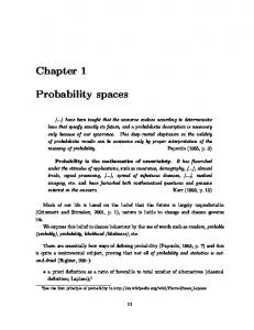
Alternatively, models of RT are often defined directly in terms of operations on random variables. Consider, for example, Donders’ method of subtraction in the detection task; if two experimental conditions differ by an additional decision stage, D, total response time may be conceived of as the sum of two random variables, D + R, where R is the time for responding to a high intensity stimulus. In the case of a mixture distribution, one may wonder whether or not it might also be possible to represent the observed RTs as the sum of two random variables H and L, say, or, more generally, if the observed RTs follow the distribution function of some Z(H, L), where Z is a measurable two-place function of H and L. In fact, the answer is negative and follows as a classic result from the theory of copulas (Nelsen, 2006), to be treated later in this chapter. Example 1.2 (Coupling for audiovisual interaction) In a classic study of intersensory facilitation, Hershenson (1962) compared reaction time to a moderately intense visual or acoustic stimulus to the RT when both stimuli were presented more or less simultaneously. Mean RT of a well-practiced subject to the sound (RTA , say) was approximately 120 ms, mean RT to the light (RTV ) about 160 ms. When both stimuli were presented synchronously, mean RT was still about 120 ms. Hershenson reasoned that intersensory facilitation could only occur if the “neural events” triggered by the visual and acoustic stimuli occurred simultaneously somewhere in the processing. That is, “physiological synchrony”, rather than “physical (stimulus) synchrony” was required. Thus, he presented bimodal stimuli with light leading sound giving the slower system a kind of “head start”. In the absence of interaction, reaction time to the bimodal stimulus with presentation of the acoustic delayed by τ ms, denoted as RTV τ A , is expected to increase linearly until the sound is delivered 40 ms after the light (the upper graph in Figure 1.1). Actual results, however, looked more like the lower graph in Figure 1.1 where maximal facilitation occurs at about physiological synchrony. Raab (1962) suggested an explanation in terms of a probability summation (or, race) mechanism: response time to the bimodal stimulus, RTV τ A , is considered to be the winner of a race between the processing times for the unimodal stimuli, i.e. RTV τ A ≡ min{RTV , RTA + τ }. It then follows for the expected values (mean RTs): E[RTV τ A ] = E[min{RTV , RTA + τ }] ≤ min{E[RTV ], E[RTA + τ ]}, a prediction that is consistent with the observed facilitation. It has later been shown that this prediction is not sufficient for explaining the observed

6

Contents

Figure 1.1 Bimodal (mean) reaction time to light and sound with interstimulus interval (ISI) and sound following light, RTV = 160 ms, RTA = 120 ms. Upper graph: prediction in absence of interaction, lower graph: observed mean RTs; data from Diederich and Colonius (1987).

amount of facilitation, and the discussion of how the effect should be modeled is still going on, attracting a lot of attention in both psychology and neuroscience. However, as already observed by Luce (1986, p. 130), the above inequality only makes sense if one adds the assumption that the three random variables RTV τ A , RTV , and RTA are jointly distributed. Existence of a joint distribution is not automatic because each variable relates to a different underlying probability space defined by the experimental condition: visual, auditory, or bimodal stimulus presentation. From the theory of coupling (Thorisson, 2000), constructing such a joint distribution is always possible by assuming stochastic independence of the random variables. However –and this is the main point of this example– independence is not the only coupling possibility, and alternative assumptions yielding distributions with certain dependency properties may be more appropriate to describe empirical data. Example 1.3 (Characterizing RT distributions: hazard function) Sometimes, a stochastic model can be shown to predict a specific parametric distribution, e.g. drawing on some asymptotic limit argument (central limit theorem or convergence to extreme-value distributions). It is often notori-

1.1 Introduction

7

ously difficult to tell apart two densities when only a histogram estimate from a finite sample is available. Figure 1.2 provides an example of two theoretically important distributions, the gamma and the inverse gaussian densities with identical means and standard deviations, where the rather similar shapes make it difficult to distinguish them on the basis of a histogram.

Figure 1.2 Inverse gaussian (dashed line) and gamma densities with identical mean (60 ms) and standard deviation (35 ms).

An alternative, but equivalent, representation of these distributions is terms of their hazard functions (see Section 1.10). The hazard function hX of random variable X with distribution function FX (x) and density fX (x) is defined as fX (x) hX (x) = . 1 − FX (x) As Figure 1.3 illustrates, the gamma hazard function is increasing with decreasing slope, whereas the inverse gaussian is first increasing and then decreasing. Although estimating hazard functions also has its intricacies (Kalbfleisch and Prentice, 2002), especially at the right tail, there is a better chance to tell the distributions apart based on estimates of the hazard function than on the density or distribution function. Still other methods to distinguish classes of distribution functions are based on the concept of quantile function (see Section 1.3.2), among them the method of delta plots, which has recently drawn the attention of researchers in RT modeling (Schwarz and Miller, 2012). Moreover, an underlying theme of this chapter is to provide tools for a model builder that do not depend on committing oneself to a particular parametric distribution assumption. We hope to convey in this chapter that even seemingly simple situations,

8

Contents

Figure 1.3 Hazard functions of the inverse gaussian (dashed line) and gamma distributions corresponding to the densities of Figure 1.2.

like the one described in Example 1.2, may require some careful consideration of the underlying probabilistic concepts. 1.1.2 Overview In trying to keep the chapter somewhat self-contained, the first part presents basic concepts of probability and stochastic processes, including some elementary notions of measure theory. Because of space limitations, some relevant topics had to be omitted (e.g., random walks, Markov chains) or are only mentioned in passing (e.g., martingale theory). For the same reason, statistical aspects are considered only when suggested by the context2 . Choosing what material to cover was guided by the specific requirements of the topics in the second, main part of the chapter. The second part begins with a brief introduction to the notion of exchangeability (with a reference to an application in vision) and its role in the celebrated “theorem of de Finetti”. An up-to-date presentation of quantile (density) functions follows, a notion that emerges in many areas including survival analysis. The latter topic, while central to RT analysis, has also found applications in diverse areas, like decision making and memory, and is treated next at some length, covering an important non-identifiability result. Next follow three related topics: order statistics, extreme values, and the theory of records. Whereas the first and, to a lesser degree, the second of these topics have become frequent tools in modeling psychological processes, the third one has not yet found the role that it arguably deserves. 2

For statistical issues of reaction time analysis, see the competent treatments by Van Zandt (2000, 2002); and Ulrich and Miller (1994), for discussing effects of truncation.

1.2 Basics

9

The method of coupling, briefly mentioned in introductory Example 1.2, is a classic tool of probability theory concerned with the construction of a joint probability space for previously unrelated random variables (or, more general random entities). Although it is being used in many parts of probability, e.g., Poisson approximation, and in simulation, there are not many systematic treatises of coupling and it is not even mentioned in many standard monographs of probability theory. We can only present the theory at a very introductory level here, but the expectation is that coupling will have to play an important conceptual role in psychological theorizing. For example, its relevance in defining ’selective influence/contextuality’ has been demonstrated in the work by Dzhafarov and colleagues (see also the chapter by Dzhafarov and Kujala in this volume). While coupling strives to construct a joint probability space, existence of a multivariate distribution is presumed in the next two sections. Fr´echet classes are multivariate distributions that have certain of their marginal distributions fixed. The issues are (i) to characterize upper and lower bounds for all elements of a given class and (ii) to determine conditions under which (bivariate or higher) margins with overlapping indices are compatible. Copula theory allows one to separate the dependency structure of a multivariate distribution from the specific univariate margins. This topic is pursued in the subsequent section presenting a brief overview of different types of multivariate dependence. Comparing uni- and multivariate distribution functions with respect to location and/or variability is the topic of the final section, stochastic orders. A few examples of applications of these concepts to issues in mathematical psychology are interspersed in the main text. Moreover, the comments and reference section at the end gives a number of references to further pertinent applications. 1.2 Basics Readers familiar with basic concepts of probability and stochastic processes, including some measure-theoretic terminology, may skip this first section of the chapter. 1.2.1 σ-algebra, probability space, independence, random variable, and distribution function A fundamental assumption of practically all models and methods of response time analysis is that the response latency measured in a given trial of a

10

Contents

reaction time task is the realization of a random variable. In order to discuss the consequences of treating response time as a random variable or, more generally, as a function of several random variables, some standard concepts of probability theory will first be introduced.3 Let Ω be an arbitrary set, often referred to as sample space or set of elementary outcomes of a random experiment, and F a system of subsets of Ω endowed with the properties of a σ-algebra (of events), i.e., (i) ∅ ∈ F ( “impossible” event ∅). (ii) If A ∈ F then also its complement: Ac ∈ F. S (iii) For a sequence of events {An ∈ F}n≥1 , then also ∞ n=1 An ∈ F The pair (Ω, F) is called measurable space. Let A be any collection of subsets of Ω. Since the power set, P(Ω), is a σ-algebra, it follows that there exists at least one σ-algebra containing A. Moreover, the intersection of any number of σ-algebras is again a σ-algebra. Thus, there exists a unique smallest σalgebra containing A, defined as the intersection of all σ-algebras containing A, called the σ-algebra generated by A and denoted as S(A). Definition 1.4 (Probability space) The triple (Ω, F, P ) is a probability space if Ω is a sample space with σ-algebra F such that P satisfies the following (Kolmogorov ) axioms: (1) For any A ∈ F, there exists a number P (A) ≥ 0; the probability of A. (2) P (Ω) = 1. (3) For any sequence of mutually disjoint events {An , n ≥ 1}, P(

∞ [ n=1

An ) =

∞ X

P (An ).

n=1

Then P is called probability measure, the elements of F are the measurable subsets of Ω, and the probability space (Ω, F, P ) is an example of measure spaces which may have measures other than P . Some easy to show consequences of the three axioms are, for measurable sets A, A1 , A2 , 1. 2. 3. 4. 3

P (Ac ) = 1 − P (A); P (∅) = 0; P (A1 ∪ A2 ) ≤ P (A1 ) + P (A2 ); A1 ⊂ A2 → P (A1 ) ≤ P (A2 ). Limits of space do not permit a completely systematic development here, so only a few of the most relevant topics will be covered in detail. For a more comprehensive treatment see the references in the final section (and Chapter 4 for a more general approach).

1.2 Basics

11

A set A ⊂ Ω is called a null set if there exists B ∈ F, such that B ⊃ A with P (B) = 0. In general, null sets need not be measurable. If they are, the probability space (Ω, F, P ) is called complete 4 . A property that holds everywhere except for those ω in a null set is said to hold (P -)almost everywhere (a.e.). Definition 1.5 (Independence) The events {Ak , 1 ≤ k ≤ n} are independent if, and only if, \  Y P Aik = P (Aik ), where intersections and products, respectively, are to be taken over all subsets of {1, 2, . . . , n}. The events {An , n ≥ 1} are independent if {Ak , 1 ≤ k ≤ n} are independent for all n. Definition 1.6 (Conditional probability) Let A and B be two events and suppose that P (A) > 0. The conditional probability of B given A is defined as P (A ∩ B) P (B|A) = . P (A) Remark 1.7 If A and B are independent, then P (B|A) = P (B). Moreover, P (·|A) with P (A) > 0 is a probability measure. Because 0 ≤ P (A ∩ B) ≤ P (A) = 0, null sets are independent of “everything”. The following statements about any subsets (events) of Ω, {Ak , 1 ≤ k ≤ n}, turn out to be very useful in many applications in response time analysis and are listed here for later reference. Remark 1.8 P

(Inclusion-exclusion formula) ! n n [ X X Ak = P (Ak ) − P (Ai ∩ Aj )

k=1

1≤i≤j≤n

k=1

+

X

P (Ai ∩ Aj ∩ Ak )

1≤i x2 ), for all x1 ≥ 0, x2 ≥ 0, t ≥ 0, and BVE is the only bivariate distribution with exponential marginals possessing this property; (c) BVE distribution is a mixture of an absolutely continuous distribution Fac (x1 , x2 ) and a singular distribution Fcs (x1 , x2 ): λ1 + λ2 ¯ λ12 ¯ F¯ (x1 , x2 ) = Fac (x1 , x2 ) + Fs (x1 , x2 ), λ λ where F¯s (x1 , x2 ) = exp[−λ max(x1 , x2 )] and, F¯ac (x1 , x2 ) =

λ exp[−λ1 x1 − λ2 x2 − λ12 max(x1 , x2 )] λ1 + λ2 λ12 − exp[−λ max(x1 , x2 )]. λ1 + λ2

1.2.3 Expectation, other moments, and tail probabilities The consistency of the following definitions is based on the theory of Lebesgue integration and the Riemann-Stieltjes integral (some knowledge of which is presupposed here). Definition 1.29 (Expected value) Let X be a real-valued random variable

20

Contents

on a probability space (Ω, F, P ). The expected value of X (or mean of X) is the integral of X with respect to measure P : Z Z EX = X(ω) dP (ω) = X dP. Ω

For X ≥ 0, E X is always defined (it may be infinite); for the general X, E X is defined if at least one of E X + or E X − is finite8 , in which case E X = E X + − E X −; if both values are finite, that is, if E |X| < ∞, we say that X is integrable. Let X, Y be integrable random variables. The following are basic consequences of the (integral) definition of expected value: 1. 2. 3. 4. 5. 6. 7. 8.

If X = 0 a.s., then E X = 0; |X| < ∞ a.s., that is, P (|X| < ∞) = 1; If E X > 0, then P (X > 0) > 0; Linearity: E (aX + bY ) = aE X + bE Y , for any a, b ∈ 0, if: 1. N (0) = 0; 2. N (t) has independent increments; 3. the number of events in any interval of length t is Poisson distributed with mean λt; that is, for all s, t ≥ 0, P (N (t + s) − N (s) = n) = exp[−λt]

(λt)n , n = 0, 1, . . . n!

Obviously, a Poisson process has stationary increments. Moreover, E[N (t)] = λt. For the interarrival times, one has Proposition 1.41 The interarrival times {Xn , n ≥ 1} of a Poisson process with rate λ are independent identically distributed (i.i.d.) exponential random variables with mean 1/λ. Proof

Obviously, P (X1 > t) = P (N (t) = 0) = exp[−λt],

so X1 has the exponential distribution. Then P (X2 > t | X1 = s) =P (no events in (s, s + t] | X1 = s) =P (no events in (s, s + t]) (by independent increments) = exp[−λt] (by stationary increments).

Given the memoryless property of the exponential, the last result shows that the Poisson process probabilistically restarts itself at any point in time. For the waiting time until the nth event of the Poisson process, the density is (λt)n−1 f (t) = λ exp[−λt] , t ≥ 0, (1.3) (n − 1)! i.e., the gamma density, Gamma(n, λ). This follows using convolution (or

1.2 Basics

27

moment generating functions), but it can also be derived by appealing to the following logical equivalence: N (t) ≥ n ⇔ Sn ≤ t. Hence, P (Sn ≤ t) = P (N (t) ≥ n) ∞ X (λt)j = exp[−λt] , j!

(1.4) (1.5)

j=n

which upon differentiation yields the gamma density. Note that a function f is said to be o(h) if f (h) = 0. h→0 h lim

One alternative definition of the Poisson process is contained the following: Proposition 1.42 The counting process {N (t), t ≥ 0} is a Poisson process with rate λ, λ > 0, if and only if: 1. 2. 3. 4.

N (0) = 0; the process has stationary and independent increments; P (N (h) = 1) = λh + o(h); P (N (h) ≥ 2) = o(h).

Proof

(see Ross, 1983, p. 32–34) The non-homogeneous Poisson process

Dropping the assumption of stationarity leads to a generalization of the Poisson process that also plays an important role in certain RT model classes, the counter models. Definition 1.43 The counting process {N (t), t ≥ 0} is a nonstationary, or non-homogeneous Poisson process with intensity function λ(t), t ≥ 0, if: 1. 2. 3. 4.

N (0) = 0; {N (t), t ≥ 0} has independent increments; P (N (t + h) − N (t) = 1) = λ(t)h + o(h); P (N (t + h) − N (t)) ≥ 2) = o(h). Letting Zt m(t) =

λ(s) ds, 0

28

Contents

it can be shown that P (N (t + s) − N (t) = n) = exp[−(m(t + s)−m(t))][m(t + s) − m(t)]n /n!, n = 0, 1, 2 . . . , (1.6) that is, N (t + s) − N (t) is Poisson distributed with mean m(t + s) − m(t). A non-homogeneous Poisson process allows for the possibility that events may be more likely to occur at certain times than at other times. Such a process can be interpreted as being a random sample from a homogeneous Poisson process, if function λ(t) is bounded, in the following sense (p. 46 Ross, 1983): Let λ(t) ≤ λ, for all t ≥ 0; suppose that an event of the process is counted with probability λ(t)/λ, then the process of counted events is a non-homogeneous Poisson process with intensity function λ(t): Properties 1, 2, and 3 of Definition 1.43 follow since they also hold for the homogenous Poisson process. Property 4 follows since P (one counted event in (t, t + h)) = P (one event in (t, t + h))

λ(t) + o(h) λ

λ(t) + o(h) λ = λ(t)h + o(h). = λh

An example of this process in the context of record values is presented at the end of Section 1.3.4.

1.3 Specific topics 1.3.1 Exchangeability When stochastic independence does not hold, the multivariate distribution of a random vector can be a very complicated object that is difficult to analyze. If the distribution is exchangeable, however, the associated distribution function F can often be simplifed and written in a quite compact form. Exchangeability intuitively means that the dependence structure between the components of a random vector is completely symmetric and does not depend on the ordering of the components (Mai and Scherer, 2012, p. 39 pp.). Definition 1.44 (Exchangeability) Random variables X1 , . . . , Xn are exchangeable if, for the random vector (X1 , . . . , Xn ), (X1 , . . . , Xn ) =d (Xi1 , . . . , Xin )

1.3 Specific topics

29

for all permutations (i1 , . . . , in ) of the subscripts (1, . . . , n). Furthermore, an infinite sequence of random variables X1 , X2 , . . . is exchangeable if any finite subsequence of X1 , X2 , . . . is exchangeable. Notice that a subset of exchangeable random variables can be shown to be exchangeable. Moreover, any collection of independent identically distributed random variables is exchangeable. The distribution function of a random vector of exchangeable random variables is invariant with respect to permutations of its arguments. The following proposition shows that the correlation structure of a finite collection of exchangeable random variables is limited: Proposition 1.45 Let X1 , . . . , Xn be exchangeable with existing pairwise correlation coefficients ρ(Xi , Xj ) = ρ, i 6= j. Then ρ ≥ −1/(n − 1). Proof Without loss of generality, we scale the variables such that EZi = 0 and EZi2 = 1. Then X X X 0 ≤ E( Zi )2 = EZi2 + EZi Zj = n + n(n − 1)ρ, i

i6=j

from which the inequality follows immediately. Note that this also implies that ρ ≥ 0, for an infinite sequence of exchangeable random variables. The assumption that a finite number of random variables are exchangeable is significantly different from the assumption that they are a finite segment of an infinite sequence of exchangeable random variables (for a simple example, see Galambos, 1978, pp. 127–8). The most important result for exchangeable random variables is known as “de Finetti’s theorem”, which is often stated in words such as “An infinite exchangeable sequence is a mixture of i.i.d. sequences”. The precise result, however, requires measure theoretic tools like random measures. First, let us consider the ”Bayesian viewpoint” of sampling. Let X1 , . . . , Xn be observations on a random variable with distribution function F (x, θ), where θ is a random variable whose probability function p is assumed to be independent of the Xj . For a given value of θ, the Xj are assumed to be i.i.d. Thus, the distribution of the sample is   Z Y n n Y P (X1 ≤ x1 , . . . , Xn ≤ xn ) = F (xj , θ)p(θ) dθ = E  F (xj , θ) . j=1

j=1

(1.7) Obviously, X1 , . . . , Xn are exchangeable random variables. The following theorem addresses the converse of this statement.

30

Contents

Theorem 1.46 (“de Finetti’s theorem”) An infinite sequence X1 , X2 , . . . of random variables on a probability space (Ω, F, P ) is exchangeable if, and only if, there is a sub-σ-algebra G ⊂ F such that, given G, X1 , X2 , . . . are a.s. independent and identically distributed, that is, P (X1 ≤ x1 , . . . , Xn ≤ xn | G) =

n Y

P (X1 ≤ xj | G) a.s.,

j=1

for all x1 , . . . xn ∈ 0 and λ > 0. Then Q(u) = λ−1 (− log(1 − u)). If f (x) is the probability density function of X, then f (Q(u)) is called the density quantile function. The derivative of Q(u), i.e., q(u) = Q0 (u), is known as the quantile density function of X. Differentiating F (Q(u)) = u, we find q(u)f (Q(u)) = 1.

(1.9)

We collect a number of properties of quantile functions: 1. Q(u) is non-decreasing on (0, 1) with Q(F (x)) ≤ x, for all −∞ < x < +∞ for which 0 < F (x) < 1; 2. F (Q(u)) ≥ u, for any 0 < u < 1; 3. Q(u) is continuous from the left, or Q(u−) = Q(u); 4. Q(u+) = inf{x : F (x) > u} so that Q(u) has limits from above; 5. any jumps of F (x) are flat points of Q(u) and flat points of F (x) are jumps of Q(u); 6. a non-decreasing function of a quantile function is a quantile function. 7. the sum of two quantile functions is again a quantile function; 8. two quantile density functions, when added, produce another quantile density function; 9. if X has quantile function Q(u), then 1/X has quantile function 1/Q(1−u). The following simple but fundamental fact shows that any distribution function can be conceived as arising from the uniform distribution transformed by Q(u): Proposition 1.49 If U is a uniform random variable over [0, 1], then X = Q(U ) has its distribution function as F (x). Proof P (Q(U ) ≤ x) = P (U ≤ F (x)) = F (x).

32

Contents

1.3.3 Survival analysis Survival function and hazard function Given that time is a central notion in survival analysis, actuarial, and reliability theory it is not surprising that many concepts from these fields have an important role to play in the analysis of psychological processes as well. In those contexts, realization of a random variable is interpreted as a “critical event”, e.g., death of an individual or breakdown of a system of components. Let FX (x) be the distribution function of random variable X; then SX (x) = 1 − FX (x) = P (X > x), for x ∈ x) ∆x

For P (X > x) > 0, P (x < X ≤ x + ∆x) 1 − FX (x) FX (x + ∆x) − FX (x) = , 1 − FX (x)

P (x < X ≤ x + ∆x | X > x) =

whence it follows that

(1.11)

1.3 Specific topics

lim

∆x↓0

33

P (x < X ≤ x + ∆x | X > x) 1 FX (x + ∆x) − FX (x) = lim ∆x 1 − FX (x) ∆x↓0 ∆x 1 = fX (x) SX (x)

Thus, for “sufficiently” small ∆x, the product hX (x) · ∆x can be interpreted as the probability of the “critical event” occurring in the next instant of time given it has not yet occurred. Or, written with the o() function: P (x < X ≤ x + ∆x | X > x) = hX (x)∆x + o(∆x). The following conditions have been shown to be necessary and sufficient for a function h(x) to be the hazard function of some distribution (see Marshall and Olkin, 2007). 1. 2. 3. 4.

≥ 0; Rh(x) x h(t) dt < +∞, for some x > 0; R0+∞ R0x h(t) dt = +∞; 0 h(t) dt = +∞ implies h(y) = +∞, for every y > x.

It is easy to see that the exponential distribution with parameter λ > 0 corresponds to a constant hazard function, hX (x) = λ expressing the “lack of memory” property of that distribution. A related quantity is the cumulative (or, integrated ) hazard function H(x) defined as Z x

h(t) dt = − log S(x).

H(x) = 0

Thus,  Z S(x) = exp −

x

 h(t) dt ,

0

showing that the distribution function can be regained from the hazard function. Example 1.52 (Hazard function of the minimum) Let X1 , X2 , . . . , Xn be independent random variables, defined on a common probability space, and Z = min(X1 , X2 , . . . , Xn ). Then SZ (x) = P (Z > z) = P (X1 > x, X2 > x, . . . , Xn > x) = SX1 (x) . . . SXn (x).

34

Contents

Logarithmic differentiation leads to hZ (x) = hX1 (x) + . . . + hXn (x). In reliability theory, this model constitutes a series system with n independent components, each having possibly different life distributions: the system breaks down as soon as any of the components does, i.e. the “hazards” cumulate with the number of components involved. For example, the Marshall-Olkin BVE distribution (Example 1.28) can be interpreted to describe a series system exposed to three independent “fatal” break-downs with a hazard function λ = λ1 + λ2 + λ12 . Hazard quantile function For many distributions, like the normal, the corresponding quantile function cannot be obtained in closed form, and the solution of F (x) = u must be obtained numerically. Similarly, there are quantile functions for which no closed-form expressions for F (x) exists. In that case, analyzing the distribution via its hazard function is of limited use, and a translation in terms of quantile functions is more promising (Nair et al., 2013). We assume an absolutely continuous F (x) so that all quantile related functions are well defined. Setting x = Q(u) in Equation 1.10 and using the relationship f (Q(u)) = [q(u)]−1 , the hazard quantile function is defined as H(u) = h(Q(u)) = [(1 − u)q(u)]−1 .

(1.12)

From q(u) = [(1 − u)H(u)]−1 , we have Z u dv Q(u) = . (1 − v)H(v) 0 The following example illustrates these notions. Example 1.53

(Nair et al., 2013, p. 47) Taking Q(u) = uθ+1 (1 + θ(1 − u)), θ > 0,

we have q(u) = uθ [1 + θ(θ + 1)(1 − u)], and so H(u) = [(1 − u)uθ (1 + θ(θ + 1)(1 − u))]−1 . Note that there is no analytic solution for x = Q(u) that gives F (x) in terms of x.

1.3 Specific topics

35

Competing risks models: hazard-based approach An extension of the hazard function concept, relevant for response times involving, e.g., a choice between different alternatives, is to assume that not only the time of breakdown but also its cause C are observable. We define a joint sub-distribution function F for (X, C), with X the time of breakdown and C its cause, where C = 1, . . . , p, a (small) number of labels for the different causes: F (x, j) = P (X ≤ x, C = j), and a sub-survival distribution defined as S(x, j) = P (X > x, C = j). Then, F (x, j) + S(x, j) = pj = P (C = j). Thus, F (x, j) is not a proper distribution function because it only reaches the values pj instead of 1 when P x → +∞. It is assumed implicitly that pj > 0 and p1 pj = 1. Note that S(x, j) is not, in general, equal to the probability that X > x for breakdowns of type j; rather, that is the conditional probability P (X > x | C = j) = S(x, j)/pj . For continuous X, the sub-density function is f (x, j) = −dS(x, j)/dx. The marginal survival function and marginal density of X are calculated from

S(x) =

p X

S(x, j) and f (x) = −dS(x)/dx =

j=1

p X

f (x, j).

(1.13)

j=1

Next, one defines the hazard function for breakdown from cause j, in the presence of all risks, in similar fashion as the overall hazard function: Definition 1.54 (Sub-hazard function) The sub-hazard function (for breakdown from cause j in the presence of all risks 1, . . . , p) is P (x < X ≤ x + ∆x, C = j | X > x) ∆x↓0 ∆x S(x, j) − S(x + ∆x, j) = lim (∆x)−1 ∆x↓0 S(x) f (x, j) = . S(x)

h(x, j) = lim

(1.14)

Sometimes, h(x, j) is called cause-specific or crude hazard function. The P overall hazard function13 is h(x) = pj=1 h(x, j). 13

Dropping subscript X here for simplicity.

36

Contents

Example 1.55 (Weibull competing risks model) One can specify a Weibull competing risks model by assuming sub-hazard functions of the form −αj αj −1

h(x, j) = αj βj

x

,

with αj , βj > 0. The overall hazard function then is h(x) =

p X

−αj αj −1

αj βj

x

,

j=1

and the marginal survival function follows as  x    p  Z   X  (x/βj )αj . S(x) = exp − h(y) dy = exp −     0

j=1

In view of Example 1.52, this shows that X has the distribution of min(X1 , . . . , Xp ), the Xj being independent Weibull variates with parameters (αj , βj ). The sub-densities f (x, j) can be obtained as h(x, j)S(x), but integration of this in order to calculate the sub-survival distributions is generally intractable. A special type of competing risks model emerges when proportionality of hazards is assumed, that is, when h(x, j)/h(x) does not dependent on x for each j. It means that, over time, the instantaneous risk of a “critical event” occurring may increase or decrease, but the relative risks of the various causes remain invariant. The meaning of the assumption is captured more precisely by the following lemma (for proof see, e.g., Kochar and Proschan, 1991). Lemma 1.56 (Independence of time and cause) are equivalent:

The following conditions

1. h(x, j)/h(x) does not dependent on x for all j (proportionality of hazards); 2. the time and cause of breakdown are independent; 3. h(x, j)/h(x, k) is independent of x, for all j and k. In this case, h(x, j) = pj h(x) or, equivalently, f (x, j) = pj f (x) or F (x, j) = pj F (x). The second condition in the lemma means that breakdown during some particular period does not make it any more or less likely to be from cause j than breakdown in some other period. Example 1.57

−αj αj −1 x

(Weibull sub-hazards) With h(x, j) = αj βj

(see

1.3 Specific topics

37

Example 1.55) proportional hazards only holds if the αj are all equal, say P to α. Let β + = pj=1 βj−α ; in this case, S(x) = exp[−β + xα ] and f (x, j) = h(x, j)S(x) = αβj−α xα−1 exp[−β + xα ]. With πj = βj−α /β + , the sub-survival distribution is S(x, j) = πj exp[−β + xα ], showing that this is a mixture model in which pj = P (C = j) = πj and P (X > x | C = j) = P (X > x) = exp[−β + xα ], i.e., time and cause of breakdown are stochastically independent. Competing risks models: latent-failure times approach While the sub-hazard function introduced above has become the core concept of competing risks modeling, the more traditional approach was based on assuming existence of a latent failure time associated with each of the p potential causes of breakdown. If Xj represents the time to system failure from cause j (j = 1, . . . , p), the smallest Xj determines the time to overall system failure, and its index is the cause of failure C. This is the prototype of the concept of parallel processing and, as such, central to reaction time modeling as well. For the latent failure times we assume a vector X = (X1 , . . . , Xp ) with absolutely continuous survival function G(x) = P (X > x) and marginal survival distributions Gj (x) = P (Xj > x). The latent failure times are of course not observable, nor are the marginal hazard functions hj (x) = −d log Gj (x)/dx. However, we clearly must have an identity between G(x) and the marginal survival function S(x) introduced in Equation 1.13, G(x1p ) = S(x),

(1.15)

where 1p 0 = (1, . . . , 1) of length p. It is then easy to show (see, e.g., Crowder, 2012, p. 236) that the sub-densities can be calculated from the joint survival distribution of the latent failure times as f (x, j) = [−∂G(x)/∂xj ]x1p , and the sub-hazards follow as h(x, j) = [−∂ log G(x)/∂xj ]x1p ,

38

Contents

where the notation [. . .]x1p indicates that the enclosed function is to be evaluated at x = (x, . . . , x). Independent risks Historically, the main aim of competing risks analysis was to estimate the marginal survival distributions Gj (x) from the subsurvival distributions S(x, j). While this is not possible in general, except by specifying a fully parametric model for G(x), it can also be done by assuming that the risks act independently. In particular, it can be shown (see Crowder, 2012, p. 245) that the set of sub-hazard functions h(x, j) determines the set of marginals Gj (x) via   Z x h(y, j) dy . Gj (x) = exp − 0

Without making such strong assumptions, it is still possible to derive some bounds for Gj (x) in terms of S(x, j). Obviously, S(x, j) = P (Xj > x, C = j) ≤ P (Xj > x) = Gj (x). More refined bounds are derived in Peterson (1976): Let y = max{x1 , . . . , xp }. Then p X j=1

S(y, j) ≤ G(x) ≤

p X

S(xj , j).

(1.16)

j=1

Setting xk = x and all other xj = 0 yields, for x > 0 and each k, p X

S(x, j) ≤ Gk (x) ≤ S(x, k) + (1 − pk ).

(1.17)

j=1

These bounds cannot be improved because they are attainable by particular distributions, and they may be not very restrictive; that is, even knowing the S(x, j) quite well may not suffice to say much about G(x) or Gj (x). This finding is echoed in some general non-identifiability results considered next. Some non-identifiability results A basic result, much discussed in the competing risks literature, is (for proof, see Tsiatis, 1975): Proposition 1.58 (Tsiatis’ Theorem) For any arbitrary, absolutely continuous survival function G(x) with dependent risks and sub-survival distributions S(x, j), there exist a unique “proxy model” with independent risks

1.3 Specific topics

39

yielding identical S(x, j). It is defined by G∗ (x) =

p Y

G∗j (xj ), where G∗j (xj ) = exp{−

Z

x

h(y, j)dy}

(1.18)

0

j=1

and the sub-hazard function h(x, j) derives from the given S(x, j). The following example illustrates why this non-identifiability is seen as a problem. Example 1.59 (Gumbel’s bivariate exponential distribution) survival distribution is

The joint

G(x) = exp[−λ1 x1 − λ2 x2 − νx1 x2 ], with λ1 > 0 and λ2 > 0 and 0 ≤ ν ≤ λ1 λ2 . Parameter ν controls dependence: ν = 0 implies stochastic independence between X1 and X2 . The univariate marginals are P (Xj > xj ) = Gj (xj ) = exp[−λj xj ]. Then the marginal survival distribution is S(x) = exp[−(λ1 + λ2 )x − νx2 ] and the sub-hazard functions are h(x, j) = λj + νx, j = 1, 2. From the Tsiatis theorem, the proxy model has  Z x  ∗ Gj (x) = exp − (λj + νy)dy = exp[−(λj x + νx2 /2)] 0

G∗ (x) = exp[−(λ1 x1 + νx21 /2) − (λ2 x2 + νx22 /2)]. Thus, to make predictions about Xj one can either use Gj (x) or G∗j (x), and the results will not be the same (except if ν = 0). One cannot tell which one is correct from just (X, C) data. There are many refinements of Tsiatis’ theorem and related results (see e.g., Crowder, 2012) and, ultimately, the latent failure times approach in survival analysis has been superseded by the concept of sub-hazard function within the more general context of counting processes (Aalen et al., 2008).

1.3.4 Order statistics, extreme values, and records The concept of order statistics plays a major role in RT models with a parallel processing architecture. Moreover, several theories of learning, memory, and automaticity have drawn upon concepts from the asymptotic theory of specific order statistics, the extreme values. Finally, we briefly treat theory of record values, a well developed statistical area which, strangely enough, has not yet played a significant role in RT modeling.

40

Contents

Order statistics Suppose that (X1 , X2 . . . , Xn ) are n jointly distributed random variables. The corresponding order statistics are the Xi ’s arranged in ascending order of magnitude, denoted by X1:n ≤ X2:n ≤ . . . ≤ Xn:n . In general, the Xi are assumed to be i.i.d. random variables with F (x) = P (Xi ≤ x), i = 1, . . . n, so that (X1 , X2 . . . , Xn ) can be considered as random sample from a population with distribution function F (x). The distribution function of Xi:n is obtained realizing that Fi:n (x) = P (Xi:n ≤ x) = P (at least i of X1 , X2 , . . . , Xn are less than or equal to x) n X = P (exactly r of X1 , X2 , . . . , Xn are less than or equal to x ) r=i n   X n = [F (x)]r [1 − F (x)]n−r , −∞ < x < +∞. r

(1.19)

r=i

For i = n, this gives Fn:n (x) = P (max(X1 , . . . , Xn ) ≤ x) = [F (x)]n , and for i = 1, F1:n (x) = P (min(X1 , . . . , Xn ) ≤ x) = 1 − [1 − F (x)]n . Assuming existence of the probability density for (X1 , X2 . . . , Xn ), the joint density for all n order statistics – which, of course, are no longer stochastically independent – is derived as follows (Arnold et al., 1992, p. 10). Given the realizations of the n order statistics to be x1:n < x2:n < · · · < xn:n , the original variables Xi are restrained to take on the values xi:n (i = 1, 2, . . . , n), which by symmetry assigns equal probability for each of the n! permutations of (1, 2, . . . , n). Hence, the joint density function of all n order statistics is f1,2,...,n:n (x1 , x2 , . . . , xn ) = n!

n Y

f (xr ), −∞ < x1 < x2 < · · · < xn < +∞.

r=1

The marginal density of Xi:n is obtained by integrating out the remaining n − 1 variables, yielding n! [F (x)]i−1 [1 − F (x)]n−i f (x), −∞ < x < +∞. (i − 1)!(n − i)! (1.20) It is relatively straightforward to compute the joint density and the distribution function of any two order statistics (see Arnold et al., 1992). fi:n (x) =

1.3 Specific topics

41

Let U1 , U2 , . . . , Un be a random sample from the standard uniform distribution (i.e., over [0, 1]) and X1 , X2 , . . . , Xn be a random sample from a population with distribution function F (x), and U1:n ≤ U2:n ≤ · · · ≤ Un:n and X1:n ≤ X2:n ≤ · · · ≤ Xn:n the corresponding order statistics. For a continuous distribution function F (x), the probability integral transformation U = F (X) produces a standard uniform distribution. Thus, for continuous F (x), F (Xi:n ) =d Ui:n ,

i = 1, 2, . . . n.

Moreover, it is easy to verify that, for quantile function Q(u) ≡ F −1 (u), one has Q(Ui ) =d Xi ,

i = 1, 2, . . . n.

Since Q is non-decreasing, it immediately follows that Q(Ui:n ) =d Xi:n ,

i = 1, 2, . . . n.

(1.21)

This implies simple forms for the quantile functions of the extreme order statistics, Qn and Q1 , 1/n Qn (un ) = Q(u1/n ], n ) and Q1 (u1 ) = Q[1 − (1 − u1 )

(1.22)

for the maximum and the minimum statistic, respectively. Moments of order statistics can often be obtained from the marginal den(m) sity (Equation 1.20). Writing µi:n for the m-th moment of Xi:n , (m) µi:n

+∞ Z xm [F (x)]i−1 [1 − F (x)]n−i f (x) dx,

n! = (i − 1)!(n − i)!

(1.23)

−∞

1 ≤ i ≤ n, m = 1, 2, . . . . Using relation (1.21), this can be written more compactly as (m) µi:n

n! = (i − 1)!(n − i)!

Z1

[F −1 (u)]m ui−1 (1 − u)n−i du,

(1.24)

0

1 ≤ i ≤ n, m = 1, 2, . . . The computation of various moments of order statistics can be reduced drawing upon various identities and recurrence relations. Consider the obvious identity n n X X m = Xim , m ≥ 1. Xi:n i=1

i=1

42

Contents

Taking expectation on both sides yields n X

(m)

(m)

µi:n = nEX m = nµ1:1 , m ≥ 1.

(1.25)

i=1

An interesting recurrence relation, termed triangle rule, is easily derived using Equation 1.24 (see Arnold et al., 1992, p. 112): For 1 ≤ i ≤ n − 1 and m = 1, 2 . . ., (m)

(m)

(m)

iµi+1:n + (n − i)µi:n = nµi:n−1 .

(1.26)

This relation shows that it is enough to evaluate the mth moment of a single order statistic in a sample of size n if these moments in samples of size less than n are already available. Many other recurrence relations, also including product moments and covariances of order statistics, are known and can be used not only to reduce the amount of computation (if these quantities have to be determined by numerical procedures) but also to provide simple checks of the accuracy of these computations (Arnold et al., 1992). Characterization of distributions by order statistics. Given that a distribution F is known, it is clear that the distributions Fi:n are completely determined, for every i and n. The interesting question is to what extent does knowledge of some properties of the distribution of an order statistic determine the parent distribution? Clearly, the distribution of Xn:n determines F completely since Fn:n (x) = [F (x)]n for every x, so that F (x) = [Fn:n (x)]1/n . It turns out that, assuming the moments are finite, equality of the first moments of maxima, 0 EXn:n = EXn:n ,

n = 1, 2 . . . ,

is sufficient to infer equality of the underlying parent distributions F (x) and F 0 (x) (see Arnold et al., 1992, p. 145). Moreover, distributional relations between order statistics can be drawn upon in order to characterize the underlying distribution. For example, straightforward computation yields that for a sample of size n from an exponentially distributed population, nX1:n =d X1:1 , for n = 1, 2, . . . .

(1.27)

Notably, it has been shown (Desu, 1971) that the exponential is the only nondegenerate distribution satisfying the above relation. From this, a characterization of the Weibull is obtained as well:

1.3 Specific topics

Example 1.60 (“Power Law of Practice”)

43

Let, for α > 0,

F (x) = 1 − exp[−xα ]; then, W = X α is a unit exponential variable (i.e., λ = 1) and Equation 1.27 implies the following characterization of the Weibull: n1/α X1:n =d X1:1 , for n = 1, 2, . . . .

(1.28)

At the level of expectations, EX1:n = n−1/α EX. This has been termed the “power law of practice” (Newell and Rosenbloom, 1981): the time taken to perform a certain task decreases as a power function of practice (indexed by n). This is the basis of G. Logan’s “theory of automaticity” (Logan, 1988, 1992, 1995) postulating Weibull-shaped RT distributions (see Colonius, 1995, for a comment on the theoretical foundations). Extreme value statistics The behavior of extreme order statistics, that is, of the maximum and minimum of a sample when sample size n goes to infinity, has attracted the attention of RT model builders, in particular in the context of investigating parallel processing architectures. Only a few results of this active area of statistical research will be considered here. For the underlying distribution function F , its right, or upper, endpoint is defined as ω(F ) = sup{x|F (x) < 1}. Note that ω(F ) is either +∞ or finite. Then the distribution of the maximum, Fn:n (x) = P (Xn:n ≤ x) = [F (x)]n , clearly converges to zero, for x < ω(F ), and to 1, for x ≥ ω(F ). Hence, in order to obtain a nondegenerate limit distribution, a normalization is necessary. Suppose there exists sequences of constants bn > 0 and an real (n = 1, 2, . . .) such that Xn:n − an bn has a nondegenerate limit distribution, or extreme value distribution, as n → +∞, i.e., lim F n (an + bn x) = G(x),

n→+∞

(1.29)

44

Contents

for every point x where G is continuous, and G a nondegenerate distribution function14 . A distribution function F satisfying Equation 1.29 is said to be in the domain of maximal attraction of a nondegenerate distribution function G, and we will write F ∈ D(G). Two distribution functions F1 and F2 are defined to be of the same type if there exist constants a0 and b0 > 0 such that F1 (a0 + b0 x) = F2 (x). It can be shown that (i) the choice of the norming constants is not unique and (ii) a distribution function cannot be in the domain of maximal attraction of more than one type of distribution. The main theme of extreme value statistics is to identify all extreme value distributions and their domains of attraction and to characterize necessary and/or sufficient conditions for convergence. Before a general result is presented, let us consider the asymptotic behavior for a special case. Example 1.61 Let Xn:n be the maximum of a sample from the exponential distribution with rate equal to λ. Then, ( (1 − exp[−(λx + log n)])n , if x > −λ−1 log n P (Xn:n − λ−1 log n ≤ x) = 0, if x ≤ −λ−1 log n = (1 − exp[−λx]/n)n , → exp[− exp[−λx]],

for x > −λ−1 log n −∞ < x < ∞,

as n → +∞. Possible limiting distributions for the sample maximum. The classic result on the limiting distributions, already described in Frech´et (1927) and Fisher and Tippett (1928), is the following: Theorem 1.62 If Equation 1.29 holds, the limiting distribution function G of an appropriately normalized sample maximum is one of the following types: ( 0, x≤0 G1 (x; α) = (1.30) −α exp[−x ], x > 0; α > 0 ( exp[−(−x)α ], x < 0; α > 0 G2 (x; α) = (1.31) 1, x≥0 G3 (x; α) = exp[− exp(−x)], 14

−∞ < x < +∞

Note that convergence here is convergence “in probability”, or “weak” convergence.

(1.32)

1.3 Specific topics

45

Distribution G1 is referred to as the Frech´et type, G2 as the Weibull type, and G3 as the extreme value or Gumbel distribution. Parameter α occurring in G1 and G2 is related to the tail behavior of the parent distribution F . It follows from the theorem that if F is in the maximal domain of attraction of some G, F ∈ D(G), then G is either G1 , G2 , or G3 . Necessary and sufficient conditions on F to be in the domain of attraction of G1 , G2 , or G3 , respectively, have been given in Gnedenko (1943). Since these are often difficult to verify Arnold et al. (1992, pp. 210–212), here we list sufficient conditions for weak convergence due to von Mises (1936): Proposition 1.63 Let F be an absolutely continuous distribution function and let h(x) be the corresponding hazard function. 1. If h(x) > 0 for large x and for some α > 0, lim x h(x) = α,

x→+∞

then F ∈ D(G1 (x; α)). Possible choices for the norming constants are an = 0 and bn = F −1 (1 − n−1 ). 2. If F −1 (1) < ∞ and for some α > 0, lim

(F −1 (1) − x)h(x) = α,

x→F −1 (1)

then F ∈ D(G2 (x; α)). Possible choices for the norming constants are an = F −1 (1) and bn = F −1 (1) − F −1 (1 − n−1 ). 3. Suppose h(x) is nonzero and is differentiable for x close to F −1 (1) or, for large x, if F −1 (1) = +∞. Then, F ∈ D(G3 ) if   d 1 lim = 0. h(x) x→F −1 (1) dx Possible choices for the norming constants are an = F −1 (1 − n−1 ) and bn = [nf (an )]−1 . Limiting distributions for sample minima. This case can be derived technically from the analysis of sample maxima, since the sample minimum from distribution F has the same distribution as the negative of the sample maximum from distribution F ∗ , where F ∗ (x) = 1 − F (−x). We sketch some of the results for completeness here. For parent distribution F one defines the left, or lower endpoint as α(F ) = inf{x : F (x) > 0}.

46

Contents

Note that α(F ) is either −∞ or finite. Then the distribution of the minimum, F1:n (x) = P (X1:n ≤ x) = 1 − [1 − F (x)]n , clearly converges to one, for x > α(F ), and to zero, for x ≤ α(F ). The theorem paralleling Theorem 1.62 then is Theorem 1.64 Suppose there exist constants a∗n and b∗n > 0 and a nondegenerate distribution function G∗ such that lim 1 − [1 − F (a∗n + b∗n x)]n = G∗ (x)

n→+∞

for every point x where G∗ is continuous, then G∗ must be one of the following types: 1. G∗1 (x; α) = 1 − G1 (−x; α), 2. G∗2 (x; α) = 1 − G2 (−x; α), 3. G∗3 (x) = 1 − G3 (−x), where G1 , G2 , and G3 are the distributions given in Theorem 1.62. Necessary and/or sufficient conditions on F to be in the domain of (minimal) attraction of G1 , G2 , or G3 , respectively, can be found e.g., in Arnold et al. (1992, pp. 213-214). Let us state some important practical implications of these results on asymptotic behavior: - Only three distributions (Fr´echet, Weibull, and extreme value/Gumbel) can occur as limit distributions of independent sample maxima or minima. - Although there exist parent distributions such that the limit does not exist, for most continuous distributions in practice one of them actually occurs. - A parent distribution with non-finite endpoint in the tail of interest cannot lie in a Weibull type domain of attraction. - A parent distribution with finite endpoint in the tail of interest cannot lie in a Fr´echet type domain of attraction. One important problem with practical implications is the speed of convergence to the limit distributions. It has been observed that, e.g. in the case of the maximum of standard normally distributed random variables, convergence to the extreme value distribution G3 is extremely slow and that Fn (an + bn x)n can be closer to a suitably chosen Weibull distribution G2 even for very large n. In determining the sample size required for the application of the asymptotic theory, estimates of the error of approximation

1.3 Specific topics

47

do not depend on x since the convergence is uniform in x. They do depend, however, on the choice of the norming constants (for more details, see Galambos, 1978, pp. 111–116). Because of this so called penultimate approximation, diagnosing the type of limit distribution even from rather large empirical samples may be problematic (see also the discussion in Colonius, 1995; Logan, 1995). Record values The theory of records should not be seen as a special topic of order statistics, but their study parallels the study of order statistics in many ways. In particular, things that are relatively easy for order statistics are also feasible for records, and things that are difficult for order statistics are equally or more difficult for records. Compared to order statistics, there are not too many data sets for records available, especially for the asymptotic theory, the obvious reason being the low density of the nth record for large n. Nevertheless, the theory of records has become quite developed representing an active area of research. Our hope in treating it here, although limiting exposition to the very basics, is that the theory may find some useful applications in the cognitive modeling arena. Instead of a finite sample (X1 , X2 . . . , Xn ) of i.i.d. random variables, record theory starts with an infinite sequence X1 , X2 , . . . of i.i.d. random variables (with common distribution F ). For simplicity, F is assumed continuous so that ties are not possible. An observation Xj is called a record (more precisely, upper record ) if it exceeds in value all preceding observations, that is, Xj > Xi for all i < j. Lower records are defined analogously. Following the notation in Arnold et al. (1992, 1998), the sequence of record times {Tn }∞ n=0 is defined by T0 = 1 with probability 1, and for n ≥ 1, Tn = min{j | j > Tn−1 , Xj > XTn−1 }. The corresponding record value sequence {Rn }∞ n=0 is defined as Rn = XTn , n = 0, 1, 2, . . . . Interrecord times, ∆n , are defined by ∆n = Tn − Tn−1 , n = 1, 2, . . . Finally, the record counting process is {Nn }+∞ n=1 , where Nn = {number of records among X1 , . . . , Xn }.

48

Contents

Interestingly, only the sequence of record values {Rn } depends on the specific distribution; monotone transformations of the Xi ‘s will not affect the values of {Tn }, {∆n }, and {Nn }. Specifically, if {Rn }, {Tn }, {∆n }, and {Nn } are the record statistics associated with a sequence of i.i.d. Xi ‘s and if Yi = φ(Xi ) (where φ increasing) has associated record statistics {Rn0 }, {Tn0 }, {∆0n }, and {Nn0 }, then Tn0 =d Tn , ∆0n =d ∆n , Nn0 =d Nn , and Rn0 =d φ(Rn ). Thus, it is wise to select a convenient common distribution for the Xi ‘s which will make the computations simple. Because of its lack of memory property, the standard exponential distribution (Exp(1)) turns out to be the most useful one. Distribution of the nth upper record Rn . Let {Xi∗ } denote a sequence of i.i.d. Exp(1) random variables. Because of the lack of memory property, ∗ {Rn∗ − Rn−1 , n ≥ 1}, the differences beween successive records will again be i.i.d. Exp(1) random variables. It follows that Rn∗ is distributed as Gamma(n + 1, 1), n = 0, 1, 2, . . . .

(1.33)

From this we obtain the distribution of Rn corresponding to a sequence of i.i.d Xi ’s with common continuous distribution function F as follows: Note that if X has distribution function F , then − log[1 − F (X)] is distributed as Exp(1) (see Proposition 1.49), so that ∗

X =d F −1 (1 − exp−Xn ), where X ∗ is Exp(1). Because X is a monotone function of X ∗ and, consequently, the nth record of the {Xn } sequence, Rn , is related to the nth record Rn∗ of the exponental sequence by ∗

Rn =d F −1 (1 − exp−Rn ). From Equation 1.5, the survival of a Gamma(n + 1, 1) random variable is P (Rn∗ > r) = e−r

∗

n X (r∗ )k /k! k=0

implying, for the survival function of the nth record corresponding to an i.i.d. F sequence, P (Rn > r) = [1 − F (r)]

n X k=0

[− log(1 − F (r))]k /k!.

1.3 Specific topics

49

If F is absolutely continuous with density f , differentiating and simplifying yields the density for Rn fRn (r) = f (r)[− log(1 − F (r))]n /n!. The asymptotic behavior of the distribution of Rn has also been investigated. For example, when the common distribution of the Xi ’s is Weibull, the distribution of Rn is asymptotically normal. Distribution of the nth record time Tn . Since T0 = 1, we consider first the distribution of T1 . For any n ≥ 1, clearly P (T1 > n) = P (X1 is largest among X1 , X2 , . . . , Xn ). Without loss of generality, we assume that X1 , X2 , . . . are independent random variables with a uniform distribution on (0, 1). Then, by the total probability rule, for n ≥ 2 Z1 P (T1 = n |X1 = x) dx

P (T1 = n) = 0

Z1 =

xn−2 (1 − x) dx

0

=

1 1 1 − = . n−1 n n(n − 1)

(1.34)

Note that the median of T1 equals 2, but the expected value ET1 =

+∞ X

n P (T1 = n) = +∞.

n=2

Thus, after a maximum has been recorded by the value of X1 , the value of X2 that will be even larger has a probability of 1/2, but the expected “waiting time” to a larger value is infinity. Introducing the concept of record indicator random variables, {In }∞ n=1 , defined by I1 = 1 with probability 1 and, for n > 1 ( 1, if Xn > X1 , . . . , Xn−1 , In = 0, otherwise, it can be shown that the In ’s are independent Bernoulli random variables with P (In = 1) = 1/n

50

Contents

for n = 1, 2, . . ., and the joint density of the record times becomes P (T1 = n1 , T2 = n2 , . . . , Tk = nk ) =P (I2 = 0, . . . , In1 −1 = 0, In1 = 1, In1 +1 = 0, . . . , Ink = 1) 1 2 3 n1 − 2 1 n1 1 = · · ··· · ··· 2 3 4 n1 − 1 n1 n1 + 1 nk −1 =[(n1 − 1)(n2 − 1) · · · (nk − 1)nk ] . The marginal distributions can calculated to be k P (Tk = n) = Sn−1 /n!, k where Sn−1 are the Stirling numbers of the first kind, i.e., the coefficients of k s in n−1 Y

(s + j − 1).

j=1

One can verify that Tk grows rapidly with k and that it has in fact an infinitely large expectation. Moreover, about half of the waiting time for the kth record is spent between the k − 1th and the kth record. Record counting process Nn . Using the indicator variables In , the record counting process {Nn , n ≥ 1} is just Nn =

n X

Ij ,

j=1

so that E(Nn ) =

n X 1 j=1

j

≈ log n + γ,

(1.35)

and   n X 1 1 Var(Nn ) = 1− j j j=1

≈ log n + γ −

π2 , 6

(1.36)

1.3 Specific topics

51

where γ is Euler’s constant 0.5772 . . . This last result makes it clear that records are not very common: in a sequence of 1000 observations one can expect to observe only about 7 records!15 . When the parent F is Exp(1) distributed, the record values Rn∗ were shown to be distributed as Gamma(n + 1, 1) random variables (Equation 1.33). Thus, the associated record counting process is identical to a homogeneous Poisson process with unit intensity (λ = 1). When F is an arbitrary continuous distribution with F −1 (0) = 0 and hazard function λ(t), then the associated record counts become a nonhomogeneous Poisson process with intensity function λ(t): to see this, note that there will be a record value between t and t + h if, and only if, the first Xi whose values is greater than t lies between t and t + h. But we have (conditioning on which Xi this is, say i = n), by definition of the hazard function, P (Xn ∈ (t, t + h)|Xn > t) = λ(t)h + o(h), which proves the claim.

1.3.5 Coupling The concept of coupling involves the joint construction of two or more random variables (or stochastic processes) on a common probability space. The theory of probabilistic coupling has found applications throughout probability theory, in particular in characterizations, approximations, asymptotics, and simulation. Before we will give a formal definition of coupling, one may wonder why a modeler should be interested in this topic. In the introduction, we discussed an example of coupling in the context of audiovisual interaction (Example 1.2). Considering a more general context, data are typically collected under various experimental conditions, e.g., different stimulus properties, different number of targets in a search task, etc. Any particular condition generates a set of data considered to represent realizations of some random variable (e.g., RT), given a stochastic model has been specified. However, there is no principled way of relating, for example, an observed time to find a target in a condition with n targets, Tn , say, to that for a condition with n + 1 targets, Tn+1 , simply because Tn and Tn+1 are not defined on a common probability space. Note that this would not prevent one from numerically comparing average data under both conditions, or even the entire distributions functions; any statistical hypothesis 15

This number is clearly larger than typical empirical data sets and may be one reason why record theory has not seen much application in mathematical psychology (but see the remarks on time series analysis in Section 1.4).

52

Contents

about the two random variables, e.g., about the correlation or stochastic (in)dependence in general, would be void, however. Beyond this cautionary note, which is prompted by some apparent confusion about this issue in the RT modeling area, the method of coupling can also play an important role as modeling tool. For example, a coupling argument allows one to turn a statement about an ordering of two RT distributions, a-priori not defined on a common probability space, into a statement about a pointwise ordering of corresponding random variables on a common probability space. Moreover, coupling turns out to be a key concept in a general theory of “contextuality” being developed by E. N. Dzhafarov and colleagues (see Dzhafarov and Kujala, 2013, and also their chapter in this volume). We begin with a definition of “coupling” for random variables without referring to the measure-theoretic details: Definition 1.65 A coupling of a collection of random variables {Xi , i ∈ I}, with I denoting some index set, is a family of jointly distributed random variables ˆ i : i ∈ I) such that X ˆ i =d Xi , i ∈ I. (X ˆ i need not be the same as that Note that the joint distribution of the X of Xi ; in fact, the Xi may not even have a joint distribution because they need not be defined on a common probability space. However, the family ˆ i : i ∈ I) has a joint distribution with the property that its marginals are (X ˆi equal to the distributions of the individual Xi variables. The individual X is also called a copy of Xi . Before we mention a more general definition of coupling, let us consider a simple example. Example 1.66 (Coupling two Bernoulli random variables) Bernoulli random variables, i.e.,

Let Xp , Xq be

P (Xp = 1) = p and P (Xp = 0) = 1 − p, and Xq defined analogously. Assume p < q; we can couple Xp and Xq as follows: Let U be a uniform random variable on [0, 1], i.e., for 0 ≤ a < b ≤ 1, P (a < U ≤ b) = b − a. Define ˆp = X

( 1,

if 0 < U ≤ p;

0,

if p < U ≤ 1

;

ˆq = X

( 1,

if 0 < U ≤ q;

0,

if q < U ≤ 1.

1.3 Specific topics

53

ˆ p and X ˆq . Then U serves as a common source of randomness for both X ˆ p =d Xp and X ˆ q =d Xq , and Cov(X ˆp, X ˆ q ) = p(1 − q). The Moreover, X ˆ ˆ joint distribution of (Xp , Xq ) is presented in Table 1.1 and illustrated in Figure 1.4. Table 1.1 Joint distribution of two Bernoulli random variables.

ˆp X

0 1

ˆq X 0 1 1−q q−p p 0 1−q q

1−p p 1

Figure 1.4 Joint distribution of two Bernoulli random variables

In this example, the two coupled random variables are obviously not independent. Note, however, that for any collection of random variables {Xi , i ∈ I} there always exists a trivial coupling, consisting of independent copies of the {Xi }. This follows from construction of the product probability measure (see Definition 1.37). Before we consider further examples of coupling, coupling of probability measures is briefly introduced. The definition is formulated for the binary case only, for simplicity; let (E, E) be a measurable space: Definition 1.67

A random element in the space (E, E) is the quadruple (Ω1 , F1 , P1 , X1 ),

where (Ω1 , F1 , P1 ) is the underlying probability space (the sample space) and X1 is a F1 -E-measurable mapping from Ω1 to E. A coupling of the random elements (Ωi , Fi , Pi , Xi ), i = 1, 2, in (E, E) is a random element ˆ 2 )) in (E 2 , E ⊗ E) such that ˆ F, ˆ Pˆ , (X ˆ1, X (Ω, ˆ 1 and X2 =d X ˆ2, X1 =d X

54

Contents

with E ⊗ E the product σ-algebra on E 2 . This general definition is the starting point of a general theory of coupling for stochastic processes, but it is beyond the scope of this chapter (see Thorisson, 2000). ˆ i : i ∈ I) where A self-coupling of a random variable X is a family (X ˆ each Xi is a copy of X. A trivial, and not so useful, self-coupling is the one ˆ i identical. Another example is the i.i.d. coupling consisting with all the X of independent copies of X. This can be used to prove Lemma 1.68 For every random variable X and nondecreasing bounded functions f and g, the random variables f (X) and g(X) are positively correlated, i.e., Cov[f (X), g(X)] ≥ 0. The lemma also follows directly from a general concept of dependence (association) to be treated in Section 1.3.8. A simple, though somewhat fundamental, coupling is the following: Example 1.69 (Quantile coupling) distribution function F , that is,

Let X be a random variable with

P (X ≤ x) = F (x), x ∈ y). Copulas with singular components If the probability measure associated with a copula C has a singular component, then the copula also has a singular component which can often be detected by finding points (u1 , . . . , un ) ∈ [0, 1]n , where some (existing) partial derivative of the copula has a point of discontinuity. A standard example is the upper Fr´echet bound copula M (u1 , . . . , un ) = min(u1 , . . . , un ), where the partial derivatives have a point of discontinuity; ( 1, uk < min(u1 , . . . uk−1 , uk+1 , . . . , un ), ∂ M (u1 , . . . , un ) = ∂uk 0, uk > min(u1 , . . . uk−1 , uk+1 , . . . , un )

.

The probability measure associated with M (u1 , . . . , un ) assigns all mass to the diagonal of the unit n-cube [0, 1]n (“perfect positive dependence”).

70

Contents

Archimedean copulas The class of Archimedean copulas plays a major role in constructing multivariate dependency. We start by motivating this class via a mixture model interpretation, following the presentation in Mai and Scherer (2012). Consider a sequence of i.i.d. exponential random variables E1 , . . . , En defined on a probability space (Ω, F, P ) with mean E[E1 ] = 1. Independent of the Ei , let M be a positive random variable and define the vector of random variables (X1 , . . . , Xn ) by   E1 En (X1 , . . . , Xn ) := . ,..., M M This can be interpreted as a two-step experiment. First, the intensity M is drawn. In a second step, an n-dimensional vector of i.i.d. Exp(M ) variables is drawn. Thus, for each margin k ∈ {1, . . . , n}, one has F¯k (x) = P (Xk > x) = P (Ek > xM )     = E E[1{Ek >xM } |M ] = E e−xM := ϕ(x), x ≥ 0, where ϕ is the Laplace transform of M . Thus, the margins are related to the mixing variable M via its Laplace transform. As long as M is not deterministic, the Xk ’s are dependent, since they are all affected by M : whenever the realization of M is large (small), all realizations of Xk are more likely to be small (large). The resulting copula is parametrized by the Laplace transform of M : Proposition  1.84 The survival copula of random vector (X1 , . . . , Xn ) ≡ E1 En ,..., is given by M M
ϕ ϕ−1 (u1 ) + · · · + ϕ−1 (un ) := Cϕ (u1 , . . . , un ), (1.54) where u1 , . . . , un ∈ [0, 1] and ϕ is the Laplace transform of M . Copulas of this structure are called Archimedean copulas. Written differently, P (X1 > x1 , . . . , Xn > xn ) = Cϕ (ϕ(x1 ), . . . , ϕ(x1 )) , where x1 , . . . , xn ≥ 0. From Equation 1.54 it clearly follows that the copula Cϕ is symmetric, i.e., the vector of Xk ’s has an exchangeable distribution. Proof of Proposition 1.84.

The joint survival distribution of (X1 , . . . , Xn )

1.3 Specific topics

71

is given by F¯ (x1 , . . . , xn ) = P (X1 > x1 , . . . , Xn > xn )   = E E[1{E1 >x1 M } · · · 1{En >xn M } |M ] ! n Pn X = E[e−M k=1 xk ] = ϕ xk , k=1

[0, ∞]n .

where (x1 , . . . xn ) ∈ The proof is established by transforming the marginals to U [0, 1] and by using the survival version of Sklar’s theorem. Not all Archimedean copulas are obtained via the above probabilistic construction. The usual definition of Archimedean copulas is analytical: the function defined in Equation 1.54 is an Archimedean copula generator of the general form
ϕ ϕ−1 (u1 ) + · · · + ϕ−1 (un ) = Cϕ (u1 , . . . , un ), if ϕ satisfies the following properties: (i) ϕ : [0, ∞] −→ [0, 1] is strictly increasing and continuously differentiable (of all orders); (ii) ϕ(0) = 1 and ϕ(∞) = 0; (iii) (−1)k ϕ(k) ≥ 0, k = 1, . . . n, i.e., the derivatives are alternating in sign up to order n. If Equation 1.54 is a copula for all n, then ϕ is a completely monotone function and turns out to be the Laplace transform of a positive random variable M , as in the previous probabilistic construction (cf. Mai and Scherer, 2012, p. 64). Example: Clayton copula and the copula of max and min order statistics The generator of the Clayton family is given by ϕ(x) = (1 + x)−1/ϑ ,

ϕ−1 (x) = x−ϑ − 1, ϑ ∈ (0, ∞).

It can be shown that this corresponds to a Gamma(1/ϑ, 1) distributed mixing variable M . The Clayton copula is hidden in the following application: Let X(1) and X(n) be the min and max order statistics of a sample X1 , . . . , Xn ; one can compute the copula of (−X(1) , X(n) ) via P (−X(1) ≤ x, X(n) ≤ y) = P (∩ni=1 {Xi ∈ [−x, y]}) = (F (y) − F (−x))n , for −x ≤ y and zero otherwise. Marginal distributions of −X(1) and X(n) are, respectively, FX(n) (y) = F (y)n and F−X(1) (x) = (1 − F (−x))n .

72

Contents

Sklar’s theorem yields the copula C−X(1) X(n) (u, v) = max{0, (u1/n + v 1/n − 1)n }, which is the bivariate Clayton copula with parameter ϑ = 1/n. Because CX(1) X(n) (u, v) = v − C−X(1) ,X(n) (1 − u, v), it can be shown with elementary computations (see Schmitz, 2004) that lim CX(1) X(n) (u, v) = v − lim C−X(1) X(n) (1 − u, v) = v − (1 − u)v = uv,

n→+∞

n→+∞

for all u, v ∈ (0, 1), i.e., X(1) and X(n) are stochastically independent asymptotically. Operations on distributions not derivable from operations on random variables In the introductory section, Example 1.1 claimed that the mixture of two distributions F and G, say, φ(F, G) = pF + (1 − p)G, p ∈ (0, 1), was not derivable by an operation defined directly on the corresponding random variables, in contrast to, e.g., the convolution of two distributions which is derivable from addition of the random variables. Here we first explicate the definition of ”derivability”, give a proof of that claim, and conclude with a caveat. Definition 1.85 A binary operation φ on the space of univariate distribution functions ∆ is said to be derivable from a function on random variables if there exists a measurable two-place function V satisfying the following condition: for any distribution functions F, G ∈ ∆ there exist random variables X for F and Y for G, defined on a common probability space, such that φ(F, G) is the distribution function of V (X, Y ). Proposition 1.86 derivable.

The mixture φ(F, G) = pF + (1 − p)G, p ∈ (0, 1) is not

Proof (Alsina and Schweizer, 1988) Assume φ is derivable, i.e., that a suitable function V exists. For any a ∈ a; and, for any given x and y (x 6= y), let F = x and G = y . Then F and G are, respectively, the distribution functions of X and Y , defined on a common probability space and respectively equal to x and y a.s. It follows that V (X, Y ) is a random variable defined on the same probability space

1.3 Specific topics

73

as X and Y which is equal to V (x, y) a.s. The distribution of V (X, Y ) is V (x,y) . But since φ is derivable from V , the distribution of V (X, Y ) must be φ(x , y ), which is px + (1 − p)y . Since px + (1 − p)y 6= V (x,y) , we have a contradiction. In Alsina and Schweizer (1988) it is shown that forming the geometric mean of two distributions is also not derivable. These examples demonstrate that the distinction between modeling with distribution functions, rather than with random variables, “...is intrinsic and not just a matter of taste” (Schweizer and Sklar, 1974) and that “the classical model for probability theory–which is based on random variables defined on a common probability space–has its limitations” (Alsina et al., 1993). It should be noted, however, that by a slight extension of the copula concept, i.e., allowing for randomized operations, the mixture operation on ∆ can be recovered by operations on random variables. Indeed, assume there is a Bernoulli random variable I independent of (X, Y ) with P (I = 1) = p; then the random variable Z defined by Z = IX + (1 − I)Y has mixture distribution φ(F, G). Such a representation of a mixture is often called a latent variable representation of φ and is easily generalized to a mixture of more than two components (see Faugeras, 2012, for an extensive discussion of this approach).

1.3.8 Concepts of dependence It is obvious that copulas can represent any type of dependence among random variables. Moreover, we have seen that the upper and lower Fr´echetHoeffding bounds correspond to maximal positive and negative dependence, respectively. There exist many, more or less strong, concepts of dependence that are often useful for model building. We can consider only a small subset of these. Positive dependence Here it is of particular interest to find conditions that guarantee multivariate positive dependence in the following sense: For a random vector (X1 , . . . , Xn ) P (X1 > x1 , . . . , Xn > xn ) ≥

n Y

P (Xi > xi ),

(1.55)

i=1

for all real x, called positive upper orthant dependence, (PUOD). Replacing “>” by “≤” in the probabilities above yields the concept of positive lower orthant dependence, (PLOD). An example for P LOD are archimedean copulas

74

Contents

with completely monotone generators (see Proposition 1.84), this property following naturally from the construction where independent components are made positively dependent by the random variabel M :   En E1 . ,..., (X1 , . . . , Xn ) = M M Both P U OD and P LOD are implied by a stronger concept: Definition 1.87 ated if

A random vector X = (X1 , . . . , Xn ) is said to be associCov[f (X), g(X)] ≥ 0

for all non-decreasing real-valued functions for which the covariance exists. Association implies the following properties: 1. Any subset of associated random variables is associated. 2. If two sets of associated random variables are independent of one another, then their union is a set of associated random variables. 3. The set consisting of a single random variable is associated. 4. Non-decreasing functions of associated random variables are associated. 5. If a sequence X(k) of random vectors, associated for each k, converges to X in distribution, then X is also associated. Examples for applying the concept include the following: Pk 1. Let X1 , . . . Xn be independent. If Sk = i=1 Xi , k = 1, . . . n, then (S1 , . . . , Sn ) is associated. 2. The order statistics X(1) , . . . , X(n) are associated. 3. Let Λ be a random variable and suppose that, conditional on Λ = λ, the random variables X1 , . . . , Xn are independent with common distribution Fλ . If Fλ (x) is decreasing in λ for all x, then X1 , . . . , Xn are associated (without conditioning on λ). To see this let U1 , . . . , Un be independent standard uniform random variables that are independent of Λ. Define X1 , . . . , Xn by Xi = FΛ−1 (Ui )), i = 1, . . . , n. As the Xi are increasing functions of the independent random variables Λ, U1 , . . . , Un they are associated (Ross, 1996, p. 449). An important property of association is that it allows inferring independence from uncorrelatedness. Although this holds for the general multivariate case, we limit presentation to the case of two random variables, X and Y , say.

1.3 Specific topics

75

Recall Hoeffding’s lemma (Proposition 1.36), +∞ Z +∞ Z Cov(X, Y ) = [FXY (x, y) − FX (x)FY (y)] dx dy. −∞ −∞

If X and Y are associated, then Cov(X, Y ) must be greater than zero. Thus, uncorrelatedness implies FXY (x, y) − FX (x)FY (y) is zero for all x, y, that is, X and Y are independent. Whenever it is difficult to directly test for association, a number of stronger dependency concepts are available. Definition 1.88 der 2 (T P2 ) if

The bivariate density f (x, y) is of total positivity of orf (x, y)f (x0 , y 0 ) = f (x, y 0 )f (x0 , y),

for all x < x0 and y < y 0 in the domain of f (x, y). This property has also been called ”positive likelihood ratio dependence” and can be shown to imply association. A multivariate density f (x1 , . . . , xi , . . . , xj , . . . , xn ) is called T P2 in pairs if the density, considered as a function of xi and xj , with all other arguments fixed, is T P2 . In