1 Simulation and Prototype Testing of a Low-Cost

Simulation and Prototype Testing of a Low-Cost Ultrasonic Distance Measurement Device in Underwater

Dennis Wan, Chin C. S School of Marine Science and Technology, University of Newcastle upon Tyne, NE1 7RU, United Kingdom. Tel: +65 97940114 [email protected]

Abstract: This paper describes the development, simulation and testing of a low cost ultrasonic (LOCUS) sensing device for a short-range obstacle avoidance in underwater robotic vehicles (URVs). The LOCUS sensing device works on a classic pulse echo detection method to detect obstacle in close proximity. The proposed LOCUS sensing device provides an easy to use test-bed and simulation model for feasibility study of a typical ultrasonic sensor in underwater sensing application. It also allows any ultrasonic denoising algorithm to be tested in microprocessor before actual implementation.

The proposed LOCUS sensing device was tested in water and the simulated results

using, LabVIEW show a reasonable agreement with the experiment results. Therefore, the proposed LOCUS sensing device will be useful for any testing of an underwater sensing system using LabVIEW as a simulation tool and microprocessor for signal processing.

Keywords: sensing device; underwater robotic vehicle; distance measurement; LabVIEW; simulation

1

1. Introduction As a result of great global demand for energy, offshore hydrocarbons industry is growing rapidly. Submerged structures and pipelines need periodic inspections to prevent damage due to tidal abrasion and strong currents. Growing awareness on the impact of commercial exploration activities on delicate marine ecosystems [1] has also lead to an increase in ocean scientific survey activities. Most inspections of subsea oil and gas plant are carried out using remotely operated vehicles (ROVs) [2-3] and autonomous underwater vehicles (AUVs) [4-7]. In most survey activites, they commonly employ sonar or sound propagation to detect objects or obstacles in underwater.

Mechanically scanning sonars [4,8] are widely used on URVs for surveillance and collision avoidance tasks. The fan-shaped beam can be rotated in bearing to cover-up to a 360 degree sector. An electronically scanning forward looking sonars uses multi-element, phased arrays and signal processing methods to electronically scan part of terrain during forward motion of the vehicle. The minimum detection ranges of these sonars are approximately a meter in distance. However, consequences of this phased array approach increase the sensor complexity, computational time, power consumption and cost. Underwater vision system [9-10] has become an integral part of URV’s platform to visualize the vehicle positioning during a close inspection task. However, the vision sensors are not suitable in turbid water due to sediment disturbed by the vehicle propulsion.

On the other hand, laser scanners [11-12] are used for a higher resolution distance measurements. Effective range of the laser scanners reduce from a few kilometres in air to several meters in water. Short-range laser scanners work around this limitation through signal processing (such as phasedintensity methods). The laser light emitted from head of the sensor remains in a narrow band compared with a sonar beam spreads while it propagates. Another distance measurement using nonacoustic measurement method such as electromagnetic (EM) [13] based sensor and light-emitting diode (LED) [14] were used.

The EM propagation in water is subjected to high permittivity and

electrical conductivity. It has a high attenuation loss, varying propagation speed that depends on

2

frequency, depth, temperature and salinity of water. The LED was used for the distance measurement and it works well for a short range in turbid water.

However, different types of sensor have their own advantages and disadvantages.

In general,

acoustic-based sensor is still more favourable and exhibits better performance in underwater than the above-mentioned sensors for underwater applications. In this paper, we will use ultrasonic sensor in the proposed platform for underwater measurement.

In the past few decades, a few ultrasonic

distance measurement and simulation model using different signal processing algorithms were proposed. For example, using cross-correlation [15-16], wavelet transform and ICA[17] method. Improved simulation model on diffraction effects in ultrasonic systems was modelled using PSpice model [18] and better time-of-flight [19] measurement method using peak time sequences at different frequencies. In addition, one paper on ultrasonic distance measurement device describes the hardware [20] implementation used.

As both ultrasonic sensor simulation and hardware implementation during the prototype stage. Furthermore, there is noIn summary underwater distance measurement using a low cost ultrasonic sensing device to provide a simple test-bed platform and simulation model for feasibility study of a typical ultrasonic sensor in underwater sensing application and to demonstrate the performance of the measurement when an ultrasonic denoising algorithms are used. After the feasibility study was done, an enclosure design on the proposed sensing device can be fabricated to enable it to test or use in deep water. The proposed LOCUS sensing device will be useful for testing underwater sensing capability designed by universities and companies in prototyping stage using LabVIEW and microprocessor.

The paper is organized as follows. The overview of the electromechanical design of the low cost ultrasonic (LOCUS) sensing device is described in Section 2. This is followed by the description of the proposed LabVIEW-based simulation model in Section 3. The experiments and testing are described in Section 4. Conclusions are drawn in Section 5.

3

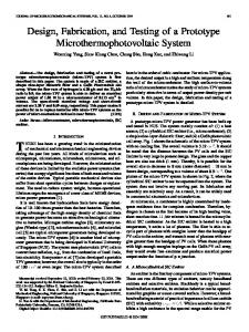
2. Electromechanical Design of LOCUS Sensing Device The purpose of this work is to develop a low cost ultrasonic (called LOCUS) that exhibits a fast processing time, a shorter minimum detection distance with a higher resolution in distance measurement for future deployment on the URVs. It has to be low cost to allow multiple sensor configurations and compact in physical dimensions. The overall structural design of LOCUS sensing device is shown in Fig. 1. The prototype LOCUS sensing device weight 2 kg and has an overall dimension of 190 mm (length) × 120 mm (width) ×60 mm (height) including the transducer’s support. By removing the buoyant float and other support during prototype testing, the dimensions of the proposed transducer size can be reduced to 100 mm (length) × 120 mm (width) ×20 mm (height). With the extendable transducer’s cable, it allows the transducer to be placed anywhere on URV platform. However, the current enclosure design of the proposed sensing device can only worked in shallow water of not more than 1m. Hence, an improved design to work in deeper water is needed in our future works.

Figure 1: Actual (left) and schematic diagram (right) of LOCUS transducer

2.1. Proposed Ultrasonic Sensor The LOCUS sensing device uses a short wavelength sound and a classic pulse echo detection method (similar to echo sounder system) for close-range measurement (maximum 2m) and obstacle avoidance (maximum 5m). The basic echo sounding system operates at a frequency range from 20 to 500 kHz. The 200LM450 transducer and signal processing module (see Fig. 2) consists of few main components such as amplifer, bandpass filter, microprocessor, transmitter (T) and a receiver (R) or transceiver with T/R switch.

The frequency of the ultrasonic sensor is chosen based upon the propagation range, beam spread and directivity. As a lower frequency is suitable for long range propagation, it results in less directivity (for a given diameter of the transceiver with the wider beam spread). Hence, it is more suitable to

4

choose a higher frequency. For short range measurement and obstacle avoidance tasks on URVs, the maximum detection distance of 5m is considered. There are many ultrasonic sensors available in market. In this project, a common ultrasonic sensor (see Fig. 2) such as 200LM450 is used. The sensor operates at 200kHz with bandwidth of 25kHz. It has 160dB (minimum) transmitting sound pressure and -180dB (minimum) receiving sensitivity with a total of 20 degrees beam angle. The resulting sound pressure level (SPL) at 5m is calculated to be 151dB after considering the loss due to wave absorption and SPL reduction at 5m. The voltage generated under this condition is approximately 35mV after considering the receiving sensitivity (voltage/Pa).

Figure 2. Physical appearance of 200LM450 transducer and signal processing module

2.2. Electrical System Layout The main feature of LOCUS sensing device is the single transducer system using the 200LM450 transducer, a self-calibration mode for operating in a different fluid medium, a customized module for signal amplification, and a noise filter (integrated with PW0268 chip) and a PIC-based microprocessor for signal control to achieve the desired data processing speed and distance resolution. In the self-calibration feature, it is used to eliminate the problem of measurement errors in different fluid medium such as fresh and sea water. It removes an additional sensor for detecting different fluid mediums. This mode can be activated by placing an object manually at a pre-fixed distance.

A 200LM450 transducer module with a signal-processing module is shown in Fig. 2. A fixed gain pre-amplifier and time controlled variable gain amplifier to amplify and vary the sensitivity of the receiving echo were also implemented. To eliminate the noise (known as ringing effect) from the receiving echo, a lower and upper band pass filter was incorporated. As shown in Fig. 3, the ringing effect on the echo is reduced by a signal-processing circuit consisting of a band pass filter.

Figure 3: Difference of responses without band pass filter (left) and with band pass filter (right)

5

The LOCUS sensing device starts the distance measurement by clicking a start button as shown in Fig. 4. The self-calibration mode is then activated using a calibration toggle switch. Since the basic echo sounding system works when the transceiver generates high-voltage electrical pulses and sends the signal to the transmitter, the transmitter converts these pulses into sound waves. The sound waves propagate through the fluid medium until it reaches target object’s surface and propagate back to the source. The receiver converts the echo into electrical pulses before amplification and filtering as shown in Fig. 2. A comparator uses the general-purpose amplifier, NPN 2N4401 to convert the analogue signal of the returning echo to a digital signal via a microprocessor, PIC18F4550.

After the sensor calibration, the fluid medium mode switch can be activated. As shown in Fig. 4, the control algorithm (using C programming language coding) is implemented in MPLAB environment to interface the microprocessor to the user’s computer (with MPLAB software installed for C programming) via a PICkit2 debugger/programmer. The other side of the programmer is connected to the microprocessor through an in-circuit serial programming (ICSP) that uses two input/output pins. A PICKIT2 programmer was used to enable the written C language to be downloaded into the microprocessor.

Figure 4: Schematic diagram of the components integrated in LOCUS

2.3. Program Flow Chart The following describes how the microprocessor determines the distance from the target object in underwater. It captures the falling edge of signal (as seen in Fig. 5) to a correct echo after the signal was amplified and filtered. The microprocessor transmits a 5V pulse of 0.1ms pulse duration to excite the 200LM450 transducer. The microprocessor has two 16-bit CCP (capture, compare, and PWM, module) to assist with measurement. This module allows the system to compute the number of the

6

count period between the transmitting and ringing pulse, and the receiving echo. When there is no ultrasonic pulse, the CCP1 module is held at “high." Once the transducer transmits the pulses, the timer in microprocessor starts the counting process, and the CCP1 module function record this initial value. The echo signal entering the CCP1 module holds at “low” until the end of ringing. The counting continues to count until the arrival of the echo signal. This arrival of echo signal goes low and causes the timer to stop counting and the CCP1 module function will register the final value. The number of counts is the difference between the final and the initial value as shown in Fig. 5.

Figure 5: Capturing the signal falling edges. The PIC18F4550 microprocessor is used to determine the number of counts between falling edges. The total time delay required can be achieved by using the correct number of instruction cycles in the C program. For example, the number of instruction cycle, nI (using 0.2µs per instruction cycle) is calculated to be approximately 5000.

nI 

Total time delay Time per instruction cycle

1  10 3 0.2  10 6  5000 instruction cycles 

(1)

To measure a distance up to 5m, twenty burst of 200kHz ultrasonic waves are required to produce an amplitude of 5V square signals to excite the 200LM450 transducer. The pulse time duration (t p ) is computed approximately 0.1ms as shown.

1  number of bursts frequency of square waves 1   20 0.2  10 6  0.1ms

tp 

7

(2)

Assuming the speed of sound (SOS ) is 1500m/s, each count defines the measurement resolution. As the timer for CCP1 is 16-bit, it has a maximum value of 65535 counts before it resets back to 0 and continues counting. As the number of trips (to and from the object) is equal to 2, the distance resolution (d R ) and the maximum distance ( M R ) can be calculated as follows:

d R  TOC  SOS  0.2 106 1500  0.3mm

TOC  Maximum counts  SOS NOT 0.2  10 6   65536  1500 2  9.83m

(3)

MR 

(4)

where T OC is the time per count, and NOT is the number of trips.

This calculated range is acceptable as the operating distance is within 5 m. From the computation, the device is capable of measuring an object up to a resolution of 0.3mm while minimizing the ringing effect. The application of a classical signal analysis technique in mechanical measurement called three-time majority method [21] is included into the correlation calculation to reduce the measurement error on the transmission before reverberations or secondary echoes are dissipated. To circumvent that, the period between each transmission cycle (n ) had been tested and showed to give a delay of 30 ms during the experimental test. As seen in Fig. 5, the transducer transmits one pulse, receive echo and hold the signal for 30 ms before the next measurements. The distance of the object (Ds ) was determined by averaging the three collected measurements as shown below.

Ds 

(TOC  NOC ) n1  (TOC  NOC ) n  2  (TOC  NOC ) n3  SOS  100 3  NOT

8

(5)

where NOC is the number of counts and ’3 ’ indicated the number of measurements.

2.4. Mechanical Design LOCUS sensing device was designed to measure the underwater objects while floating on the water. It must be able to float with good stability while measuring underwater object. By adjusting the length of the transducer cable, the sensor can be used to detect the depth of the target object. The electronics and switches were housed in a waterproofed casing shown in Fig. 6. Figure 6. Operating panel of LOCUS sensing device (front view)

LOCUS sensing device consists of three main components:

a top casing, bottom casing and

Styrofoam board as observed in Fig. 7. The top casing contains the electrical components while the bottom casing contains the transducer’s cable. The partition eliminates the water ingress; the fixer positions the two casings equally onto the Styrofoam board. The bracket is used to hold the three main components together during the test. With the opening of the transducer’s support unit being sealed by a cable gland, drilling of a hole is required. The float and bottom circuit casing were built and assembled. The drilled holes were sealed with waterproof silicon glue with cable glands. Figure 7: LOCUS sensing device layout Since the prototype is floating in the water, the initial and static transverse stability needs to be taken into consideration. All the objects must be symmetrical along its transverse axis to perform the calculation. This was done by adding an addition weight inside the cable casing. The additional weight decreases the vertical distance from K to center of gravity (KG) along the transverse axis. This increases the vertical distance from G to MT (GMT) and resulted in a huge increase in the stability of the prototype. The additional weight also minimizes the water ingress through the top electronic casing. A pictorial diagram for the stability calculation is shown in Fig. 8. Figure 8: Necessary stability for the ICON sensor prototype.

9

The additional weight is required to stabilize the device in water. With the original weight

Woriginal  1.313kg , density of water   1000kg/m3 and underwater volume of prototype V p  0 .0021 m 3 , the required displacement is VR  V p . The required additional weight is approximately 0.76kg .The placement of the additional weight is properly positioned to align with LCG and LCB at the same axis such that the transducer faces the underwater objects. The position of the additional weight was calculated using first principle of moment. The prototype is considered to be stable if the GMT is greater than zero. The vertical distance from B to the transverse metacentre (BMT) is 0.0517m and vertical distance from K to center of buoyancy (KB) is 0.0367m. Since the GMT is approximately 0.0371 (greater than zero), it implies that the stability of the prototype is acceptable.

3. LOCUS Sensing Device Simulation using LabVIEW LabVIEW (Laboratory Virtual Instrument Engineering Workbench) [22] developed by National Instrument, is a graphical programming environment suited for system-level design. LabVIEW was used to simulate the LOCUS sensing device. Figure 9 depicts the front panel of the LabVIEW based LOCUS sensing device system. The front panel allows the user to insert distance apart, operating fluid medium, and temperature, depth of the sensor, salinity level and transducer’s frequency. It also displays the outputs such as waveform graphs, time of flight (TOF), speed of sound (SOS) and error in measurement as compared to the experimental results.

This simulation was programmed and grouped into five parts as shown in Fig. 9. It includes the necessary settings of the transducer (e.g. distance apart from object and frequency of the sound wave), the fluid medium parameters and characteristics of actual pulse, the selection of operation device, the results of system information and the measurements. The pulse-echo method animation shows how the distance measurement device is able to correlate distance with sound waves. The speed of the animation can be adjusted using a control knob as shown.

10

Figure 9: Overview of LabVIEW based simulation of ICON sensor Part 1 (see Fig. 9): The boundary limits of width and depth are constrained by the beam width. The values on the boundary are presented in distance X of the transducer. Ultrasonic beam converges in the near-field region while diverging in the far-field regions. The beam boundary defines the limits of the beam at the point where it falls to a threshold value. To determine the beam spread angle from ultrasonic wave (emitted from the transducer), the following equation is used.

  sin 1

K D

(6)

With the wavelength of the ultrasonic waves written as:   V / F , equation (6) becomes:

  sin 1

KV DF

where F is the frequency of ultrasonic wave in Hz, V is the velocity of ultrasonic waves

(7) in m/s, D is

the diameter of the transducer in m and K is a constant dependent upon the beam boundary. The method to determine the beam spread and the shape of the transducer can be seen in Table 1.

Table 1. Constant value of circular shape transducer [23] Part 2 (see Fig. 9): The location where the device is operating, affects the accuracy of the measurement. Therefore, the system needs to identify the fluid medium characterized by the temperature, salinity and depth of the water in order to determine the actual speed of sound. However, using additional sensor increases the cost to the system. Hence, we assumed the speed of sound. Table 2 shows the realistic assumption, and the speed of sound obtained from the simulation as compared to the experimental results (in the next section).

Table 2: Parameters for different fluid medium- sea and fresh water

11

Part 3 (see Fig. 9): After the parameters and the fluid medium were determined, the time of flight (TOF) of the actual sound wave is computed using the following relationship.

Actual TOF 

Distance between transducer and target object 2 Actual speed of sound wave

(8)

Part 4 (see Fig. 9): The speed of sound is an important parameter to determine the TOF in (8). The speed of underwater sound (SOS) is a function of three variables (salinity, temperature and pressure). There are many empirical formulas to obtain this parameter. One of the common accepted methods [24] is shown below.

SOS  1449.08  4.57e  0.1522 Pe

 T  T 2       86.9  360  

 T  S  35     1200   400     

 1.33( S  35)e



T 120

(9)

 T S  35     2  20 10 

 1.46  10 5 P e

where T is the temperature in ˚C , S is the salinity in ppt and P is the pressure in N/m2. The LabVIEW based software using the parameters obtained from (8) and (9). By tuning the speed of sound or wave length, the TOF could be changed.

Part 5 (see Fig. 9): The digital echo signal output with an assumed width of the echo is used to simulate the signal to capture the lower edge of an incoming signal. The system will output the measured distance, the number of pulses transmitted and the speed of pulse waves at selected fluid medium mode. The measurement validity will reflect the minimum reading caused by the ringing effect. To determine the error in measurement, the difference between the actual distance measurements is displayed on the front panel. The percentage of measurement error is then calculated. When the fluid medium mode switch is activated (deactivated), the mode is set in the freshwater mode with sound speed equals to 1504 m/s (1544 m/s). The control pulse duration simulates the number of pulses transmitted and the ringing effects.

12

4. Experimental Tests in Water Testing and verification of the circuit and program is necessary to ensure that the real time measurement work as planned during the design and simulation stage. All the problems involving interfacing of components, programming errors, measurement capability are to be resolved during the experiment. The entire circuit boards of the LOCUS sensing device are connected as shown in Fig. 10.

Figure 10: Circuit layout of LOCUS prototype. The aims of this lab experiment (see Fig. 11) are to calibrate the integrated circuit in the water tank (0.60m long × 0.80m wide × 0. 20m high) and test the underwater distance measurement. In the experiment, the fresh water has a depth of 0.10 m at a temperature of 28oC. This primary experiment test ensures that all the electronics were interfaced correctly.

Figure 11: Calibration of LOCUS prototype in water tank The object is placed at a 0.50m apart from the transducer. The digital oscilloscope was used to display the output of microprocessor. Figure 12 (on the left) shows that the microprocessor sent a 5V signal at a 0.1ms period. As observed in Fig.13, the signal falls to 0V at the receiver side. The signal goes back to 5V when the echo was detected. This indicates that correct signal had sent through the CCP1 port in the microprocessor.

Figure 12: Sent pulse signal from microprocessor (left) and output digital echo signal to CCP1(right)

The system device is tested several times on the object placed 0.5m apart from the transducer. The microprocessor successfully displayed the measurement on the LCD. It could measure an average of 0.50m with a standard deviation of 0.004m and a root mean squared error of 0.017. The second

13

experiment (see Fig. 13) was conducted in a towing tank with a dimension of 15m×2.15m×1m. The test was conducted to analyse the measurement data in different fluid medium and target objects.

The object used in this experiment testing was an acrylic board and galvanized steel. Both the dimensions of the objects are 0.35 m × 0.24 m × 0.002 m. The PVC pipe in Fig. 14 was used to align the transducer and objects in the towing tank.

The object and transducer were placed on the

horizontal supports along the edge of the towing tank. The experimental setup is used to perform the measurement (in the left-hand side of Fig. 15) and the collect experimental data.

Figure 13: Overview of towing tank experimental setup for ICON sensor prototype Figure 14: Aligning target object and 200LM450 transducer for testing The end of the horizontal support both transducer and object was placed at 0.0575 m from the extreme side of the towing tank. Vertical supports were adjusted to align the midpoint of the object and transducer (as indicated by a yellow dotted line in Fig. 14) at different depth measurement. The actual distance between the transducer and objects was indicated on the side of the towing tank. The experiment consists of four tests. The temperature of the fresh water in the towing tank was at 25.5◦C . The depth of the transducer was 0.50 m, 0.17m, 0.12m and 0.12m for all test 1, 2, 3 and 4, respectively. The object used in test 1 to 3 was an acrylic sheet while the galvanized steel piece was used in test 4. The distance measured by the test circuit ranges from 0.40m to 5m (with an increment of 0.20m). Several measurement readings were collected. The mean, standard deviation and root mean squared error (RMSE) were determined. As seen in Fig. 15, it is apparent that the simulation result matches the actual distance. The sensor can measure a close distance of 0. 4m. These results show that the simulation model is able to measure the objects in freshwater accurately. However, there exists a small different due to the transducer that tilted slightly after the transducer horizontal support was changed.

14

Figure 15: Comparison of experimental and simulated results for test 1(0.5m depth), test 2(0.17m depth) and test 3(0.12m depth) From the experimental results in Fig. 16, it indicates that there are some differences between the freshwater and seawater mode. As compared to the simulated results, they exhibit the same trend with slight drifted as the measured distance increases. Table 3 shows the freshwater mode has errors less than 2.64% (that is less than the common trend of errors of more than 2.75% [25] when compared to the sea water). The RMSE is quite high in the sea water as compared to fresh water but its standard deviation is smaller in fresh water. This implies that the average magnitude of the error in sea water is higher. These phenomena is caused by the presence of many in homogeneities, including bubble layers close to the surface, living organisms, and mineral particles in suspension in sea water. The speed of sound can be quite sensitive in distance measurement under different fluid medium and depth due to salinity differences. Hence, the solution is to use the self-calibration modes in the program to obtain a better speed of sound in various fluid medium.

Table 3: Experimental value of fresh water and sea water underwater distance measurement Figure 16: Comparison of experimental and simulated results for fresh water and sea water From Table 3, it can be observed that different materials used for object distance measurement affects the distance measurement. As seen in the standard deviation, the target object material has more impact in sea water than fresh water at the depth of 0.12m. As seen in the relative percent difference between the acrylic and metal (as compared to the acrylic), the acrylic has a wider spread in the measurements and RMSE as compared to the metal object. The differences are contributed by the surface roughness of the material that causes different scattering of acoustic waves. In Table 4, the average magnitude of the error increases as the measured distance increases. The computed errors are less dominated in fresh water as compared to seawater. However, the two materials are able to reflect the transmitted ultrasonic wave to the receiver and can detect both metals and acrylic in underwater.

15

Table 4: Experimental value of different materials for underwater distance measurement During the pool experiment (see Fig. 17), the object used for this experiment was the wall of the swimming pool facing the LOCUS sensing device. The temperature of the pool water was at 28◦C. The device successfully floated in the pool without any supports (see Fig. 17). The device was also able to obtain several measurement distances that were similar to the actual distance from the walls.

Figure 17: Pool experiment for LOCUS sensor The device could take some disturbances caused by hand creating some wave on the surface. However, the device was unable to produce measurement with the aggressive wave generation due to excessive presence of bubbles. As seen in Fig. 18, there is approximately 12 percent error due to the effect of the waves on the LOCUS sensing device. The possible reason would be the disruption of sound wave transmission when massive bubbles were formed. As stated in reference [26] , the presence of air bubbles changes the density and compressibility of the fluid, affecting its speed of sound and resulting direction of the initial sound beam. This indicates that application of acoustic in high concentrations of bubbles, e.g. in the wakes of ships, at shallow depths when waves are breaking at the surface need to be avoided when performing the measurement. However, as the depth increases, these errors will decrease with less wave effect. Hence it is more viable to use this sensor in deeper water. In summary, the pool test results were quite successful and the data collected reflected that the LOCUS sensing device could measure the distance of an underwater target. Figure 18: Experiment results with and without wave during measurement in pool

5. Conclusion The development and testing of a low cost ultrasonic (LOCUS) sensing device was shown. The LOCUS sensing device uses the pulse echo detection method to reduce the detection capability. The device was tested at distances up to 5m in different fluid medium and target objects. The experimental results shown that the percentage difference for the seawater and freshwater measurement was reasonable as compared to the literature. When simulated in the ultrasonic distance measurement

16

software using LabVIEW, the simulated results show a reasonable agreement with the experimental results. In summary, the LOCUS sensing device was effective for close-range underwater distance measurement study. It provides a test-bed and simulation model for feasibility study of a typical ultrasonic sensor in underwater sensing application before actual implementation.

In the future works, the proposed low cost underwater distance measurement system will be implemented on an actual URV platform. Communication between multiple sensors will be explored using the same platform. The current enclosure design of the proposed sensing device can be improved by designing a new enclosure for deep water testing.

6. Acknowledgment This work was made possible by support of Newcastle University. The authors appreciate the valuable technical support of the academic and technical staff throughout the project.

7. References [1] Arshad M R (2009) Recent advancement in sensor technology for underwater applications, Indian Journal of Marine Sciences. 38(3): 267-273. [2] Snyder J (2010) Doppler Velocity Log navigation for observation-class ROVs, 2010 OCEANS: 1-9. [3] Arshad M R, Lucas J (1998) Underwater optical ranging system for ROVs. OCEANS '98 Conference Proceedings, 2: 1189-1193. [4] Nolan S, Toal D (2008) A low directivity ultrasonic sensor for collision avoidance and station keeping on inspection-class AUVs, Journal of Marine Engineering and Technology, A11: 1-11. [5] Yoon S H, Qiao C (2011) Cooperative search and survey using autonomous underwater vehicles (AUVs), IEEE Transactions on Parallel and Distributed Systems, 22(3): 364-379.

17

[6] Ribas D, Palomeras N, Ridao P, Carreras M, Mallios A (2012) Girona 500 AUV: From Survey to Intervention, IEEE/ASME Transactions on Mechatronics, 17(1): 46-53. [7] Zhang Y, McEwen R S, Ryan J P, Bellingham J G (2010). Design and tests of an adaptive triggering method for capturing peak samples in a thin phytoplankton layer by an autonomous underwater vehicle , IEEE Journal of Oceanic Engineering, 35(4):785-796. [8] Foote K G, Patel R, Tenningen E (2010). Target-tracking in a parametric sonar beam with applications to calibration, 2010 OCEANS:1-7. [9] Kocak D. M., Dalgleish F. R., Caimi F. M., Schechner Y. Y.. A focus on recent developments and trends in underwater imaging, Marine Technology Society Journal, 42, 1 (2008) 52-67. [10] Caimi F M, Kocak D M, Dalgleish F, Watson J (2010) Underwater imaging and optics: recent advances, IEEE Oceanic Engineering Society Newsletter: 21-29. [11] Liu J J, Jakas A, Obaidi A, Liu Y H (2010) Practical issues and development of underwater 3D laser scanners, IEEE Conference on Emerging Technologies and Factory Automation (ETFA) :1-8. [12] Wang C C, Tang D (2009). Seafloor roughness measured by a laser line scanner and a conductivity probe, IEEE Journal of Oceanic Engineering, 34(4):459 – 465. [13] Hwang P A (2012). Foam and roughness effects on passive microwave remote sensing of the ocean, IEEE Transactions on Geoscience and Remote Sensing, 50(8):2978-2985. [14] Simpson J (2008) A 1 Mbps underwater communications system using LEDs and photodiodes with signal processing capability, Master of Science thesis, North Carolina State University. [15] Wang JJ, Yuan D and Cai P (2010). Range resolution of ultrasonic distance measurement using single bit cross correlation for robots. 2010 IEEE International Conference on Information and Automation (ICIA): 917 – 923.

18

[16] Hirata S, Kurosawa MK and Katagiri T (2009). Real-time ultrasonic distance measurements for autonomous mobile robots using cross correlation by single-bit signal processing. IEEE International Conference on Robotics and Automation: 3601 - 3606 [17] Talebhaghighi Z,

Bazzazi F and Sadr A (2010). Design and simulation of ultrasonic denoising

algorithm using wavelet transform and ICA. 2010 The 2nd International Conference on Computer and Automation Engineering (ICCAE), 1: 739 – 743. [18] Johansson J and Martinsson PE (2001). Incorporation of diffraction effects in simulations of ultrasonic systems using PSpice models. 2001 IEEE Ultrasonics Symposium, 1: 405 – 410. [19] Jiang SB,

Yang CM, Huang RS, Fang CY and Yeh TL (2011) . An Innovative Ultrasonic

Time-of-Flight Measurement Method Using Peak Time Sequences of Different Frequencies: Part I . IEEE Transactions on Instrumentation and Measurement, 60(3): 735 – 744. [20] Zhang SY (2010). Research of Ultrasonic Distance Measurement Device. 6th International Conference on Wireless Communications Networking and Mobile Computing (WiCOM), 1-3. [21] Littlestone N, Warmuth M K (1989) The weighted majority algorithm, In Proceedings of 30th Annual IEEE Symposium on the Foundations of Computer Science, New York :256-261. [22] Hammad A, Hafez A, Elewa M T (2007) A LabVIEW based experimental platform for ultrasonic range measurements, DSP Journal, 6(2): 1-8. [23] Subramanian C V (2006) Practical Ultrasonics. Alpha Science International Ltd, Oxford, UK. [24] Grosso V A D (1974) New equation for the speed of sound in natural waters (with comparisons to other equations), J. Acoust. Soc. Am, 56(4):1084-1091 [25] Seawater Farming. Retrieved September 1723, 2012, from Mission 2014: Feeding the World: http://12.000.scripts.mit.edu/mission2014/solutions/seawater-farming. [26] Kinsler L E, Frey A R, Coppens A B, Sanders V (2000) J. Fundamentals of acoustics, John Wiley & Sons Inc, USA.

19

List of Figures

Figure 1: Actual (left) and schematic diagram (right) of LOCUS transducer

Figure 2. Physical appearance of 200LM450 transducer and signal processing module

20

Figure 3: Difference of responses without band pass filter (left) and with band pass filter (right).

Figure 4: Schematic diagram of the components in ICON sensor

Figure 5: Capturing the signal falling edges.

21

Figure 6. Operating panel of LOCUS sensing device (front view)

Figure 7: LOCUS sensing device layout

Figure 8: Necessary stability for the ICON sensor prototype.

22

Part 1  Part 4

Part 2  Part 5

Part 3 Figure 9: Overview of LabVIEW based simulation of ICON sensor

Figure 10: Circuit layout of LOCUS prototype.

Figure 11: Calibration of LOCUS prototype in water tank

23

Figure 12: Sent pulse signal from microcontroller (left) and output digital echo signal to CCP1(right)

Figure 13: Overview of towing tank experimental setup for ICON sensor prototype

Figure 14: Aligning target object and 200LM450 transducer for testing

24

Figure 15: Comparison of experimental and simulated results for test 1(0.5m depth), test 2(0.17m depth) and test 3(0.12m depth)

Figure 16: Comparison of experimental and simulated results for fresh water and sea water

25

Figure 17: Pool experiment for LOCUS sensor

Figure 18: Experiment results with and without wave during measurement in pool

26

List of tables Edge (%dB)

K Through transmission technique 1.08 0.54

10 50

Pulse echo techniques 0.87 0.51

Table 1. Constant value of circular shape transducer [20] Singapore Freshwater seawater 29.5 28 35 0 Assume to be negligible

Parameters

Temperature [˚C] Salinity [ppt] Pressure [N/m2] Speed of sound 1544.48 1504.4 (from simulation) [m/s] Table 2: Parameters for different fluid medium- sea and fresh water Average Readings    Operating Condition 

Standard  Deviation (in cm) 

Root Mean  Squared Error  (in cm)  Fresh  Sea  Water  Water 

Water  Depth 

Target  Object 

Fresh  Water 

Sea  Water 

0.50m 

Acrylic 

0.56 

0.17 

4.16 

0.17m 

Acrylic 

0.48 

0.69 

3.72 

0.12m 

Acrylic 

1.68 

0.75 

0.12m 

Galvanized  Steel 

1.00 

0.60 

Percentage Error (in %)  Fresh  Water 

Sea  Water 

Difference  (FW‐SW) 

14.58 

1.09 

3.46 

2.37 

17.24 

0.65 

2.95 

2.30 

8.96 

25.72 

1.40 

3.80 

2.40 

5.24 

24.44 

0.78 

3.42 

2.64 

Table 3: Experimental value of fresh water and sea water underwater distance measurement Depth (in m)

0.12m

Average Readings (in cm) Standard Deviation (Fresh Water) A M Rel. % Diff

Standard Deviation (Sea Water) A M Rel. % Diff

Root-Mean-Square Error (Fresh Water) A M Rel. % Diff

1.68

0.76

8.96

1.01

77.15

0.61

98.45

5.24

55.89

Root-Mean-Square Error (Sea Water) A M Rel. % Diff 25.73 24.45 29.36

Table 4: Experimental value of different materials for underwater distance measurement  

27