When doing this, we must free the new position h of the accessed item by pushing ...... Ptk+1- tk. (e,h y-1(A)) = Ptk+1- tk. (y,A). Conversely if there exists a group ...
1
State-transitive Markov processes, random walks on groups, and self-organizing data structures
Philippe Chassaing1
Suggested running head : Self-organizing data structures and random walks.
1Département de Mathématiques, Université de Nancy 1, B.P.239, 54506 Vandœuvre Cedex, FRANCE
Telephone number : 83.91.21.10 Fax number : 83.28.09.89
2 State-transitive Markov processes, random walks on groups, and self-organizing data structures
Philippe Chassaing
A BSTRACT. We prove the optimality of the move-to-front rule in the class of on-line selforganizing sequential search heuristics for data structures, taking advantage of the fact that the sequence of requested items is a Markov chain F whose symmetry group G F acts transitively on the set S of items (F is then said to be state-transitive ). We state corresponding general results on controlled Markov chains with non trivial symmetry group. In order to have a better knowledge of state-transitive Markov processes, we give a construction of any state-transitive Markov process F with the help of a random walk on its symmetry group G F , and a characterization of state-transitive Markov processes F such that their state space S can be endowed with a group structure implying F is a random walk on the group S.
Key words : Markov process, random walk, self-organizing data structure, controlled Markov chain, decision rule.
3 1. INTRODUCTION . In this work, we consider a homogeneous Markov process X = (X t ) t∈ T on
(Ω,a,(Px)x∈S,(f t)t∈T), with state space (S,a’), time set T and transition semigroup (Pt)t∈T ; we shall take T =
N or R+. We call any mapping from S to S which is one to
one, onto and bimeasurable, a permutation of S . Let φ be a permutation of S and let Xφ be the Markov process defined by : Xtφ = φ(Xt). Then we have, from Dynkin (1) : Definition 1. A permutation φ of S is a symmetry of X if one of the equivalent conditions is satisfied :
a
i) ∀x∈S, ∀A∈ ’, ∀t∈T
Pt(x,A) = Pt(φ(x),φ(A)),
ii) for any t in T, and any real bounded measurable function f on S, (Ptf)oφ = Pt(foφ),
iii) for any state x, Xφ has the same law under
Px than X under Pφ(x).
Definition 2. If the action of GX on S is transitive, the Markov process X is said to be state-transitive, as well as its semigroup. If GX contains G as a subgroup, then X, or its semigroup, are said to be G-symmetric. The state-transitive terminology is taken from algebraic graph theory. When X is statetransitive, there is only one orbit in S under the action of G X, so each state plays the same rôle with respect to X. For instance, when S is finite and T =
N, a sequence X of i.i.d.
random variables is state-transitive if and only if the X t, t > 0, are uniformly distributed on S, and more generally, state-transitivity of a Markov chain X entails that the uniform law on S is invariant for the semigroup of X. In section 2 , we describe a problem of stochastic control of a Markov chain X, with applications in computer science, which has motivated our investigation of the above questions : the state Xn+1 of a system at time n+1, is given by an expression of the form X n+1 = f(Fn,X n,A n),
4 where An is the control taken at time n, and Fn is an auxiliary stochastic process. Due to the special form of f, it turns out that, if we let (F n)n≥0 be a state-transitive Markov process, it allows a state space reduction for X , so we can sometimes find a policy An = R(Xn) whose long run average cost is optimal. In section 3, we give general formulations of the results proved in section 2, concerning controlled Markov chains with non trivial symmetry group, or, more generally, lumpable controlled Markov chains. The two last sections are devoted to an exploration of the notion of state-transitive Markov process. In section 4, we characterize Markov processes whose state space S can be endowed with a group structure making of them a random walk on the group S. It allows us to find the appropriate group structure when it exists, as in example 3, or to show that it does not exist, as in example 2. Note that the proofs of theorem 4 or 5 in section 4 are very simple, once their statements are given, but we did not find these properties stated elsewhere — they were announced in Chassaing (2) —, though they give an answer to a question in Diaconis (3), p.20, for instance. Let us mention, however, that section 4 of Glover
(4)
seems to deal with the same kind of problems, though not very
explicitly, and concerning the very special case of transient Borel right processes. In section 5 we give a general construction of any state transitive Markov process X, using an adequate random walk on its group of symmetries.
2. SELF ORGANIZING SEQUENTIAL SEARCH DATA STRUCTURES. Let us describe a simple example of a self-organizing sequential search data structure. Let S = {1,2, ... ,M} be a set of items ; assume that these items are stored in places, and that the set
p of places is {1,2, ... ,M}. When an item is requested, it is searched for in
place 1, then, if not found, in place 2, and so on, and a cost p is incurred if the item is finally found in place p. Once the item has been found, a control is taken on the search process by replacing the item in a wisely chosen place : for instance, closer to place 1, in
5 such a way that the most frequently accessed items spend most of their time near place 1. When doing this, we must free the new position h of the accessed item by pushing the items remaining between the old position k and the new position h, the non-accessed items retaining their relative order, as in figure 1. Let F = (F n)n≥1 be the sequence of requested items ; we shall assume it is a Markov chain, with state space S and transition kernel P. Let Dn be the disposition of items in from S to
p at time n, i.e. the one-to-one mapping
p giving the position of each item just before the request and replacement of Fn
; D0 is the initial disposition ; lastly An is the control taken after request of F n, i.e. the place where Fn is replaced.
B B G H D Fn = B
G H D
Dn(Fn) = 6
Dn+1(Fn) = 3 = An Figure 1
Since we can write : Dn+1 = f(Dn,Fn,An)
(2.1)
for a suitably chosen mapping f, the stochastic process X = (X n ) n≥0 , where Xn =
6
(Dn,Fn), is a controlled Markov chain with finite state space S' = SM S and finite control set A =
p. Here, SM denotes the symmetric group of order M!.
The cost c(i,a) incurred when the system is in state i = (x,k) and when the control a is taken, is given by : c(i,a) = x(k), so the cost Cn incurred at time n is given by : Cn = Dn(Fn).
6 We recall briefly some basic facts from controlled Markov chain theory (for more information see Derman
(5)).
First the law of the stochastic process X depends on the
kernel (pi,j(a))(i,j,a)∈S’6 S’6 A, on the law of X0 and on the decision policy (or rule) used, where pi,j(a) denotes the conditional probability pi,j(a) =
P(Xn+1 = j / Xn = i, An = a and Hn ∈ B).
Hn is the history of the process up to time n, i.e. H n = (X0, A0, X1, A1, ... , An-1, Xn).
The fact that
P(Xn+1 = j / Xn = i, An = a and Hn ∈ B) depends on Hn only through Xn is
the Markov property for controlled Markov chains. For a self-organizing data structure, the Markov property follows readily from (2.1), and there is an expression of p i,j(a) in terms of the kernel P of F. An admissible rule R is a mapping from the set of histories to the space of probability measures on A, and one says that the policy R is used if, at each time n, the conditional law of An , given that Hn = h, is R(h). For the special case of self-organizing data structures, an admissible rule is called an "on-line self-organizing sequential search heuristic". In order to indicate the dependence of the probabilities on the rule and the starting state,
PR,i(E) will denote the probability of the event E when rule R is used and
the starting state is i. An important subclass of the class
c of admissible rules is the class cD of Markovian
stationary and deterministic policies, i.e. policies such that An = ψ(Xn) (the conditional law of An, given that Hn = h, is a point mass and depends on Hn only through Xn). These policies have two striking properties : first if R is in
cD then, under PR,i, X is a
homogeneous Markov chain, and beside of that, a result of Derman (5) states that among the optimal rules for the usual criterion (to be defined below), there is always a rule of
cD, i.e. the search for an optimal rule in c reduces to the search for an optimal rule in cD.
7 We shall retain a classical criterion for the evaluation of a rule R, the long run average cost, n
1 φR(i) = liminf n+1 ∑ n k=0
E R,i(c(Xn,R(Xn))),
and the rule R is said to be better than R’ if φR(i) is lower than φR’(i) for each starting state i. If R is in
cD, φR(i) is of course a true limit.
From now on, we shall thus consider only rules of
cD, and we shall not distinguish
between R and ψ, i.e. R will be a mapping from S’ to A. In the case of sequential data
cD which is of special interest, since the policies of this class are easy to implement and of low computational cost : it is the class cL of "library
structures, there is a subclass of
type" policies (see Letac (6) and Dies (7)). Definition 3. A rule R of mapping f from
c D is in c L if R(x,k) depends only on x(k) ; to each
p to A, is thus related a "library type" policy
Rf defined by Rf(x,k) =
f(x(k)). If we let fF (resp. fB, fT) be defined to be identically 1 (resp. identically M, resp. fT(1) = 1 and fT(k) = k-1 when k ≥ 2), then the associated policy RF (resp. RB, RT) is called a move-to-front rule (resp. move-to-back rule , transposition rule ). In table I we compare the evolution of the system with the same sequence F, but two different policies. When the Fn are i.i.d., it is known from Rivest (8) that RT has a lower average cost than RF, but simulations have shown that RF often performs better than RT (see Bentley and McGeoch
(9)).
According to the authors, this is due to the fact that in
practice F shows a "locality" phenomenon : the request of a given item at time n increases the probability for the same item to be requested at time n+1. For instance, it is clear in table I that move-to-front performs better than transpose, because item D is requested twice in a row. Thus the usual assumption of independence on the Fn has to be dropped, and it is more natural to assume F Markovian, with a kernel P such that pi,i is greater than pi,j, j ≠ i (note that in Lam et al. (10), the performance of RF and RT is computed explicitly for some kernels P such that RF performs better than R T). Furthermore, since in the
8 simulations of Bentley and McGeoch
(9)
RF appears to be optimal in some cases, and
very close to the best in most of the other simulations, a natural question is that of the existence of kernels P for F, such that RF is average cost optimal in the class
c. Some
state-transitive kernels happen to give an answer, but we need one more definition.
D0 =
(
move-to-front rule
transposition rule
A B C D
A B C D
1 2 3 4 1 2 3 4
);F =D;A =1;C =4 0
0
D0 =
0
(
D A B C D1 =
(
1 2 3 4 2 3 4 1
1
D1 =
1
(
D A B C D2 =
(
1 2 3 4 2 3 4 1
2
2
D2 =
(
A D B C D3 =
(
1 2 3 4 1 3 4 2
0
0
0
1 2 3 4 1 2 4 3
);F =D;A =2;C =3 1
1
1
A D B C
);F =A;A =1;C =2 2
);F =D;A =3;C =4
A B D C
);F =D;A =1;C =1 1
1 2 3 4 1 2 3 4
1 2 3 4 1 3 4 2
);F =A;A =1;C =1 2
2
2
A D B C
)
D3 =
(
1 2 3 4 1 3 4 2
)
Table I
Definition 4. Let SM act on S' as follows. When i = (x,k) is in S' let gi = (xog-1,gk). If G is a subgroup of S M and R is a map from S' to any other set, let us call R G symmetric if it is constant on the orbits of G on S'. Then we have :
9 Theorem 1. If P is G-symmetric, then among the average cost optimal policies of
cD, at least one is G-symmetric. The action of an element g of SM results from renumbering the items : if the original number of an item is k, let gk be its new number ; then the mapping associating to the new number of an item its place number is xog-1, where x is the mapping related to the original numbering. Since a library type policy is insensitive to the specific item which has been found, but depends only on the place where this item has been found, such a policy should be insensitive to a specific numbering, and it should choose the same action when the state of the system is (x,k) or (xog-1,gk). In other words, we should have : Proposition 1.
cL is the class of SM-symmetric policies of cD.
Besides, it is well known that : Proposition 2. Let J = [ai,j] (i,j)∈ S 6 S , with ai,j = 1 - δ i,j and let I be the identity matrix ; then
m = {α I+βJ / α ≥ 0, β ≥ 0, and α + (M-1)β = 1} is the class of SM-
symmetric transition kernels with state space S. Thus, if we want to find a kernel P such that RF is optimal, a first try could be with an element of
m, where we know that at least one library type policy is optimal. This try
gives : Proposition 3. If P is in
m , then RF is optimal in the class c if α ≥ β , RB is
optimal if α ≤ β, and the optimal average cost is 1/2(M+1- |αM - 1|). This result bears out the explanation of Bentley and McGeoch, since when α ≥ β, P is a natural modelling of the locality phenomenon they invoke. Note that, to my knowledge, no result of optimality of a policy in the class
c of
admissible policies has been obtained so far, though problems of this kind had been addressed by many computer scientists and probabilists : in the independant case, Kan
10 and Ross
(11)
obtain the optimality of the transpose rule in a subclass of
c L for a
particular distribution of items, and the optimality of the transpose rule in the same subclass of (12),
cL and for a general distribution of items is studied in Dies (7) and Kowalska
but for a very rough approximation of the long run average cost. In Bentley and
McGeoch
(9)
and Sleator and Tarjan (13), the long run average cost criterion is replaced
with some kind of worst case criterion. In the Markovian case, a beautiful expression of the average cost of RF in terms of P is given in Lam et al. (10), but optimality questions are considered only in Kapoor and Reingold (14), where improvements of the move-tofront rule, with respect to different criteria, are investigated. The optimality of RF in such a large class as
c has its price : the stochastic control
approach of self-organizing data structures involves checking the Bellman optimality condition for a given policy, and it requires to solve the linear system (2.2) below, with
6
rank M (M!), where the unknowns are the so-called "values" of each state, plus the average cost (we give a brief account of these matters below). An analogous problem such as computing the steady state probability or studying recurrence for the Markov chain D = (Dn)n≥0 is not easy even in the independent case (see references (15, ... ,18)), so choosing P in
m is a reasonable precaution for computations to be tractable. If we want
to check the Bellman optimality condition for RF with kernels P in a less restricted class than
m , the following theorem is of some help, allowing a reduction of the rank of
(2.2) : Theorem 2. If P is G-symmetric, then the value function associated with a Gsymmetric policy is itself G-symmetric. Before giving some applications of theorem 2, we recall briefly the Bellmann condition, which is only a sufficient condition for optimality of a rule R of
cD. First one defines the discounted cost of the rule R, ∑ αn ER,i(c(Xn,R(Xn))), 0 < α < 1.
is satisfied by at least one rule in ΨR(α,i) =
cD, but which
n≥0
11 It has the following expansion : 1 ΨR(α,i) = 1-α φR(i) + vR(i) + εR(α,i) with
lim εR(α,i) = 0,
α→1-
and vR(i) is called the value of the state i. We next give the usual form of Bellman's condition : Proposition 4. Let yR(i,a) := (yR1(i,a),yR2(i,a)) be defined by : y R1(i,a) := ∑ pi,j(a) φR(j) - φR(i) j∈ S'
y R2(i,a) := c(i,a) + ∑ pi,j(a) vR(j) - vR(i) - φR(i) j∈ S'
Let A(i) (resp.B(i), C(i)) be the set of actions a such that yR(i,a) is lexicographically lower than 0 (resp. 0, greater than 0), and note that yR (i,R(i)) is zero. Now R is said to obey the Bellman optimality condition — R is said Bellman-optimal — if A(i) is void for each i. This entails the optimality of R with respect to the long run average cost.
"
Proposition 5. If R’(i) belongs to A(i) B(i) for each i, then, for each i :
φR’(i) ≤ φR(i). If furthermore, there exists an i such that R’(i) belongs to A(i), then lim - ΨR(α) - ΨR’(α) > 0. α→1
Similar properties hold if we reverse inequalities, provided that A(i) is replaced with C(i). In order to check that the Bellman condition is satisfied, one has to compute the φR(i) and vR(i). When, under
PR, the Markov chain X has only one recurrent class, things are
greatly facilitated : in that case φR(i) does not depend on i and the set of solutions of the system vi + φ = c(i,R(i)) +
∑ pi,j(R(i)) vj,
i ∈ S’,
(2.2)
j∈S’
is
{(φR(i0),(vR(i) + K)i∈S’) / K ∈ R}.
It follows that in order to check the Bellman condition for R, one can use any solution of (2.2) indifferently instead of the true values of the φR(i) and vR(i).
12 Let us mention two applications of theorem 2 (for more details see Chassaing (19)) : - Let S be endowed with a cyclic group structure and let F be a nearest neighbor random walk on S (identified with
Z/MZ), with law µ = α δ0 + β δ1 + γ δ-1. Then P is
G-symmetric, where G is the cyclic group generated by the permutation τ := (1,2, ... ,M). From Theorem 2, we have that : vR(σ,k) = vR(σoτ-k,1). This allows to guess that vR(σ,1) is the number of inversions of σ, when γ is zero, and in the general case, that vR(i) takes the following form vR(σ,1) = ∑ α i,j 1≤ix(j).
After computation of the αi,j, it follows that RF satisfies the Bellman condition if and only if α ≥ (βM-1 + γΜ−1)(β - γ)/(βM-1 - γΜ−1). This last condition is fulfilled when α ≥ β∨γ, which would be the natural modelling of a locality phenomenon in this setting. - Let M = pq, pα + (q-1)pβ = 1 and let S be endowed with a group structure such that K 1 ,K2 , ... ,Kq are the right cosets of a subgroup K of order p of S. Let F be a left random walk on S, the law µ of which has the density α
`K + β `Kc with respect to the
counting measure. In other words, when an item of Ki is requested, the next item will be any of the items in Ki with probability α, or any of the items outside Ki with probability β. When α ≥ β, this gives a realistic model, as pictured in Knuth
(20)
p.399 : “small
groups of keys tend to occur in bunches” . The group G of symmetries of P is then a wreath product (see
(3))
of Sp and Sq, and G-symmetric functions f on S’ are just those
functions on S’ which depend on i = (x,m) only through ( x (m) ,x(K1 ), x(K2 ), ... , x(Kq)), with the following additional property : let K(m) be the Ki to which m belongs, then, x(m) and x(K(m)) being given, f is a symmetric function of (x(Ki))Ki≠K(m). This hint at the form of the vi, solutions of (2.2), suggests our guess that the value of the state
13 (x,m) is proportional to the center of gravity of x(K(m)). We deduce in reference (19) that RF is optimal when α ≥ β. Proof of Theorems 1 and 2. In these proofs only, we shall consider transition kernels other than P for the item process F, and thus several kernels for the controlled Markov chain X itself. Hence sometimes we must indicate the dependence of the law of X, not only on the rule R and the starting state i, but also on P : the values, long run average costs and amortized costs will be denoted by vR,P(i), φR,P(i) and ΨR,P(α,i). Let f be the mapping which, to (Dn,Fn,An), associates Dn+1. We have : f(Dnog-1,gFn,An) = Dn+1og-1. This is the result of the control An on the system, seen by an observer XX which would have numbered the items differently, i.e. an item we numbered k, would have been given by XX the number gk. Seen by XX, the system evolution is thus described by the process Y = (Yn)n≥0, with Yn = (Dnog-1,gFn). The item process gF = (gFn)n≥0 seen by XX does not have P as its kernel, but instead its transition kernel is gP = g*Pg*-1, where g* is the permutation matrix associated with g. If the policy R is used, XX believes that the policy really used is gR, defined by gR(i) = R(g-1i). Conversely, the cost Cn incurred at time n is the same for him as for us (D n(Fn) = Dnog-1(gFn)). We thus have :
and consequently :
Ψ R,P(α,i) = Ψ gR,gP(α,gi) φ R,P(i) = φ gR,gP(gi) . v R,P(i) = v gR,gP(gi)
This gives theorem 2 at once. From now on, we assume that R and P are G-symmetric, and thus that φR and vR are G-symmetric. We let g be an element of G, and we drop the subscript P in the notation. We have : pi,j(a) =
P(Xn+1 = j / Xn = i and An = a) = P(Yn+1 = gj / Yn = gi and An = a),
14 so it follows from the assumptions that : pi,j(a) = pgi,gj(a). The point is that A(i) is G-symmetric. We can thus run the policy improvement procedure (see Derman
(5))
with a slight change : we start from a policy R0 assumed to be G-
symmetric ; now either the A( i) are all empty and R0 is optimal, since it satisfies the Bellman optimality criterion, or there exists a state i 0 and an action a0 such that a0 ∈ A(i0), and in the latter case a0 ∈ A(gi0) for each g in G. Let R1 be defined by R1(i) = R0(i) unless i is in the orbit of i0 under the action of G, and in this last case let R1(i) = a0. Iterating this procedure, if no G-symmetric policy meets the Bellman optimality condition, we can construct an infinite sequence (Rn)n≥0 of G-symmetric policies. As in Derman (5) lemma 3 page 71, ΨRn+1 is then strictly less than ΨRn in the neighborhood of 1-, so no two policies of our sequence can be the same. This is impossible since there is only a finite number of G-symmetric rules, so some G-symmetric policy meets the Bellman condition.
#
Proof of propositions 1 and 2. That
m is the class of SM-symmetric transition kernels
is well known (see chapter V of Wielandt (21)) : when P is G-symmetric it means that (i,j)
6
→ pi,j is constant on the orbits of S S under the action of G, but since SM is 2-transitive, it has 2 orbits, the diagonal one and its complement. Now, for the SM-symmetric rules, if we let i = (x,k) and j = (y,m) be two elements of S', and g a permutation of S, we have j = gi if and only if : g = y-1ox and m = y-1ox(k), and this leads to :
y(m) = x(k),
but, reciprocally, it is obvious that if y(m) = x(k) then j = gi if and only if g = y-1ox. It follows that the class of S M -symmetric policies is exactly proposition.
c L , and we have the #
15 Proof of proposition 3. Let R = RF and let i = (x,k) be in S'. It is clear that for n ≥ 1, the average costs
ER,i(Cn) take the same value :
C* = α - β + M+1 Mβ. 2
Besides :
C0 = x(k)
a.s. with respect to
PR,i.
It follows at once that : λ ΨR(λ,(x,k)) = x(k) + 1-λ C*,
and thus :
φR(i) = C* and vR(i) = x(k) - C*.
We can now see whether R obeys the Bellman condition. Since, under y1R is identically zero, we only have to check that yR1 is positive, i.e. :
PR, X is ergodic,
x(k) ≤ x(k) - C* + (α - β) a + M+1 Mβ. 2 We get the optimality of RF , provided that α - β ≥ 0. If α - β ≤ 0, the same kind of computations show that RB is optimal and that its average cost is : C** = (α - β) M + M+1 Mβ. 2
#
There is a more general fact behind theorem 2 : let X be a G-symmetric Markov process, with kernel P, and let Π be the projection from S onto S/G, its quotient space under the action of G. Then we have : Proposition 6. Let Y = (Yn ) n ≥ 0 be defined by Yn = Π (X n ) : then Y is a Markov process. As usual when the quotient process is Markovian, the time τ that X spends in a given orbit A is either 0, +∞ or geometrically distributed with parameter P(x,A) (x ∈ A), and for each orbit A such that P(x,A) is positive, the evolution of X inside the orbit is governed by a kernel PA, which is proportional to the subkernel of P associated with A, with τ being independent of this evolution ; the only property specific to this particular quotient process is that each such PA is state-transitive. Proof. See Dynkin (1) for the essentials. #
16 Thus one could think of splitting the study of the process X into the study of the quotient process Y and that of the state-transitive processes on each orbit : this is another reason for focusing on state-transitive processes. Going back to our self-organizing data structures, from the fact that F is G-symmetric, and that, once a G-symmetric rule R has been selected, the Markov process X, as well as the cost function c(i,R(i)), are G-symmetric, it follows that the long run average costs and amortized costs can be studied through the quotient process Y = Π(X), thus allowing the reduction of the rank of system (2.2). Theorem 1 can also be derived from an extension of proposition 6 to controlled Markov chains, that we shall expose in the next section.
3. LUMPABLE CONTROLLED M ARKOV PROCESSES. Let us consider a controlled Markov chain with state space S, and action space A, both finite. Let (pi,j(a))i,j∈S,a∈A be its kernel and c(i,a) its cost function. Finally, let (E1,E2, ... ,Er ) be a partition of S, and let π be the projection from S to {1,2, ... ,r} := S/π, associated with this partition. Theorem 3. If for any fixed action a and any element k of S/π , the following functions : i→
∑
p i,j (a),
j∈Ek i → c(i,a),
and
factor through π (i.e. are constant on each Em), then among the decision rules that factor through π, at least one is optimal in
c.
Corollary 1. If the group G acts on the space S and if for any element (i,j,g,a) of
66 6
S S G A we have : pgi,gj(a) = pi,j(a) and c(i,a) = c(gi,a), then among the G-symmetric decision rules, at least one is optimal in
c.
17 Theorem 1 is of course a consequence of corollary 1. The following corollary found applications in Chassaing (19) : Corollary 2. Assume that the cost function c(i,a) does not depend on a. If for any fixed action a and any state j, the function i → pi,j(a) factors through π, then among the decision rules that factors through π, at least one is optimal in
c.
~ Proof of theorem 3. Consider a rule R = R o π. From the hypothesis we can define a function f on S/π as follows : f(π(i)) := c(i,R(i)). The stochastic process Yn := π(Xn) is a Markov process under
PR. It follows that
ER[c(Xn,R(Xn)) | X0 = i] = ER[f(Yn) | Y0 = π(i)], so ΨR(α,.) factors through π, and as a consequence, φR and vR too (set φR := ~ φ o π, vR = ~ v o π). Now, let ~ pπ(i),k(a) :=
∑
p i,j (a).
j∈Ek We have : y1R(i,a) = ~φ(π(i)) -
∑
∑ p i,j(a)) ~φ(k) = ~φ(π(i)) - ∑
k∈S/π j∈Ek
~pπ(i),k(a) ~φ(k).
k∈S/π
2 So y1R(i,a) factors through π. For the same reasons yR (i,a), A(i), B(i) and C(i) factor
through π. Now we can start the Howard algorithm with the initial rule R 0 = R. Either A(i) is void for each i, and R0 is optimal in
c, or there exists a state i0 and an action a0
such that a0 belongs to A(i0) (it follows that a0 belongs to A(i) for any i in Eπ(i0)). In the latter case, let R1 be defined by R1(i) = R0(i) unless i is in Eπ(i0), and in this last case let R1(i) = a0. The rule R1 factors through π, and from proposition 5 we deduce that
18 lim ΨR0(α) - ΨR1(α) > 0.
α→1-
The end of the proof is the same as in theorem 1.
#
Proof of corollary 1. Let π be the projection of S on the space of its orbits under the action of G. The hypothesis of theorem 5 are then clearly satisfied.
#
Proof of corollary 2. Here we cannot just apply theorem 3 since the hypothesis concerning the cost function is generally not satisfied. Let us introduce a new cost function c’(i,a), defined by c’(i,a) :=
∑ p i,j(a)
c(j).
j∈S Let C‘n be the cost incurred at step n for this new cost function. Of course we have : C‘n :=
ER,i[Cn+1 | Xn],
so the associated discounted cost Ψ‘R(α) is given by : Ψ R‘ (α,i) = 1/α(Ψ R(α,i) -
ER,i[C0]) = 1/α(ΨR(α,i) - c(i,R(i)))
It follows at once that : φ‘R(i) = φR(i), and that optimal rules are the same for the two costs.
#
We have even that : v‘R(i) = vR(i) + φR(i) - c(i,R(i)), so finally y‘R = yR, and rules satisfying Bellman condition with respect to c or to c’ are exactly the same rules.
4. ST A T E - TRANSITIVE M ARKOV PROCESSES AND RANDOM WALKS ON GROUPS.
19 The fact that there is more hope for the computations of optimal policies to be tractable when F is state-transitive gives us a motivation for proceeding to an exploration of statetransitive Markov processes. The first example of such processes is given by random walks on groups. We give below a necessary and sufficient condition on G X for the existence of a group structure on S such that the Markov process X is a random walk on the group S. In this section, unless otherwise stated, T is
N.
First, let us illustrate our purpose with some representative examples of state-transitive Markov processes. EXAMPLE 1. Let X be the standard Brownian motion on
Rd ; then GX is the group of
affine isometries. 12
α
1
β
2
α
45 34 25
14
35
8
3 β
β
7 23
α
13
15
4
24
Figure 2
6
β
α 5
Figure 3
EXAMPLE 2. Let X be the nearest neighbor random walk on the Petersen graph (see figure 2) : the vertices are the subsets with cardinality 2 of {1,2,3,4,5} and two vertices are neighbors if and only if they are non intersecting. The symmetry group of X is then
S5, the symmetric group with 5! elements. EXAMPLE 3. Let S be {1,2, ... ,2n}, n > 1, α and β be positive numbers such that α + β = 1, and X be the Markov chain on S with kernel P = [pi,j] defined by p2k,2k+1 =
20 p 2k+1,2k = α and p2k,2k-1 = p2k-1,2k = β, as in figure 3. Then GX is isomorphic to the dihedral group with 2n elements if α ≠ β, and with 4n elements otherwise. E XAMPLE 4. Let T =
N and X be a Markov process on Sd, the sphere of R d+1,
associated with a probability measure µ on [0,2] in the following way : the distance Yn+1 between Xn and Xn+1, is picked at random with law µ, and independent from
fn ; the
law of Xn+1, under the condition {Xn = x and Yn+1 = r}, is uniform on the intersection of Sd with the sphere whose center and radius are x and r respectively. Then G X contains O(d) as a subgroup. Definition 5. The permutation group H is said to be regular if for any couple (x,y)
6
in S S, there is a unique element φ in H such that y = φ(x). This terminology is taken from Wielandt
(21) ,
for instance. According to Jordan
(1870), when H is a regular permutation group of S, S can be endowed with a group structure such that H is the group of right translations with respect to this group structure. This is done as follows : let e be given in S ; we know, from the definition of a regular group, that there exists only one element hx in H such that hx(e) = x, so that the mapping
h(h) = h(e), from H to S, is one-to-one and onto, with h-1(x) = hx, and if we define a group structure on S by (x,y) → h(hyohx), then : xy = h(hyohx) = (hyohx)(e) = hy(hx(e)) = hy(x). Any structure on S, e.g. a structure of measurable space, topological space or differentiable manifold, can be lifted to H by the map
h, and if the structure so lifted is
compatible with the group structure of H, then H will be said to be a measurable regular group (resp. topological regular group, Lie regular group). Note that these properties do not depend on the choice of the element e of S. Theorem 4. Let X be a Markov process on S. There exists a measurable (resp. topological, resp. Lie) group structure on S such that X is a left random walk on the
21 group S if and only if GX contains a measurable (resp. topological, resp. Lie) regular group H as a subgroup. Proof. Postponed until after theorem 5. Remarks. — A fairly similar result is well known in graph theory : it is the characterization of Cayley graphs of groups among vertex-transitive graphs (see Biggs (22)
or Sabidussi
(23)).
However, this result seems new to probabilists : for instance it
provides an answer to a question in Diaconis (3), page 20. — Each group structure making X a random walk on the group S is necessarily given by the Jordan construction from a regular subgroup of G X. — Any left random walk being a right random walk for a (possibly different) group structure on S, the same result holds for right random walks. — Let H be a regular subgroup of G X, N(H) its normalizer, and let S be endowed with a group structure such that H is the group of right translations of S, with e the unity of S. Let Ge be the stabilizer of e in GX and let µ be the law of the random walk X ; then
9
Ge N(H) is the group of measurable automorphisms of the group S leaving µ invariant. When H is normal in GX, GX thus appears as the semi-direct product of right translations of the group S, with µ-preserving automorphisms of the group S. Does a transitive permutation group always have a regular subgroup ? Example 2 is a well known counterexample, and if we ask for a topological regular subgroup, example 4 is also a counterexample when d does not belong to {0,1,3}. In example 1 a possible
Rd, so it follows from theorem 4 that the Brownian motion is a random walk on ( R d ,+) (!) and the
regular normal subgroup of G X is the group of affine translations of
stabilizer of 0 is O(d) which is well known to be the group of additive measurable permutations of
Rd preserving a Gaussian law with mean 0 and covariance matrix λ Id.
In example 2, it follows from theorem 4 that X is a random walk on the dihedral group with 2n elements and, when α = β, also on the cyclic group with 2n elements.
22 Now let T =
R+. We have :
Theorem 5. There exists a measurable (resp. topological, resp. Lie) group structure on S such that, for any t1 < t2 < ... < tn and any x in S : -1
-1
X t 1 X -01, Xt 2 X t ,..., Xt n X t 1
n-1
are independent under
Px,
if and only if GX contains a measurable (resp. topological, resp. Lie) regular group H as a subgroup. Proof of theorems 4 and 5. Let S be endowed with the group structure associated with H and with the specific choice of e as the unity in S; thus H meets the minimal conditions for the product of two random variables and the inverse of a random variable to remain random variables. We consider the non homogeneous Markov process Z = (Z k)0≤k≤n where Z 0 = X 0 = x and Zk = Xt k , and we have to show that it has independent increments. Let Y = (Yk)1≤k≤n be a sequence of independent random variables with laws respectively defined by :
P(Yk ∈ A) = Pt - t k
k-1
(e,A),
(t0 = 0), and let W = (Wk)0≤k≤n with W0 = x and Wk+1 = Yk+1Wk. The proof reduces to showing that Z and W have the same law, but since they are both Markovian, we just have to check that they have the same transition kernel from time k to time k+1 :
P(Wk+1 ∈ A / Wk = y) = P(Yk+1Wk ∈ A / Wk = y) = P(Yk+1 ∈ Ay-1) = Ptk+1- tk(e,hy-1(A)) = Ptk+1- tk(y,A). Conversely if there exists a group structure on S such that left increments of X are independent, then the regular group of right translations of the group S is in G X, since it is clearly in GW (see definition 1 iii)). This proof works indifferently when T is
N.
R+ or #
5. ST A T E - TRANSITIVE M ARKOV PROCESSES AND B R O W N I A N MOTIONS ON HOMOGENEOUS SPACES.
23 In this section, G is a transitive group of permutations of S. The results from the preceding section raises another question : when a G-symmetric Markov process is not a random walk on a group, does it still have a convenient representation in term of some random walk ? Under mild hypotheses, the answer is yes. In what follows, let Y = (Yn)n≥0 be a sequence of G-valued i.i.d. random variables, let µ denote the common law of the Yi, and let W = (Wn)n≥0 be the associated random walk on G. A class of G-symmetric processes is given by the (left) action of a right random walk W n on a fixed element of S, let us say x0. Let x = gx0 belong to S, and let X = (Xn)n≥0 be defined by : X0 = x and Xn = gY1Y2... Ynx0 = Wnx0. When the measure µ on G is properly restricted, X is Markovian, and in the other hand it is clearly G-symmetric. Let us give more precise definitions. From now on, we shall take T =
N. G will be a
topological group, and S a topological homogeneous space of G, following Bourbaki (25) ;
a’ will be the Borel σ-algebra associated with the topology of S. The stabilizer of
x0under the action of G will be denoted by K, and Π will stand for the projection from G to S, associated with x0, that is, Π(g) := gx0. A sufficient condition often considered to ensure that X is Markovian is that µ is left invariant under the action of the stabilizer K of x0, or invariant under conjugacy by elements of K. However, as Ph. Bougerol pointed to us, we have : Lemma 1. If the projection of µ on S is invariant under K, X is a Markov process. Following Furstenberg (24), and though the term is rather confusing, we shall call any Markov process with the same law as X a Brownian motion on the homogeneous space S, with law µ (many authors consider these processes without naming them). Actually,
24 this construction gives all the G-symmetric Markov processes on S, if we assume G to be Polish, and S to be Hausdorff. Theorem 6. Brownian motions on S are G-symmetric, and each G-symmetric Markov process is a Brownian motion on S, with respect to G. This result seems to be known to many people, but I have only seen it clearly stated once, in Bougerol
(26) ,
with unnecessary assumptions on G and K. The topological
assumptions we set are the usual ones, for probability on groups. Compared with reference
(26),
there is of course a hidden additional assumption here, i.e. that G is a
permutation group, or equivalently acts faithfully. However, it is not a loss of generality : the action of G factors through G/H , in which H= gKg-1,
(
g∈G
G/H acting faithfully. According to Bourbaki
(25)
(Prop. 22, III.20), our topological
assumptions still holds true for S seen as an homogeneous space of G/H. Proof of Lemma 1. As in Furstenberg (24), p.402,
E[f(Xn) | Wn-1, Wn-2, ... ] = ∫ G =
∫
f(Wn-1.Π (kg)) µ(dg)
∫ G
foΠ(Wn-1kg) µ(dg)
G
=
foΠ(Wn-1g) µ(dg)
for any k in K. Thereby this last integral depends on Wn-1 only through Wn-1.K, that is, it depends only on Xn-1.
#
Proof of theorem 6. We assumed S to be Hausdorff, that is, we assumed K to be closed : from Bourbaki
(25),
the existence of a measurable section of Π, let us say s, is
ensured at least when G is Polish and K is closed. Let X be a G-symmetric Markov process with transition kernel P. Let U = (U n ) n≥1 be a sequence of S-valued i.i.d. random variables with law ν = P(x0,du). By the definition of a G-symmetric Markov process, ν is invariant under K. Lastly, let :
25 Yk = s(Uk), and let µ denote its law. Lemma 1 entails that the Brownian motion Z with law µ has the Markov property. We claim that X and Z have the same law. Indeed, if gx0 = x,
P(Z1 ∈ A / Z0 = x) = P(gs(U1)x0 ∈ A) = P(s(U1)x0 ∈ g−1A) = P(x0,g−1A) = P(x,A).
Conversely, a Brownian motion is clearly G-symmetric from iii) of definition 1.
#
Remarks. — If K is compact, the algebra of measures on G, bi-invariant under K, and the algebra spanned by G-symmetric kernels on S are isomorphic (see Letac (27)). — There exists a G-symmetric Markov process on any homogeneous space S of G, namely the process X = (Xn)n≥0 defined by Xn = X0 for each n. It can be unique, when G is discrete, and every orbit of K on G/K is infinite, with the obvious exception of the orbit of the class K itself (e.g let G be the free group with 2 generators and let K be the group spanned by one of the generators). I am pleased to thank P. Bougerol for many helpful comments, and also R. Schott and P.M. Neumann.
REFERENCES 1. Dynkin, E.B. (1965). Markov processes, Mathematischen Wissenschaften 121, Springer, Berlin. 2. Chassaing, P. (1991). Processus de Markov transitifs et marches aléatoires sur les groupes, C.R.Acad. Sci. Paris 312, Série I, 291-296. 3. Diaconis, P. (1988).Group representation in probability and statistics. I.M.S. Lecture NotesMonograph Series, Ed. Shanti S. Gupta, Purdue University. 4. Glover, J. (1992). Symmetric groups and translation invariant representations of Markov processes, Ann. Proba. 19(2), 562-586.
26 5. Derman, C. (1970). Finite state Markovian decision processes. Mathematics in Science and Engineering, Vol.67, Academic Press, New York. 6. Letac, G. (1978). Chaînes de Markov sur les permutations. S.M.S. Presses de l'Université de Montréal. 7. Dies, J.E. (1981). Chaînes de Markov sur les permutations. Lect. Notes in Math., Vol.1010, Springer-Verlag, Berlin. 8. Rivest, R. (1976). On self-organizing sequential search heuristics, Commun. A.C.M. 19, n°2, 63-67. 9. Bentley, J.L. and McGeoch, C. (1985). Amortized analyses of self-organizing sequential search heuristics, Commun. ACM, 28, n°4, 404-411. 10. Lam, K., Leung, M., and Siu, M. (1984). Self-organizing files with dependent access, J. Appl. Proba. 21, 343-359. 11. Kan, Y.C., and Ross, S.M. (1980). Optimal list order under partial memory constraints, J. Appl. Prob. 17, n°4, 1004-1015. 12. Kowalska, A. (1984). Quelques résultats nouveaux sur les librairies, Thèse, Université de Toulouse. 13. Sleator, D.D., and Tarjan, R.E. (1985). Amortized efficiency of list updates and paging rules, Commun. ACM, 28, n°2, 202-208. 14. Kapoor, S., and Reingold, E.M. (1991). Stochastic rearrangement rules for self-organizing data structures, Algorithmica 6, 278-291. 15. Letac, G. (1974). Transience and recurrence of an interesting Markov chain, J. Appl. Prob. 11, 818824. 16. Nelson, P.R. (1977). Single shelf lirary type Markov chains with infinitely many books, J. Appl. Prob. 14, 298-308. 17. Dies, J.E. (1981). Recurrence positive des librairies mixtes, Z.Wahrsch. Verw. Gebiete 58, 509528. 18. Dies, J.E. (1987). Transience des chaînes de Markov linéaires sur les permutations, J. Appl. Prob. 24, 899-907. 19. Chassaing, P. (1993). Optimality of the move-to-front heuristic for self-organizing data structures with locality of references, to appear in Ann. of Appl. Proba.
27 20. Knuth, D.E. (1973). The art of computer programming (T.3 : Sorting and searching), AddisonWesley Series in Computer Science and Information Processing, Addison-Wesley, Reading. 21. Wielandt, H. (1964). Finite permutation groups. Academic Paperbacks, Academic Press, New York. 22. Biggs, N. (1974). Algebraic graph theory. Cambridge tracts in Math., Vol.67, Cambridge University Press. 23. Sabidussi, G. (1958). On a class of fixed-point-free graphs, Proc. Am. Math. Soc., 9, 800-804. 24. Furstenberg, H. (1963). Non commuting random products, Trans. Amer. Math. Soc. 11, 377-428. 25. Bourbaki, N. (1974). Eléments de Mathématique : Topologie générale, Diffusion C.C.L.S., Paris. 26. Bougerol, P. (1980). Comportement asymptotique des puissances de convolution d’une probabilité sur un espace symétrique, in Journées sur les marches aléatoires, Astérisque 74, 29-45. 27. Letac, G. (1981). Problèmes classiques de probabilités sur un couple de Gelfand, in Analytic Methods in Probability Theory, Lect. Notes in Math. 861, 93-120.
Département de Mathématiques, Université de Nancy 1, B.P.239, 54506 Vandœuvre Cedex, FRANCE