revolves around data: Statistical methods are essential in the planning of .... analysis of variance, including the issue of sampling required to achieve the desired ...
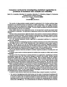
Encyclopedia of Electrical Engineering, J. G. Webster, Ed., Wiley, to appear, Feb. 1999. STATISTICAL METHODS FOR SEMICONDUCTOR MANUFACTURING DUANE S. BONING Massachusetts Institute of Technology Cambridge, MA JERRY STEFANI AND STEPHANIE W. BUTLER Texas Instruments Dallas, TX
Semiconductor manufacturing increasingly depends on the use of statistical methods in order to develop and explore new technologies, characterize and optimize existing processes, make decisions about evolutionary changes to improve yields and product quality, and monitor and maintain well-functioning processes. Each of these activities revolves around data: Statistical methods are essential in the planning of experiments to efficiently gather relevant data, the construction and evaluation of models based on data, and decision-making using these models. THE NATURE OF DATA IN SEMICONDUCTOR MANUFACTURING
An overview of the variety of data utilized in semiconductor manufacturing helps to set the context for application of the statistical methods to be discussed here. Most data in a typical semiconductor fabrication plant (or “fab”) consists of in-line and end-of-line data used for process control and material disposition. In-line data includes measurements made on wafer characteristics throughout the process (performed on test or monitor wafers, as well as product wafers), such as thicknesses of thin films after deposition, etch, or polish; critical dimensions (such as polysilicon linewidths) after lithography and etch steps; particle counts, sheet resistivities, etc. In addition to in-line wafer measurements, a large amount of data is collected on process and equipment parameters. For example, in plasma etch processes time series of the intensities of plasma emission are often gathered for use in detecting the “endpoint” (completion) of etch, and these endpoint traces (as well as numerous other parameters) are recorded. At the end-of-line, volumes of test data are taken on completed wafers. This includes both electrical test (or “etest”) data reporting parametric information about transistor and other device performance on die and scribe line structures; and sort or yield tests to identify which die on the wafer function or perform at various specifications (e.g., binning by clock speed). Such data, complemented by additional sources (e.g., fab facility environmental data, consumables or vendor data, offline equipment data) are all crucial not only for day to day monitoring and control of the fab, but also to investigate improvements, characterize the effects of uncontrolled changes (e.g., a change in wafer supply parameters), and to
redesign or optimize process steps. For correct application of statistical methods, one must recognize the idiosyncrasies of such measurements arising in semiconductor manufacturing. In particular, the usual assumptions in statistical modeling of independence and identicality of measurements often do not hold, or only hold under careful handling or aggregation of the data. Consider the measurement of channel length (polysilicon critical dimension or CD) for a particular size transistor. First, the position of the transistor within the chip may affect the channel length: Nominally identical structures may indirectly be affected by pattern dependencies or other unintentional factors, giving rise to “within die” variation. If one wishes to compare CD across multiple die on the wafer (e.g., to measure “die to die” variation), one must thus be careful to measure the same structure on each die to be compared. This same theme of “blocking” against extraneous factors to study the variation of concern is repeated at multiple length and time scales. For example, we might erroneously assume that every die on the wafer is identical, so that any random sample of, say, five die across the wafer can be averaged to give an accurate value for CD. Because of systematic wafer level variation (e.g., due to large scale equipment nonuniformities), however, each measurement of CD is likely to also be a function of the position of the die on the wafer. The average of these five positions can still be used as an aggregate indicator for the process, but care must be taken that the same five positions are always measured, and this average value cannot be taken as indicative of any one measurement. Continuing with this example, one might also take five die averages of CD for every wafer in a 25 wafer lot. Again, one must be careful to recognize that systematic wafer-to-wafer variation sources may exist. For example, in batch polysilicon deposition processes, gas flow and temperature patterns within the furnace tube will give rise to systematic wafer position dependencies; thus the 25 different five-die averages are not independent. Indeed, if one constructs a control chart under the assumption of independence, the estimate of five-die average variance will be erroneously inflated (it will also include the systematic within-lot variation), and the chart will have control limits set too far apart to detect important control excursions. If one is careful to consistently measure die-averages on the same wafers (e.g., the 6th, 12th, and 18th wafers) in each lot and aggregate these as a “lot average”, one can then construct a historical distribution of this aggregate “observation” (where an observation thus consists of several measurements) and correctly design a control chart. Great care must be taken to account for or guard against these and other systematic sources of variation which may give rise to lot-to-lot variation; these include tool dependencies, consumables or tooling (e.g., the specific reticle used in photolithography), as well as other unidentified time-dependencies. 1
Table 1: Summary of Statistical Methods Typically Used in Semiconductor Manufacturing Topic 1
Statistical Method Statistical distributions
2
Hypothesis testing
3 4
Experimental design and analysis of variance Response surface modeling
5
Categorical modeling
6
Statistical process control
Purpose Basic material for statistical tests. Used to characterize a population based upon a sample. Decide whether data under investigation indicates that elements of concern are the “same” or “different.” Determine significance of factors and models; decompose observed variation into constituent elements. Understand relationships, determine process margin, and optimize process. Use when result or response is discrete (such as “very rough,” “rough,” or “smooth”). Understand relationships, determine process margin, and optimize process. Determine if system is operating as expected.
Formal statistical assessment is an essential complement to engineering knowledge of known and suspected causal effects and systematic sources of variation. Engineering knowledge is crucial to specify data collection plans that ensure that statistical conclusions are defensible. If data is collected but care has not been not taken to make “fair” comparisons, then the results will not be trusted no matter what statistical method is employed or amount of data collected. At the same time, correct application of statistical methods are also crucial to correct interpretation of the results. Consider a simple scenario: The deposition area in a production fab has been running a standard process recipe for several months, and has monitored defect counts on each wafer. An average of 12 defects per 8 in. wafer has been observed over that time. The deposition engineer believes that a change in the gasket (from a different supplier) on the deposition vacuum chamber can reduce the number of defects. The engineer makes the change and runs two lots of 25 wafers each with the change (observing an average of 10 defects per wafer), followed by two additional lots with the original gasket type (observing an average of 11 defects per wafer). Should the change be made permanently? A “difference” in output has been observed, but a key question remains: Is the change “statistically significant”? That is to say, considering the data collected and the system’s characteristics, has a change really occurred or might the same results be explained by chance? Overview of Statistical Methods
Different statistical methods are used in semiconductor manufacturing to understand and answer questions such as that posed above and others, depending on the particular problem. Table 1 summarizes the most common methods and for what purpose they are used, and it serves as a brief outline of this article. The key engineering tasks involved in semiconductor manufacturing drawing on these methods are summarized in Table 2. In all cases, the issues of sampling plans and significance of the findings must be considered,
and all sections will periodically address these issues. To highlight these concepts, note that in Table 1 the words “different,” “same,” “good,” and “improve” are mentioned. These words tie together two critical issues: significance and engineering importance. When applying statistics to the data, one first determines if a statistically significant difference exists, otherwise the data (or experimental effects) are assumed to be the same. Thus, what is really tested is whether there is a difference that is big enough to find statistically. Engineering needs and principles determine whether that difference is “good,” the difference actually matters, or the cost of switching to a different process will be offset by the estimated improvements. The size of the difference that can be statistically seen is determined by the sampling plans and the statistical method used. Consequently, engineering needs must enter into the design of the experiments (sampling plan) so that the statistical test will be able to see a difference of the appropriate size. Statistical methods provide the means to determine sampling and significance to meet the needs of the engineer and manager. In the first section, we focus on the basic underlying issues of statistical distributions, paying particular attention to those distributions typically used to model aspects of semiconductor manufacturing, including the indispensable Gaussian distribution as well as binomial and Poisson distributions (which are key to modeling of defect and yield related effects). An example use of basic distributions is to estimate the interval of oxide thickness in which the engineer is confident that 99% of wafers will reside; based on this interval, the engineer could then decide if the process is meeting specifications and define limits or tolerances for chip design and performance modeling. In the second section, we review the fundamental tool of statistical inference, the hypothesis test as summarized in Table 1. The hypothesis test is crucial in detecting 2
Table 2: Engineering Tasks in Semiconductor Manufacturing and Statistical Methods Employed Engineering Task Process and equipment control (e.g., CDs, thickness, deposition/removal rates, endpoint time, etest and sort data, yield) Equipment matching Yield/performance modeling and prediction Debug Feasibility of process improvement
Validation of process improvement
Statistical Method Control chart for x (for wafer or lot mean) and s (for within-wafer uniformity) based on the distribution of each parameter. Control limits and control rules are based on the distribution and time patterns in the parameter. ANOVA on x and/or s over sets of equipment, fabs, or vendors. Regression of end-of-line measurement as response against in-line measurements as factors. ANOVA, categorical modeling, correlation to find most influential factors to explain the difference between good versus bad material. One-sample comparisons on limited data; single lot factorial experiment design; response surface models over a wider range of settings looking for opportunities for optimization, or to establish process window over a narrower range of settings. Two-sample comparison run over time to ensure a change is robust and works over multiple tools, and no subtle defects are incurred by change.
differences in a process. Examples include: determining if the critical dimensions produced by two machines are different; deciding if adding a clean step will decrease the variance of the critical dimension etch bias; determining if no appreciable increase in particles will occur if the interval between machine cleans is extended by 10,000 wafers; or deciding if increasing the target doping level will improve a device’s threshold voltage. In the third section, we expand upon hypothesis testing to consider the fundamentals of experimental design and analysis of variance, including the issue of sampling required to achieve the desired degree of confidence in the existence of an effect or difference, as well as accounting for the risk in not detecting a difference. Extensions beyond single factor experiments to the design of experiments which screen for effects due to several factors or their interactions are then discussed, and we describe the assessment of such experiments using formal analysis of variance methods. Examples of experimental design to enable decision-making abound in semiconductor manufacturing. For example, one might need to decide if adding an extra film or switching deposition methods will improve reliability, or decide which of three gas distribution plates (each with different hole patterns) provides the most uniform etch process. In the fourth section, we examine the construction of response surface or regression models of responses as a function of one or more continuous factors. Of particular importance are methods to assess the goodness of fit and error in the model, which are essential to appropriate use of regression models in optimization or decision-making. Examples here include determining the optimal values for temperature and pressure to produce wafers with no more than 2% nonuniformity in gate oxide thickness, or
determining if typical variations in plasma power will cause out-of-specification materials to be produced. Finally, we note that statistical process control (SPC) for monitoring the “normal” or expected behavior of a process is a critical statistical method (1,2). The fundaments of statistical distributions and hypothesis testing discussed here bear directly on SPC; further details on statistical process monitoring and process optimization can be found in SEMICONDUCTOR FACTORY CONTROL AND OPTIMIZATION. STATISTICAL DISTRIBUTIONS
Semiconductor technology development and manufacturing are often concerned with both continuous parameters (e.g., thin-film thicknesses, electrical performance parameters of transistors) and discrete parameters (e.g., defect counts and yield). In this section, we begin with a brief review of the fundamental probability distributions typically encountered in semiconductor manufacturing, as well as sampling distributions which arise when one calculates statistics based on multiple measurements (3). An understanding of these distributions is crucial to understanding hypothesis testing, analysis of variance, and other inferencing and statistical analysis methods discussed in later sections. Descriptive Statistics
“Descriptive” statistics are often used to concisely present collections of data. Such descriptive statistics are based entirely (and only) on the available empirical data, and they do not assume any underlying probability model. Such descriptions include histograms (plots of relative frequency φ i versus measured values or value ranges x i in some 3
parameter), as well as calculation of the mean: 1 x = --n
n
∑ xi
(1)
i=1
2
(where n is the number of values observed), calculation of the median (value in the “middle” of the data with an equal number of observations below and above), and calculation of data percentiles. Descriptive statistics also include the sample variance and sample standard deviation: 1 2 s x = Sample Var { x } = -----------n–1
distribution (in large part due to the central limit theorem) is the Gaussian or normal distribution. We can write that a random variable x is “distributed as” a normal distribution
n
∑ ( xi – x )
2
(2)
– 1 x – µ 2 ------ -----------σ
2 1 f ( x ) = --------------e σ 2π
s x = Sample std. dev. { x } =
x–µ normalization z = ------------ , so that z ∼ N ( 1, 0 ) : σ 1 ---
1 –2 z f ( z ) = ----------e 2π
(3)
A drawback to such descriptive statistics is that they involve the study of observed data only and enable us to draw conclusions which relate only to that specific data. Powerful statistical methods, on the other hand, have come to be based instead on probability theory; this allows us to relate observations to some underlying probability model and thus make inferences about the population (the theoretical set of all possible observations) as well as the sample (those observations we have in hand). It is the use of these models that give computed statistics (such as the mean) explanatory power. Probability Model
Perhaps the simplest probability model of relevance in semiconductor manufacturing is the Bernoulli distribution. A Bernoulli trial is an experiment with two discrete outcomes: success or failure. We can model the a priori probability (based on historical data or theoretical knowledge) of a success simply as p. For example, we may have aggregate historical data that tells us that line yield is 95% (i.e., that 95% of product wafers inserted in the fab successfully emerge at the end of the line intact). We make the leap from this descriptive information to an assumption of an underlying probability model: we suggest that the probability of any one wafer making it through the line is equal to 0.95. Based on that probability model, we can predict an outcome for a new wafer which has not yet been processed and was not part of the original set of observations. Of course, the use of such probability models involves assumptions -- for example that the fab and all factors affecting line yield are essentially the same for the new wafer as for those used in constructing the probability model. Indeed, we often find that each wafer is not independent of other wafers, and such assumptions must be examined carefully. Normal (Gaussian) Distribution. In addition to discrete probability distributions, continuous distributions also play a crucial role in semiconductor manufacturing. Quite often, one is interested in the probability density function (or pdf) for some parametric value. The most important continuous
(4)
which is also often discussed in unit normal form through the
i=1 2 sx
2
with mean µ and variance σ as x ∼ N ( µ, σ ) . The probability density function for x is given by
2
(5)
Given a continuous probability density function, one can talk about the probability of finding a value in some range. Consider the oxide thickness at the center of a wafer after rapid thermal oxidation in a single wafer system. If this oxide thickness is normally distributed with µ = 100 Å and 2
σ = 10 Å2 (or a standard deviation of 3.16 Å), then the
probability of any one such measurement x falling between 105 Å and 120 Å can be determined as 120
Pr ( 105 ≤ x ≤ 120 ) =
∫ 105
1 --------------e σ 2π
1 x–µ 2 – --- ------------ 2 σ
dx
105 – µ x – µ 120 – µ = Pr ------------------ ≤ ------------ ≤ ------------------ σ σ σ zu
= Pr ( z l ≤ z ≤ z u ) =
1 ---
2
1 –2 z dz ∫ ----------e 2π
(6)
zl
1 2 zl 1 2 zu ----1 –2 z 1 –2 z dz – ∫ ----------e dz = ∫ ----------e –∞ 2π –∞ 2π
= Φ ( zu ) – Φ ( zl ) = Φ ( 6.325 ) – Φ ( 1.581 ) = 0.0569
where Φ ( z ) is the cumulative density function for the unit normal, which is available via tables or statistical analysis packages. We now briefly summarize other common discrete probability mass functions (pmf’s) and continuous probability density functions (pdf’s) that arise in semiconductor manufacturing, and then we turn to sampling distributions that are also important. Binomial Distribution. Very often we are interested in the number of successes in repeated Bernoulli trials (that is, repeated “succeed” or “fail” trials). If x is the number of successes in n trials, then x is distributed as a binomial distribution x ∼ B ( n, p ) , where p is the probability of each individual “success”. The pmf is given by
4
n–x n x f ( x, p, n ) = p ( 1 – p ) x
(7)
where “n choose x” is n! n = ---------------------- x x! ( n – x )!
(8)
For example, if one is starting a 25-wafer lot in the fab above, one may wish to know what is the probability that some number x (x being between 0 and 25) of those wafers will survive. For the line yield model of p = 95%, these probabilities are shown in Fig. 1. When n is very large (much larger than 25), the binomial distribution is well approximated by a Gaussian distribution.
0.4 0.35 0.3
are Poisson-distributed with a mean defect count of 3 particles per 200 mm wafer, one can ask questions about the probability of observing x [e.g., Eq. (9)] defects on a sample –3 9
wafer. In this case, f ( 9, 3 ) = ( e 3 ) ⁄ 9! = 0.0027 , or less than 0.3% of the time would we expect to observe exactly 9 defects. Similarly, the probability that 9 or more defects are 8
observed is 1 –
∑
f ( x, 3 ) = 0.0038 .
x=0
In the case of defect modeling, several other distributions have historically been used, including the exponential, hypergeometric, modified Poisson, and negative binomial. Substantial additional work has been reported in yield modeling to account for clustering, and to understand the relationship between defect models and yield (e.g., see Ref. 4).
0.25
Population Versus Sample Statistics 0.2 0.15 0.1 0.05 0 0
5
10 Wafers
15
20
25
surviving
We now have the beginnings of a statistical inference theory. Before proceeding with formal hypothesis testing in the next section, we first note that the earlier descriptive statistics of mean and variance take on new interpretations in the probabilistic framework. The mean is the expectation (or “first moment”) over the distribution: ∞
µx = E{ x } =
Figure 1. Probabilities for number of wafers surviving from a lot of 25 wafers, assuming a line yield of 90%, calculated using the binomial distribution. A key assumption in using the Bernoulli distribution is that each wafer is independent of the other wafers in the lot. One often finds that many lots complete processing with all wafers intact, and other lots suffer multiple damaged wafers. While an aggregate line yield of 95% may result, independence does not hold and alternative approaches such as formation of empirical distributions should be used.
–∞
–λ x
e λ f ( x, λ ) = -------------x!
(9)
for integer λ = 0, 1, 2, … and λ ≅ np . For example, one can examine the number of chips that fail on the first day of operation: The probability p of failure for any one chip is (hopefully) exceedingly small, but one tests a very large number n of chips, so that the observation of the mean number of failed chips λ = np is Poisson distributed. An even more common application of the Poisson model is in defect modeling. For example, if defects
(10)
n
=
∑ xi ⋅ pr ( xi ) i=1
for continuous pdf’s and discrete pmf’s, respectively. Similarly, the variance is the expectation of the squared deviation from the mean (or the “second central moment”) over the distribution: ∞ 2
σ x = Var { x } =
∫ ( x – E{ x })
2
f ( x ) dx
–∞
(11)
n
Poisson Distribution. A third discrete distribution is highly
relevant to semiconductor manufacturing. An approximation to the binomial distribution that applies when n is large and p is small is the Poisson distribution:
∫ xf ( x ) dx
=
∑ ( xi – E { xi } )
2
⋅ pr ( xi )
i=1
Further definitions from probability theory are also highly useful, including the covariance: 2
σ xy = Cov { x, y } = E { ( x – E { x } ) ( y – E { y } ) }
(12)
= E { xy } – E { x }E { y }
where x and y are each random variables with their own probability distributions, as well as the related correlation coefficient: 2
σ xy Cov { x, y } ρ xy = Corr { x, y } = ------------------------------------------ = ----------σxσy Var { x }Var { y }
(13)
The above definitions for the mean, variance, covariance, and correlation all relate to the underlying or 5
assumed population. When one only has a sample (that is, a finite number of values drawn from some population), one calculates the corresponding sample statistics. These are no longer “descriptive” of only the sample we have; rather, these statistics are now estimates of parameters in a probability model. Corresponding to the population parameters above, the sample mean x is given by Eq. (1), the sample variance
2 sx
lying within particular ranges, we must be sure to use the distribution for T rather than that for the underlying distribution T. Thus, in this case the probability of finding a value T between 105 Å and 120 Å is Pr ( 105 ≤ T ≤ 120 ) 105 – µ T–µ 120 – µ = Pr ------------------- ≤ ------------------- ≤ ------------------- σ ⁄ ( n ) σ ⁄ ( n ) σ ⁄ ( n )
by Eq. (2), the sample std. dev. s x by Eq.
105 – 100 T–µ 120 – 100 = Pr ------------------------------- ≤ ------------------- ≤ ------------------------ ( 10 ) ⁄ ( 5 ) σ ⁄ ( n ) 2 = Pr ( z l ≤ z ≤ z u )
(3), the sample covariance is given by 1 2 s xy = -----------n–1
n
∑ ( xi – x ) ( yi – y )
(14)
= Φ ( 14.142 ) – Φ ( 3.536 ) = 0.0002
i=1
and the sample correlation coefficient is given by r xy
s xy = --------sxsy
(15)
Sampling Distributions
Sampling is the act of making inferences about populations based on some number of observations. Random sampling is especially important and desirable, where each observation is independent and identically distributed. A statistic is a function of sample data which contains no further unknowns (e.g., the sample mean can be calculated from the observations and has no further unknowns). It is important to note that a sample statistic is itself a random variable and has a “sampling distribution” which is usually different than the underlying population distribution. In order to reason about the “likelihood” of observing a particular statistic (e.g., the mean of five measurements), one must be able to construct the underlying sampling distribution. Sampling distributions are also intimately bound up with estimation of population distribution parameters. For example, suppose we know that the thickness of gate oxide (at the center of the wafer) is normally distributed: 2
T i ∼ N ( µ, σ ) = N ( 100, 10 ) . We sample five random wafers
and
compute
the
mean
oxide
(17)
thickness
1 T = --- ( T 1 + T 2 + … + T 5 ) . We now have two key questions: 5
which is relatively unlikely. Compare this to the result from Eq. (6) for the probability 0.0569 of observing a single value (rather than a five sample average) in the range 105 Å to 120 Å. Note that the same analysis would apply if T i was itself formed as an average of underlying oxide thickness measurements (e.g., from a nine point pattern across the wafer), if that average T i ∼ N ( 100, 10 ) and each of the five wafers used in calculating the sample average T are independent and also distributed as N ( 100, 10 ) . Chi-Square Distribution and Variance Estimates. Several other vitally important distributions arise in sampling, and are essential to making statistical inferences in experimental design or regression. The first of these is the chi-square distribution. If x i ∼ N ( 0, 1 ) for i = 1, 2, …, n and 2
2
2
y = x 1 + x 2 + … + x n , then y is distributed as chi-square with 2
n degrees of freedom, written as y ∼ χ n . While formulas for 2
the probability density function for χ exist, they are almost never used directly and are again instead tabulated or 2
available via statistical packages. The typical use of the χ is for finding the distribution of the variance when the mean is known.
(1) What is the distribution of T ? (2) What is the probability 2
Suppose we know that x i ∼ N ( µ, σ ) . As discussed
that a ≤ T ≤ b ?
previously, we know that the mean over our n observations is In this case, given the expression for T above, we can use the fact that the variance of a scaled random variable ax
2
2
2
is simply a Var { x } , and the variance of a sum of independent random variables is the sum of the variances 2
T ∼ N ( µ, σ ⁄ n )
(16) where µ T = µ T = µ by the definition of the mean. Thus,
2
distributed as x ∼ N ( µ, σ ⁄ n ) . How is the sample variance s over our n observations distributed? We note that each ( x i – x ) ∼ N ( 0, σ )
is normally distributed; thus if we
normalize our sample variance s square distribution:
2
by σ
2
we have a chi-
when we want to reason about the likelihood of observing values of T (that is, averages of five sample measurements) 6
y ⁄u y2 ⁄ v
2 2 s = ∑ ( xi – x ) ⁄ ( n – 1 )
2 1 - ∼ F u, v similarly y 2 ∼ χ v , then the random variable Y = -----------
i
2
( n – 1 )s 2 ---------------------- ∼ χ n – 1 2 σ 2
(18)
2
σ 2 s ∼ ---------------- ⋅ χ (n – 1) n–1
where one degree of freedom is used in calculation of x . Thus, the sample variance for n observations drawn from 2
N ( µ, σ ) is distributed as chi-square as shown in Eq. (18).
For our oxide thickness example where T i ∼ N ( 100, 10 ) 2
2
and we form sample averages T as above, then s T ∼ 10χ 4 ⁄ 4 and 95% of the time the observed sample variable will be less than 1.78 Å2. A control chart could thus be constructed to detect when unusually large five-wafer sample variances occur. Student t Distribution. The Student t distribution is another important sampling distribution. The typical use is when we want to find the distribution of the sample mean when the true standard deviation σ is not known. Consider 2
x i ∼ N ( µ, σ ) x–µ ----------------- σ ⁄ ( n ) N ( 0, 1 ) x–µ ------------------ = ------------------------- ∼ ----------------------------- ∼ t n – 1 s⁄σ 1 2 s ⁄ ( n) ------------ χ n – 1 n–1
(19)
In the above, we have used the definition of the Student t distribution: if z is a random variable, z ∼ N ( 0, 1 ) , then z ⁄ ( y ⁄ k ) is distributed as a Student t with k degrees of
freedom, or z ⁄ ( y ⁄ k ) ∼ t k , if y . is a random variable 2
distributed as χ k . As discussed previously, the normalized 2
(that is, distributed as F with u and v degrees of freedom). The typical use of the F distribution is to compare the spread of two distributions. For example, suppose that we have two samples and where w 1, w 2, …, w m , x 1, x 2, …, x n 2
2
x i ∼ N ( µ x, σ x ) and w i ∼ N ( µ w, σ w ) . Then 2
2
sx ⁄ σx --------------- ∼ F n – 1, m – 1 2 2 sw ⁄ σw
(20)
Point and Interval Estimation
The above population and sampling distributions form the basis for the statistical inferences we wish to draw in many semiconductor manufacturing examples. One important use of the sampling distributions is to estimate population parameters based on some number of observations. A point estimate gives a single “best” estimated value for a population parameter. For example, the sample mean x is an estimate for the population mean µ . Good point estimates are representative or unbiased (that is, the expected value of the estimate should be the true value), as well as minimum variance (that is, we desire the estimator with the smallest variance in that estimate). Often we restrict ourselves to linear estimators; for example, the best linear unbiased estimator (BLUE) for various parameters is typically used. Many times we would like to determine a confidence interval for estimates of population parameters; that is, we want to know how likely it is that x is within some particular range of µ . Asked another way, to a desired probability, where will µ actually lie given an estimate x ? Such interval estimation is considered next; these intervals are used in later sections to discuss hypothesis testing.
2
sample variance s ⁄ σ is chi-square-distributed, so that our definition does indeed apply. We thus find that the normalized sample mean is distributed as a Student t with n1 degrees of freedom when we do not know the true standard deviation and must estimate it based on the sample as well. We note that as k → ∞ , the Student t approaches a unit normal distribution t k → N ( 0, 1 ) . F Distribution and Ratios of Variances. The last sampling
distribution we wish to discuss here is the F distribution. We shall see that the F distribution is crucial in analysis of variance (ANOVA) and experimental design in determining the significance of effects, because the F distribution is concerned with the probability density function for the ratio 2
of variances. If y 1 ∼ χ u (that is, y 1 is a random variable distributed as chi-square with u degrees of freedom) and
First, let us consider the confidence interval for estimation of the mean, when we know the true variance of the process. Given that we make n independent and identically distributed samples from the population, we can calculate the sample mean as in Eq. (1). As discussed earlier, we know that the sample mean is normally distributed as shown in Eq. (16). We can thus determine the probability that an observed x is larger than µ by a given amount: x–µ z = ------------------σ ⁄ ( n) Pr ( z > z α ) = α = 1 – Φ ( z α )
(21)
where z α is the alpha percentage point for the normalized variable z (that is, z α measures how many standard deviations greater than µ we must be in order for the 7
integrated probability density to the right of this value to equal α ). As shown in Fig. 2, we are usually interested in asking the question the other way around: to a given probability [ 100 ( 1 – α ) , e.g., 95%], in what range will the true mean lie given an observed x ? σ σ x – z α ⁄ 2 ⋅ ------- ≤ µ ≤ x + z α ⁄ 2 ⋅ ------- n n σ µ = x ± z α ⁄ 2 ⋅ ------n
(22)
.
2
f ( x ) ∼ N ( µ, σ ⁄ n )
α⁄2
µ
x
α⁄2
x
2
2
( n – 1 )s ( n – 1 )s 2 ----------------------- ≤ σ ≤ -----------------------------2 2 χ α ⁄ 2, n – 1 χ 1 – α ⁄ 2, n – 1
(25)
For example, consider a new etch process which we want to characterize. We calculate the average etch rate (based on 21-point spatial pre- and post-thickness measurements across the wafer) for each of four wafers we process. The wafer averages are 502, 511, 515, and 504 Å/ min. The sample mean is x = 511 Å/min, and the sample standard deviation is s = 6.1 Å/min. The 95% confidence intervals for the true mean and std. dev. are µ = 511 ± 12.6 Å/min, and 3.4 ≤ σ ≤ 22.6 Å/min. Increasing the number of observations (wafers) can improve our estimates and intervals for the mean and variance, as discussed in the next section. Many other cases (e.g., one-sided confidence intervals) can also be determined based on manipulation of the appropriate sampling distributions, or through consultation with more extensive texts (5). HYPOTHESIS TESTING
Figure 2. Probability density function for the sample mean. The sample mean is unbiased (the expected value of the sample mean is the true mean µ ). The shaded portion in the tail captures the probability that the sample mean is greater than a distance x – µ from the true mean. For our oxide thickness example, we can now answer an important question. If we calculate a five-wafer average, how far away from the average 100 Å must the value be for us to decide that the process has changed away from the mean (given a process variance of 10 Å2)? In this case, we must define the “confidence” 1 – α in saying that the process has changed; this is equivalent to the probability of observing the deviation by chance. With 95% confidence, we can declare that the process is different than the mean of 100 Å if we observe T < 97.228 Å or T > 102.772 Å: T–µ T–µ α ⁄ 2 = Pr z α ≤ ------------------- = Pr – 1.95996 ≤ ------------------- -σ ⁄ ( n ) (23) 2 σ ⁄ ( n ) T – µ = 1.95996σ ⁄ ( n ) = 2.7718
A similar result occurs when the true variance is not known. The 100 ( 1 – α ) confidence interval in this case is determined using the appropriate Student t sampling distribution for the sample mean: s s x – t α ⁄ 2, n – 1 ⋅ ------- ≤ µ ≤ x + t α ⁄ 2, n – 1 ⋅ ------- n n s µ = x ± t α ⁄ 2, n – 1 ⋅ ------n
(24)
In some cases, we may also desire a confidence interval on the estimate of variance:
Given an underlying probability distribution, it now becomes possible to answer some simple, but very important, questions about any particular observation. In this section, we formalize the decision-making earlier applied to our oxide thickness example. Suppose as before that we know that oxide thickness is normally distributed, with a mean of 100 Å and standard deviation of 3.162 Å. We may know this based on a very large number of previous historical measurements, so that we can well approximate the true population of oxide thicknesses out of a particular furnace with these two distribution parameters. We suspect something just changed in the equipment, and we want to determine if there has been an impact on oxide thickness. We take a new observation (i.e., run a new wafer and form our oxide thickness value as usual, perhaps as the average of nine measurements at fixed positions across the wafer). The key question is: What is the probability that we would get this observation if the process has not changed, versus the probability of getting this observation if the process has indeed changed? We are conducting a hypothesis test. Based on the observation, we want to test the hypothesis (label this H1) that the underlying distribution mean has increased from µ 0 by some amount δ to µ 1 . The “null hypothesis” H0 is that nothing has changed and the true mean is still µ 0 . We are looking for evidence to convince us that H1 is true. We can plot the probability density function for each of the two hypotheses under the assumption that the variance has not changed, as shown in Fig. 3. Suppose now that we 8
observe the value x i . Intuitively, if the value of x i is “closer” to µ 0 than to µ 1 , we will more than likely believe that the value comes from the H0 distribution than the H1 distribution. Under a maximum likelihood approach, we can compare the probability density functions: H0 f 0 ( xi ) > < f 1 ( xi ) H1
(26)
that is, if f 1 is greater than f 0 for our observation, we reject the null hypothesis H0 (that is, we “accept” the alternative hypothesis H1). If we have prior belief (or other knowledge) affecting the a priori probabilities of H0 and H1, these can also be used to scale the distributions f 0 and f 1 to determine a posterior probabilities for H0 and H1. Similarly, we can define the “acceptance region” as the set of values of x i for which we accept each respective hypothesis. In Fig. 3,
averages, then we must observe T < 97.2 Å or T > 102.8 Å as in Eq. (23) to convince us (to 95% confidence) that our process has changed. Alpha and Beta Risk (Type I and Type II Errors)
The hypothesis test gives a clear, unambiguous procedure for making a decision based on the distributions and assumptions outlined above. Unfortunately, there may be a substantial probability of making the wrong decision. In the maximum likelihood example of Fig. 3, for the single observation x i as drawn we accept the alternative hypothesis H1. However, examining the distribution corresponding to H0, we see that a nonzero probability exists of x i belonging to H1.Two types of errors are of concern: α = Pr (Type I error) ∞
*
we have the rule: accept H1 if x i > x , and accept H0 if
∫ f 0 ( x ) dx
= Pr ( reject H 0 H 0 is true ) =
x*
*
xi < x .
(27)
β = Pr (Type II error) x*
= Pr ( accept H 0 H 1 is true ) =
∫
f 1 ( x ) dx
–∞
2
H 0 : f 0 ( x ) ∼ N ( µ 0, σ )
x µ0
*
δ
xi
x
µ1
Figure 3. Distributions of x under the null hypothesis H0, and under the hypothesis H1 that a positive shift has occurred such that µ 1 = µ 0 + δ . The maximum likelihood approach provides a powerful but somewhat complicated means for testing hypotheses. In typical situations, a simpler approach suffices. We select a confidence 1 – α with which we must detect a “difference,” *
and we pick a x decision point based on that confidence. For two-sided detection with a unit normal distribution, for example, we select z > z α ⁄ 2 and z < – z α ⁄ 2 as the regions for declaring that unusual behavior (i.e., a shift) has occurred. Consider our historical data on oxide thickness where T i ∼ N ( 100, 10 ) . To be 95% confident that a new observation
indicates a change in mean, we must observe T i < 93.8 Å or T i > 106.2 Å. On the other hand, if we form five-wafer
We note that the Type I error (or probability α of a “false alarm”) is based entirely on our decision rule and does not depend on the size of the shift we are seeking to detect. The Type II error (or probability β of “missing” a real shift), on the other hand, depends strongly on the size of the shift. This Type II error can be evaluated for the distributions and decision rules above; for the normal distribution of Fig. 3, we find δ δ β = Φ z α ⁄ 2 – --- – Φ – z α ⁄ 2 – --- σ σ
(28)
where δ is the shift we wish to detect. The “power” of a statistical test is defined as Power ≡ 1 – β = Pr ( reject H 0 H 0 is false )
(29)
that is, the power of the test is the probability of correctly rejecting H0. Thus the power depends on the shift δ we wish to detect as well as the level of “false alarms” ( α or Type I error) we are willing to endure. Power curves are often plotted of β versus the normalized shift to detect d = δ ⁄ σ , for a given fixed α (e.g., α = 0.05 ), and as a function of sampling size. Hypothesis Testing and Sampling Plans. In the previous discussion, we described a hypothesis test for detection of a shift in mean of a normal distribution, based on a single observation. In realistic situations, we can often make multiple observations and improve our ability to make a correct decision. If we take n observations, then the sample
9
mean is normally distributed, but with a reduced variance 2
σ ⁄ n as illustrated by our five-wafer average of oxide thickness. It now becomes possible to pick an α risk associated with a decision on the sampling distribution that is acceptable, and then determine a sample size n in order to achieve the desired level of β risk. In the first step, we still select z α ⁄ 2 based on the risk of false alarm α , but now this
determines the actual unnormalized decision point using *
x = µ + z α ⁄ 2 ⋅ σ ⁄ ( n ) . We finally pick n (which determines *
as just defined) based on the Type II error, which also depends on the size of the normalized shift d = δ ⁄ σ to be detected and the sample size n. Graphs and tables are indispensable in selecting the sample size for a given d and α ; for example, Fig. 4 shows the Type II error associated with sampling from a unit normal distribution, for a fixed Type I error of 0.05, and as a function of sampling size n and shift to be detected d. x
Control Chart Application. The concepts of hypothesis testing, together with issues of Type I and Type II error as well as sample size determination, have one of their most common applications in the design and use of control charts.
For example, the x control chart can be used to detect when a “significant” change from “normal” operation occurs. The assumption here is that when the underlying process is operating under control, the fundamental process population 2
is distributed normally as x i ∼ N ( µ, σ ) . We periodically draw a sample of n observations and calculate the average of those observations ( x ). In the control chart, we essentially perform a continuous hypothesis test, where we set the upper and lower control limits (UCLs and LCLs) such that x falls outside these control charts with probability α when the process is truly under control (e.g., we usually select 3σ to give a 0.27% chance of false alarm). We would then choose the sample size n so as to have a particular power (that is, a probability of actually detecting a shift of a given size) as previously described. The control limits (CLs) would then be set at σ CL = µ ± z α ⁄ 2 ⋅ ------- n
1 0.9 0.8
(30)
n=2 0.7
n=3
0.6
n=5
0.5
n = 10 n = 20
0.4
n = 30
0.3
n = 40 0.2 0.1 0 0
0.5
1
1.5
2
Delta (in units of standard deviation)
Figure 4. Probability of Type II error ( β ) for a unit normal process with Type I error fixed at α = 0.05 , as a function of sample size n and shift delta (equal to the normalized shift δ ⁄ σ ) to be detected. Consider once more our wafer average oxide thickness T i . Suppose that we want to detect a 1.58 Å (or 0.5 σ ) shift
from the 100 Å mean. We are willing to accept a false alarm 5% of the time ( α = 0.05 ) but can accept missing the shift 20% of the time ( β = 0.20 ). From Fig. 4, we need to take n = 30 . Our decision rule is to declare that a shift has occurred if our 30 sample average T < 98.9 Å or T > 101.1 Å. If it is even more important to detect the 0.5 σ shift in mean (e.g., with probability β = 0.10 of missing the shift), then from Fig. 4 we now need n = 40 samples, and our decision rule is to declare a shift if the 40 sample average T < 99.0 Å or T > 101.0 Å.
Note that care must be taken to check key assumptions in setting sample sizes and control limits. In particular, one should verify that each of the n observations to be utilized in forming the sample average (or the sample standard deviation in an s chart) are independent and identically distributed. If, for example, we aggregate or take the average of n successive wafers, we must be sure that there are no systematic within-lot sources of variation. If such additional variation sources do exist, then the estimate of variance formed during process characterization (e.g., in our etch example) will be inflated by accidental inclusion of this systematic contribution, and any control limits one sets will be wider than appropriate to detect real changes in the underlying random distribution. If systematic variation does indeed exist, then a new statistic should be formed that blocks against that variation (e.g., by specifying which wafers should be measured out of each lot), and the control chart based on the distribution of that aggregate statistic. EXPERIMENTAL DESIGN AND ANOVA
In this section, we consider application and further development of the basic statistical methods already discussed to the problem of designing experiments to investigate particular effects, and to aid in the construction of models for use in process understanding and optimization. First, we should recognize that the hypothesis testing methods are precisely those needed to determine if a new treatment induces a significant effect in comparison to a process with a known distribution. These are known as onesample tests. In this section, we next consider two-sample 10
tests to compare two treatments in an effort to detect a treatment effect. We will then extend to the analysis of experiments in which many treatments are to be compared (k-sample tests), and we present the classic tool for studying the results --- ANOVA (6). Comparison of Treatments: Two-Sample Tests
Consider an example where a new process B is to be compared against the process of record (POR), process A. In the simplest case, we have enough historical information on process A that we assume values for the yield mean µ A and standard deviation σ . If we gather a sample of 10 wafers for the new process, we can perform a simple one-sample hypothesis test µ B > µ A using the 10 wafer sampling distribution and methods already discussed, assuming that both process A and B share the same variance. Consider now the situation where we want to compare two new processes. We will fabricate 10 wafers with process A and another 10 wafers with process B, and then we will measure the yield for each wafer after processing. In order to block against possible time trends, we alternate between process A and process B on a wafer by wafer basis. We are seeking to test the hypothesis that process B is better than process A, that is H1: µ B > µ A , as opposed to the null hypothesis H0: µ B = µ A . Several approaches can be used (5). In the first approach, we assume that in each process A and B we are random sampling from an underlying normal distribution, with (1) an unknown mean for each process and (2) a constant known value for the population standard deviation
of
σ.
Then
2
n A = 10 ,
n B = 10 ,
2
Var { y A } = σ ⁄ n A , and Var { y B } = σ ⁄ n B . We can then
construct the sampling distribution for the difference in means as 2
2
2 1 σ σ 1 Var { y B – y A } = ------ + ------ = σ ------ + ------ n A n B nA nB
(31)
1 1 s B – A = σ ------ + -----nA nB
(32)
Even if the original process is moderately non-normal, the distribution of the difference in sample means will be approximately normal by the central limit theorem, so we can normalize as ( yB – yA) – (µB – µA) z 0 = ---------------------------------------------------1 1 σ ------ + -----nA nB
(33)
allowing us to examine the probability of observing the mean difference y B – y A based on the unit normal
distribution, Pr ( z > z 0 ) . The disadvantage of the above method is that it depends on knowing the population standard deviation σ . If such information is indeed available, using it will certainly improve the ability to detect a difference. In the second approach, we assume that our 10 wafer samples are again drawn by random sampling on an underlying normal population, but in this case we do not assume that we know a priori what the population variance is. In this case, we must also build an internal estimate of the variance. First, we estimate σ from the individual variances: 2 sA
1 = --------------nA – 1
nA
∑ ( yA – yA)
(34)
i
i=1
2
and similarly for s B . The pooled variance is then 2
2
( n A – 1 )s A + ( n B – 1 )s B 2 s = --------------------------------------------------------nA + nB – 2
(35)
Once we have an estimate for the population variance, we can perform our t test using this pooled estimate: ( yB – yA) – (µB – µA) t 0 = ---------------------------------------------------1 1 s ------ + -----nA nB
(36)
One must be careful in assuming that process A and B share a common variance; in many cases this is not true and more sophisticated analysis is needed (5). Comparing Several Treatment Means via ANOVA
In many cases, we are interested in comparing several treatments simultaneously. We can generalize the approach discussed above to examine if the observed differences in treatment means are indeed significant, or could have occurred by chance (through random sampling of the same underlying population). A picture helps explain what we are seeking to accomplish. As shown in Fig. 5, the population distribution for each treatment is shown; the mean can differ because the treatment is shifted, while we assume that the population variance is fixed. The sampling distribution for each treatment, on the other hand, may also be different if a different number of samples is drawn from each treatment (an “unbalanced” experiment), or because the treatment is in fact shifted. In most of the analyses that follow, we will assume balanced experiments; analysis of the unbalanced case can also be performed (7). It remains important to recognize that particular sample values from the sampling distributions are what we measure. In essence, we must compare the variance between two groups (a measure of the potential “shift” between treatments) with the variance within each group (a measure of the sampling variance). Only if the shift is “large” compared to the sampling 11
variance are we confident that a true effect is in place. An appropriate sample size must therefore be chosen using methods previously described such that the experiment is powerful enough to detect differences between the treatments that are of engineering importance. In the following, we discuss the basic methods used to analyze the results of such an experiment (8).
measurements, N = n 1 + n 2 + … + n k , or simply N = nk if all k treatments consist of the same number of samples, n . In the second step, we want an estimate of betweengroup variation. We will ultimately be testing the hypothesis µ 1 = µ 2 = … = µ k . The estimate of the between-group variance is k
∑ nt ( yt – y )
2
y
sT =
Population distributions
yB
t=1
2
SS = --------TυT
(40)
where SS T ⁄ υ T is defined as the between treatment mean square, υ T = k – 1 , and y is the overall mean.
yC
We are now in position to ask our key question: Are the treatments different? If they are indeed different, then the between-group variance will be larger than the within-group variance. If the treatments are the same, then the betweengroup variance should be the same as the within-group variance. If in fact the treatments are different, we thus find that
yA
A
B
C
2
Figure 5. Pictorial representation of multiple treatment experimental analysis. The underlying population for each treatment may be different, while the variance for each treatment population is assumed to be constant. The dark circles indicate the sample values drawn from these populations (note that the number of samples may not be the same in each treatment). First, we need an estimate of the within-group variation. Here we again assume that each group is normally 2
distributed and share a common variance σ . Then we can form the “sum of squares” deviations within the tth group SS t as nt
SS t =
∑ ( yt
j
– yt )
2
(37)
2 sT
k nt τt 2 - estimates σ + ∑ --------------( k – 1 ) t=1
2
where τ t = µ t – µ is treatment t’s effect. That is, s T is inflated by some factor related to the difference between treatments. We can perform a formal statistical test for treatment significance. Specifically, we should consider the evidence to be strong for the treatments being different if the 2
2
ratio s T ⁄ s R is significantly larger than 1. Under our assumptions, this should be evaluated using the F 2
2
distribution, since s T ⁄ s R ∼ F k – 1, N – k . We can also express the total variation (total deviation sum of squares from the grand mean SS D ) observed in the data as
j=1
k
where n t is the number of observations or samples in group
SS D =
t. The estimate of the sample variance for each group, also referred to as the “mean square,” is thus SS t SS 2 s t = -------t = -----------υt nt – 1
(38)
where υ t is the degrees of freedom in treatment t. We can generalize the pooling procedure used earlier to estimate a common shared variance across k treatments as 2
2
2
SS R SS υ1 s1 + υ2 s2 + … + υk sk 2 - = --------Rs R = ---------------------------------------------------------= -----------υ1 + υ2 + … + υk N–k υR
(39)
where SS R ⁄ υ R is defined as the within-treatment or withingroup mean square and N
(41)
nt
∑ ∑ ( yti – y
2
)
(42)
t=1 i=1 2 sD
SS D SS D = --------- = -----------υD N–1
2
where s D is recognized as the variance in the data. Analysis of variance results are usually expressed in tabular form, such as shown in Table 3. In addition to compactly summarizing the sum of squares due to various components and the degrees of freedom, the appropriate F ratio is shown. The last column of the table usually contains the probability of observing the stated F ratio under the null hypothesis. The alternative hypothesis --- that one or more
is the total number of 12
Table 3: Structure of the Analysis of Variance Table, for Single Factor (Treatment) Case Source of Variation
Sum of Squares
Degrees of Freedom
Between treatments
SS T
υT = k – 1
sT
Within treatments
SS R
υR = N – k
sR
Total about the grand mean
SS D = SS T + SS R
υ D = υT + υ R = N – 1
sD
treatments have a mean different than the others --- can be accepted with 100 ( 1 – p ) confidence. As summarized in Table 3, analysis of variance can also be pictured as a decomposition of the variance observed in the data. That is, we can express the total sum of squared deviations from the grand mean as SS D = SS T + SS R , or the between-group sum of squares added to the within-group sum of squares. We have presented the results here around the grand mean. In some cases, an alternative presentation is 2
2
2
Mean Square
F ratio
2
sT ⁄ s R
2
Pr(F)
2
p
2
2
especially alert to dependencies on the size of the estimate (e.g., proportional versus absolute errors). Finally, one should also plot the residuals against any other variables of interest, such as environmental factors that may have been recorded. If unusual behavior is noted in any of these steps, additional measures should be taken to stabilize the variance (e.g., by considering transformations of the variables or by reexamining the experiment for other factors that may need to be either blocked against or otherwise included in the experiment).
used where a “total” sum of squares SS = y 1 + y 2 + … + y N
Two-Way Analysis of Variance
is used. In this case the total sum of squares also includes
Suppose we are seeking to determine if various treatments are important in determining an output effect, but we must conduct our experiment in such a way that another variable (which may also impact the output) must also vary. For example, suppose we want to study two treatments A and B but must conduct the experiments on five different process tools (tools 1-5). In this case, we must carefully design the experiment to block against the influence of the process tool factor. We now have an assumed model: (45) y ti = µ + τ t + β i + ε ti
variation
due
to
the
average,
2
SS A = N y ,
or
SS = SS A + SS D = SS A + SS T + SS R . In Table 3, k is the
number of treatments and N is the total number of 2
2
observations. The F ratio value is s T ⁄ s R , which is compared against the F ratio for the degrees of freedom υ T and υ R . The
p
Pr( F υT, υ R >
value 2 sT
⁄
2 sR
shown
in
such
a
table
is
µ 1 = … = µ k ).
where β i are the block effects. The total sum of squares SS While often not explicitly stated, the above ANOVA assumes a mathematical model: y ti = µ t + ε ti = µ + τ t + ε ti (43) where µ t are the treatment means, and ε ti are the residuals: 2
ε ti = y ti – yˆti ∼ N ( 0, σ )
(44)
where yˆti = yˆt = µ + τ t is the estimated treatment mean. It is critical that one check the resulting ANOVA model. First, the residuals ε ti should be plotted against the time order in which the experiments were performed in an attempt to distinguish any time trends. While it is possible to randomize against such trends, we lose resolving power if the trend is large. Second, one should examine the distribution of the residuals. This is to check the assumption that the residuals are “random” [that is, independent and identically distributed (IID) and normally distributed with zero mean] and look for gross non-normality. This check should also include an examination of the residuals for each treatment group. Third, one should plot the residuals versus the estimates and be
can now be decomposed as (46)
SS = SS A + SS B + SS T + SS R
with degrees of freedom bk = 1 + ( b – 1 ) + ( k – 1 ) + ( b – 1 ) ( k – 1 )
(47) where b is the number of blocking groups, k is the b
number of treatment groups, and SS B = k ∑ ( y i – y ) . As 2
i=1
before, if the blocks or treatments do in fact include any mean shifts, then the corresponding mean sum of squares (estimates of the corresponding variances) will again be inflated beyond the population variance (assuming the number of samples at each treatment is equal): b
2
βi 2 2 s B estimates σ + k ∑ --------------- ( b – 1 ) i=1
(48)
2
2 sT
k nt τt 2 - estimates σ + ∑ --------------( k – 1 ) t=1
13
Table 4: Structure of the Analysis of Variance Table, for the Case of a Treatment with a Blocking Factor Source of Variation Average (correction factor)
Sum of Squares SS A = nk y
Between blocks
∑ ( yi – y )
Mean Square
F ratio
Pr(F)
1
2
b
SS B = k
Degrees of Freedom
2
υB = b – 1
sB
2
sB ⁄ sR
2
υT = k – 1
sT
2
sT ⁄ s R
2
2
pB
2
2
pT
i=1
Between treatments
k
SS T = b ∑ ( y t – y ) t=1
Residuals
SS R
υR = (b – 1)(k – 1)
sR
Total
SS
υ = N = bk
sD
where we assume that k samples are observed for each of the b blocks. So again, we can now test the significance of these potentially “inflated” variances against the pooled estimate 2
of the variance s R with the appropriate F test as summarized in Table 4. Note that in Table 4 we have shown the ANOVA table in the non-mean centered or “uncorrected” format, so that SS A due to the average is shown. The table can be converted to the mean corrected form as in Table 3 by removing the SS A row, and replacing the total SS with the mean corrected total SS D with υ = N – 1 degrees of freedom. Two-Way Factorial Designs
While the above is expressed with the terminology of the second factor being considered a “blocking” factor, precisely the same analysis pertains if two factors are simultaneously considered in the experiment. In this case, the blocking groups are the different levels of one factor, and the treatment groups are the levels of the other factor. The assumed analysis of variance above is with the simple additive model (that is, assuming that there are no interactions between the blocks and treatments, or between the two factors). In the blocked experiment, the intent of the blocking factor was to isolate a known (or suspected) source of “contamination” in the data, so that the precision of the experiment can be improved. We can remove two of these assumptions in our experiment if we so desire. First, we can treat both variables as equally legitimate factors whose effects we wish to identify or explore. Second, we can explicitly design the experiment and perform the analysis to investigate interactions between the two factors. In this case, the model becomes (49) y tij = µ ti + ε tij
2
2
where µ ti is the effect that depends on both factors simultaneously. The output can also be expressed as µ ti = µ + τ t + β i + ω ti
(50)
= y + ( y t – y ) + ( y i – y ) + ( y ti – y t – y i + y )
where µ is the overall grand mean, τ t and β i are the main effects, and ω ti are the interaction effects. In this case, the subscripts are t = 1, 2, …, k i = 1, 2, …, b j = 1, 2, …, m
where k is the # levels of first factor where b is the # levels of second factor where m is the # replicates at t, i factor
The resulting ANOVA table will be familiar; the one key addition is explicit consideration of the interaction sum of squares and mean square. The variance captured in this component can be compared to the within-group variance as before, and be used as a measure of significance for the interactions, as shown in Table 5. Another metric often used to assess “goodness of fit” of a model is the R2. The fundamental question answered by R2 is how much better does the model do than simply using the grand average. SS M ( SS T + SS B + SS I ) 2 R = --------- = -------------------------------------------SS D SS D
(51)
where SS D is the variance or sum of square deviations around the grand average, and SS M is the variance captured by the model consisting of experimental factors ( SS T and SS B ) and interactions ( SS I ). An R2 value near zero indicates
that most of the variance is explained by residuals ( SS R = SS D – SS M ) rather than by the model terms ( SS M ), while an R2 value near 1 indicates that the model sum of square terms capture nearly all of the observed variation in 14
Table 5: Structure of the Analysis of Variance Table, for Two-factor Case with Interaction Between Factors Source of Variation
Sum of Squares
Degrees of Freedom
Between levels of factor 1
SS T = b ∑ ( y t – y )
k
Mean Square
F ratio
2
υT = k – 1
sT
2
sT ⁄ s E
2
υB = b – 1
sB
2
sB ⁄ sE
2
sI ⁄ sE
Pr(F)
2
2
pT
2
2
pB
2
2
pI
t=1
Between levels of factor 2
b
SS B = k
∑ ( yi – y ) i=1
Interaction
SS I
υI = (k – 1)(b – 1)
sI
Within groups (error)
SS E
υ E = bk ( m – 1 )
sE
Total (mean corrected)
SS D
υ = bkm – 1
sD
the data. It is clear that a more sophisticated model with additional model terms will increase SS M , and thus an “apparent” improvement in explanatory power may result from adding model terms. An alternative metric is the adjusted R2, where a penalty is added for the use of degrees of freedom in the model:
2
2
these factors can be summarized as in Table 6, with the resulting measured results added during the course of the experiment.The main effect of a factor can be estimated by taking the difference between the average of the + level for that factor and the average of the - levels for that factor --for example, EffectA = y A+ – y A- and similarly for the other main effects. Two level interactions can be found in an
SS R ⁄ ν R 2 Adj. R = 1 – -------------------SS D ⁄ ν D
(52)
2
sR Mean Sq. of Residual = 1 – ----- = 1 – ---------------------------------------------------2 Mean Sq. of Total sD
which is more easily interpreted as the fraction of the 2
2
variance that is not explained by the residuals ( s R ⁄ s D ). In important issue, however, is that variance may appear to be explained when the model in fact does not “fit” the population. One should formally test for lack of fit (as described in the regression modeling section to follow) before reporting R2, since the R2 is only a meaningful measure if there is no lack of fit. Several mnemonics within the factorial design of experiments methodology facilitate the rapid or manual estimation of main effects, as well as interaction effects (8). Elements of the methodology include (a) assignment of “high” (+) and “low” (-) values for the variables, (b) coding of the experimental combinations in terms of these high and low levels, (c) randomization of the experimental runs (as always!), and (d) estimation of effects by attention to the experimental design table combinations. For example, one might perform a 23 full factorial design [where the superscript indicates the number of factors (three in this case), and the base indicates the number of levels for each factor (two in this case)], where the factors are labeled A, B, and C. The unique eight combinations of
1 analogous fashion; Interaction AB = --- ( y A ( B+ ) – y A ( B- ) ) where 2
one takes the difference between one factor averages at the high and low values of the second factor. Simple methods are also available in the full factorial case for estimation of factor effect sampling variances, when replicate runs have been performed. In the simple case above where only a single run is performed at each experimental replicate, there are no simple estimates of the underlying process or measurement variance, and so assessment of significance is not possible. If, however, one performs m i replicates at the ith experimental condition, one can pool the individual 2
estimates of variance s i
at each of the experimental
conditions to gain an overall variance estimate (8): 2
2
2
ν1 s1 + ν2 s2 + … + νg sg 2 s = --------------------------------------------------------ν1 + ν2 + … + νg
(53)
where ν i = m i – 1 are the degrees of freedom at condition i, and g is the total number of experimental conditions examined. The sampling variance for an effect estimate can then be calculated; in our previous example we might perform two runs at each of the eight experimental points, so that ν i = 1 and 2
2
2
s s s Var{Effect A } = Var { y A+ } + Var { y A- } = ---- + ---- = ---- (54) 8 8 4
15
Factor A
Factor B
Factor C
1 2 3 4 5 6 7 8
+ + + +
+ + + +
+ + + +
Measured Result
These methods can be helpful for rapid estimation of experimental results and for building intuition about contrasts in experimental designs; however, statistical packages provide the added benefit of assisting not only in quantifying factor effects and interactions, but also in examination of the significance of these effects and creation of confidence intervals on estimation of factor effects and interactions. Qualitative tools for examining effects include pareto charts to compare and identify the most important effects, and normal or half-normal probability plots to determine which effects are significant.
Yield
Yield
In the discussion so far, the experimental factor levels are treated as either nominal or continuous parameters. An important issue is the estimation of the effect of a particular factor, and determination of the significance of any observed effect. Such results are often pictured graphically in a succinct fashion, as illustrated in Fig. 6 for a two-factor experiment, where two levels for each of factor A and factor B are examined.
(-) (+) Factor A
(-) (+) Factor B
Figure 6. Main effects plot for two factor, two level experiment. The influence of Factor A on yield is larger than that of Factor B. Analysis of variance is required in order to determine if the observed results are significant (and not the result of chance variation). In the full factorial case, interactions can also be explored, and the effects plots modified to show the effect of
Case 1
C
ase 2 B-
BB+
(-)
(+)
Factor A
Yield
Experiment Condition Number
each factor on the output parameter of concern (yield in this case), but at different levels of the other factor. Various cases may result; as shown in Fig. 7 no interaction may be observed, or a synergistic (or anti-synergistic) interaction may be present. These analyses are applicable, for example, when the factor levels are discrete or nominal decisions to be made; perhaps level (+) for factor A is to perform a clean step while (-) is to omit the step, and level (+) for factor B is to use one chemical in the step while level (-) is to use a different chemical.
Yield
Table 6: Full Factorial 23 Experimental Design (with Coded Factor Levels)
B+
(-)
(+)
Factor A
Figure 7. Interaction plot. In case 1, no clear interaction is observed: Factor B does not appear to change the effect of factor A on the output. Rather, the effects from factor A and factor B appear to be additive. In case 2, the level of factor B does influence strongly the response of yield to the high level of factor A. Nested Variance Structures
While blocking factors may seem somewhat esoteric or indicative of an imprecise experiment, it is important to realize that blocking factors do in fact arise extremely frequently in semiconductor manufacturing. Indeed, most experiments or sets of data will actually be taken under situations where great care must be taken in the analysis of variance. In effect, such blocking factors arise due to nested variance structures in typical semiconductor manufacturing which restrict the full randomization of an experimental design (9). For example, if one samples die from multiple wafers, it must be recognized that those die reside within different wafers; thus the wafer is itself a blocking factor and must be accounted for. For example, consider multiple measurements of oxide film thickness across a wafer following oxide deposition. One might expect that measurements from the same wafer would be more similar to each other than those across multiple wafers; this would correspond to the case where the within-wafer uniformity is better than the wafer-to-wafer uniformity. On the other hand, one might also find that the measurements from the corresponding sites on each wafer (e.g., near the lower left edge of the wafer) are more similar to each other than are the different sites across the same wafer; this would correspond to the case where wafer-to16
Oxide Thickness (A)
wafer repeatability is very good, but within-wafer uniformity may be poor. In order to model the important aspects of the process and take the correct improvement actions, it will be important to be able to distinguish between such cases and clearly identify where the components of variation are coming from.
one is not interested in the total range of all individual measurements, but rather, one may desire to understand how the set of wafer means itself varies. That is, one is seeking to estimate 2
σM 2 2 σ W = σ W + ------nM
(57)
where W indicates averages over the measurements within any one wafer. 1060 1050
Substantial care must be taken in estimating these variances; in particular, one can directly estimate the
1040
measurement variance σ M and the wafer average variance
1030
σ W , but must infer the wafer-level variance σ W using
2
2
2
2
σM 2 2 σ W = σ W – ------nM
1020 1010 1
2
3
4
5
The within-wafer variance is most clearly understood as the
6
Wafer number
2
average over the available n W wafers of the variance s i
Figure 8. Nested variance structure. Oxide thickness variation consists of both within-wafer and wafer-to-wafer components. In this section, we consider the situation where we believe that multiple site measurements “within” the wafer can be treated as independent and identical samples. This is almost never the case in reality, and the values of “within wafer” variance that result are not true measures of wafer variance, but rather only of the variation across those (typically fixed or preprogrammed) sites measured. In our analysis, we are most concerned that the wafer is acting as a blocking factor, as shown in Fig. 8. That is, we first consider the case where we find that the five measurements we take on the wafer are relatively similar, but the wafer-to-wafer average of these values varies dramatically.This two-level variance structure can be described as (9): y ij = µ + W i + M j ( i ) 2
W i ∼ N ( 0, σ W ) 2
M j ( i ) ∼ N ( 0, σ M )
i = 1…n W
for
(55)
where Y i •
nW
∑ i=1
1 2 s i = ------nW
nW
random variables drawn from the distributions of wafer-towafer variations and measurements taken within the ith wafer, respectively. In this case, the total variation in oxide 2
thickness is composed of both within-wafer variance σ M and 2
wafer-to-wafer variance σ W : 2
σT = σW + σ M
n
2
M ( Y ij – Y i • ) - ∑ ∑ ------------------------------nM – 1 i=1 j=1
(59)
indicates an average over the j index (that is, a
within-wafer average): Yi •
1 = ------nM
nM
∑ Y ij
(60)
j=1
The overall variance in wafer averages can be estimated simply as 2 sW
1 = ---------------nW – 1
nW
∑ (Yi •
– Y● ●)
2
(61)
i=1
where Y ● ● is the grand mean over all measurements: 1 Y ● ● = -------------- ∑ nW n M
nM
∑ Y ij
(62)
i = 1j = 1 2
n W wafers, and W i and M j ( i ) are independent normal
2
1 2 s M = ------nW
Thus, the wafer-level variance can finally be estimated as
j = 1…n M
where n M is the number of measurements taken on each of
2
within each of those i wafers:
nW
for
(58)
(56)
Note, however, that in many cases (e.g., for control charting),
sM 2 2 s W = s W – -----nM
(63)
The same approach can be used for more deeply nested variance structures (9,10). For example, a common structure occurring in semiconductor manufacturing is measurements within wafers, and wafers within lots. Confidence limits can also be established for these estimates of variance (11). The computation of such estimates becomes substantially complicated, however (especially if the data are unbalanced and have different numbers of measurements per samples at each nested level), and statistical software packages are the best option. 17
Several assumptions are made in the analysis of variance components for the nested structures above. Perhaps the most important is an assumption of random sampling within each level of nesting. For example, we assume that each measurement (within each wafer) is IID and a random sample from within the wafer. If the same measurement points are taken on each wafer, however, one is not in fact truly estimating the within-wafer variation, but rather the fixed-effect variance between these measurement points. Systematic spatial patterns, e.g., “bowl,” “donut,” or slanted plane patterns across the wafer often occur due to gas flow, pressure, or other equipment nonuniformities. For this reason, it is common practice to use a spatially consistent five-point (or 21-point or 49-point) sampling scheme when making measurements within a wafer. An option which adds complexity but also adds precision is to model each of these sites separately (e.g., maintain left, right, top, bottom, and center points) and consider how these compare with other points within the wafer, as well as from wafer-to-wafer. Great care is required in such site modeling approaches, however, because one must account for the respective variances at multiple levels appropriately in order to avoid biased estimates (12-14). Experimental designs that include nested variance sampling plans are also sometimes referred to as split-plot designs, in which a factorial design in fact has restrictions on randomization (7,15). Among the most common restrictions are those due to spatial factors, and spatial modeling likewise requires great care (16). Other constraints of the “real” world, such as hardware factors, may make complete randomization infeasible due to the time and cost of installing/removing hardware (e.g., in studying alternative gas distribution plates in a plasma reactor). Methods exist for handling such constraints (split-plot analysis), but the analysis cannot be done if the experimental sampling plan does not follow an appropriate split-plot design. Using splitplot analyses, however, we can resolve components of variation due (in the case of sites within wafers) into residual, site, wafer, and wafer-site interactions, as well as the effects of the treatment under consideration. For these reasons, it can be expected that nested variance structures or split-plot designs will receive even greater future attention and application in semiconductor manufacturing. Progression of Experimental Designs
It is worth considering when and how various experimental design approaches might best be used. When confronted with a new problem which lacks thorough preexisting knowledge, the first step should be screening experiments which seek to identify what the important variables are. At this stage, only crude predictions of experimental effects as discussed above are needed, but often a large number of candidate factors (often six or more) are of potential interest. By sacrificing accuracy and certainty in interpretation of the
results (primarily by allowing interactions to confound with other interactions or even with main effects), one can often gain a great deal of initial knowledge with reasonable cost. In these cases, fractional factorial, Plackett-Burmann, and other designs may be used. Once a smaller number of effects have been identified, full factorial or fractional factorial designs are often utilized, together with simplified linear model construction and analysis of variance. In such cases, the sampling plan must again be carefully considered in order to ensure that sufficient data is taken to draw valid conclusions. It is often possible to test for model lack of fit, which may indicate that more thorough experiments are needed or that additional experimental design points should be added to the existing experimental data (e.g., to complete half fractions). The third phase is then undertaken, which involves experimental design with small numbers of factors (e.g., two to six) to support linear effects, interactions, and second-order (quadratic) model terms. These regression models will be considered in the next section. A variety of sophisticated experimental design methods are available and applicable to particular problems. In addition to factorial and “optimal” design methods (8,10), robust design approaches (as popularized by Taguchi) are helpful, particularly when the goal is to aid in the optimization of the process (17,18). RESPONSE SURFACE METHODS
In the previous section, we considered the analysis of variance, first in the case of single treatments, and then in the case when blocking factors must also be considered. These were generalized to consideration of two factor experiments, where the interaction between these factors can also be considered. If the factors can take on continuous values, the above analysis is still applicable. However, in these cases, it is often more convenient and useful to consider or seek to model (within the range of factor levels considered) an entire response surface for the parameter of interest. Specifically, we wish to move from our factorial experiments with an assumed model of the form (64) yˆ ij = µˆ + A i + B j + ε ij where we can only predict results at discrete prescribed i, j levels of factors A and B, toward a new model of the process of the form yˆ = µˆ + β 1 x x
where each x
( j)
( j)
(1)
( j)
+ β2 x
(2)
+ε
(65)
( j)
∈ [ x min, x max ] ∈ ℜ
is a particular factor of interest.
In this section, we briefly summarize the methods for estimation of the factor response coefficients β j , as well as 18
for analysis of the significance of such effects based on experimental design data. We begin with a simple oneparameter model, and we build complexity and capability from there.
2
s M is an estimate of the variance “explained” by the model,
where our model is purely linear (no intercept term) as given in Eq. (66). In order to test significance, we must compare 2
the ratio of this value to the residual variance s R using the
Single Variable Least-squares Regression
appropriate F test. In the case of a single variable, we note
The standard approach used here is least-squares regression to estimate the coefficients in regression models. In the simple one-parameter case considered here, our actual response is modeled as (66) y i = βx i + ε i where y i indicates the ith measurement, taken at a value x i for the explanatory variable x. The estimate for the output is thus simply yˆ i = βˆ x i = bx i where we expect some residual error ε i . least-squares regression finds the best fit of our model to the data, where “best” is that b which minimizes the sum of squared errors between the prediction and observed n data values:
2
that the F test degenerates into the t test: F 1, n = t n , and a ttest can be used to evaluate the significance of the model coefficient. In the analysis above, we have assumed that the values for x i have been selected at random and are thus unlikely to be replicated. In many cases, it may be possible to repeat the experiment at particular values, and doing so gives us the opportunity to decompose the residual error into two contributions. The residual sum of squares SS R can be broken into a component SS L due to “lack of fit” and a component SS E due to “pure error” or “replication error”:
n
∑ ( yi – yˆ i )
SS min = SS R =
2
(67)
i=1
It can easily be shown that for linear problems, a direct solution for b which gives SS min is possible and will occur when the vector of residuals ε i is normal to the vector of x i values: b = ( ∑ xy ) ⁄ ( ∑ x ) 2
(68) An important issue is the estimate of the experimental error. If we assume that the model structure is adequate, we 2
2
can form an estimate s of σ simply as 2
s = SS R ⁄ ( n – 1 )
(69)
One may also be interested in the precision of the estimate b; that is, the variance in b: 2 2 Var { b } = s ⁄ ∑ x i
(70)
i
assuming that the residuals are independent and identically normally distributed with mean zero. More commonly, one refers to the standard error s.e. ( b ) = Var { b } , and writes b ± s.e. ( b ) . In a similar fashion, a confidence interval for our estimate of β can be defined by noting that the standardized value for b should be t-distributed: b – β′ t = ---------------s.e. ( b )
(71)
where β′ is the true value for β , so that β = b ± [ t α ⁄ 2 ⋅ s.e. ( b ) ]
(73)
SS R = SS L + SS E
This enables a further test for “lack of fit” in our model by comparing the ratio of the corresponding variances: that is, 2
2
we compare s L ⁄ s E with F υ L, υ E , where υ E = m – 1 is the degrees of freedom corresponding to the pure error for m replicates, and υ L = υ R – υ E is the degrees of freedom corresponding to the lack-of-fit variance estimate. It is highly recommended that at least some points (if not the entire experiment) be replicated, so that the lack of fit and pure error can be assessed. Similarly, careful residual analysis must be performed to look for any signs of non-normality, or dependencies on time order or other factors, as previously discussed. Without lack of fit and residual analysis, some question will remain as to the validity of the model. These tests can also be summarized as part of the ANOVA table, as shown in Table 8. In this case, we assume a true response of the form y = β 0 + β 1 x which we estimate or fit with a two-parameter model
y = b0 + b1 x + ε
or
yˆ = b 0 + b 1 x to also capture the mean (or intercept β 0 ). We
assume that we have made n total measurements, of which m are replicates. In this table, one should first check for lack of fit. If no evidence of lack of fit exists, then there is no reason to reject the assumed model structure, and one can assess the significance of the overall model or individual model 2
coefficients. Note that the test of significance for s M (72)
Regression results should also be framed in an analysis of variance framework. In the simple one factor case, a simple ANOVA table might be as shown in Table 7. In this case, SS M is the sum of squared values of the estimates, and
2
compared to s E , and the probability p M of observing the corresponding ratio, is then equivalent to testing if the adjusted R2 = 0. If evidence of lack of fit does indeed exist, however, then one must seek alternative model forms, either through transformations of the data or by seeking a higher-t 19
Table 7: Structure of the Analysis of Variance Table, for Single Factor Response Surface Regression Source of Variation Model
Sum of Squares
Degrees of Freedom
SS M
υ M = 1 (number of
Mean Square
F ratio
2
sM ⁄ sR
2
sM
2
Pr(F) p
model coefficients) Residual
SS R
υR = n – υM
sR
Total
SS
υ = n
sT
2
2
* The degrees of freedom in the model are shown for the case when only one model coefficient is used (strictly linear response).
Table 8: Structure of the analysis of variance table for a single factor response surface regression, in the case of replication of experimental design points. Source of Variation Model
Sum of Squares
Degrees of Freedom
Mean Square
F ratio
SS M
υM = 2
s M = SS M ⁄ υ M
2
sM ⁄ sE
b0
SS 0
υ0 = 1
s 0 = SS 0
b1
SS 1
υ1 = 1
s 1 = SS 1
υR = n – υM
sR
Residual
SS R
2
2
p0
2
2
p1
2
2
Pr(lack of fit)
s1 ⁄ s E
2
sL
pure error
SS E
υE = m
sE
υ = n
s
Just as one can assess significance and formulate confidence intervals for the single model coefficient case, so too can one find interval estimates for the model coefficients. Typically, statistical packages can be utilized to assist in the formulation of such estimates, but care must be taken to understand the above framework in order to correctly interpret the output of such packages.
pM
2
υL = υR – υE
order (e.g., polynomial) model structure. As always, one should also examine the residuals.
2
s0 ⁄ s E
SS L
SS
2
2
lack of fit
Total
Pr(F)
2
sL ⁄ sE
2
2
central composite design, as pictured in the two factor case in Fig. 9, is especially useful as a complement or addition to existing factorial design data. In this case, the addition of center point and axial points completes the central composite, and it supports quadratic modeling of the responses (if found to be necessary). This two stage approach can potentially save substantial experimental resources: if the original factorial also includes replicated center points, then one can determine if the response is indeed linear and potentially avoid the need for the rest of the central composite experiment.
Response Surface Modeling - Experimental Designs
The first part of this section focused on regression modeling and analysis for single factor experiments, concluding with polynomial models of the response. In many cases, one is interested in modeling the response as a function of multiple factors, with linear or quadratic models. Here we briefly review aspects of popular experimental designs, and we interpret the results of analysis of variance in this multiple factor context. While a number of experimental designs with different properties (and indeed an entire arena of design methods that are “optimal” in various senses) exist, two of the more popular designs will be summarized here. The
A second popular option is the Box-Bhenken design, as illustrated for the two factor case in Fig. 9. In this case, the center point is complemented by experimental points at the midpoint of each segment of the n-dimensional “bounding box” around that center point. Alternatively, this can be viewed as the center point augmented by the aggregate of n full factorial designs in n – 1 experimental factors while holding each remaining factor at its center value. The BoxBhenken design is generally used when the expense or time of the experiment is influenced by the number of levels, because the Box Bhenken only requires three different levels 20
for each factor, while the central composite design requires five. In both of these designs, it should be again emphasized that replicates at one or more experimental points (typically the center point) are highly recommended so that lack of fit can be assessed, and so a measure of pure or experimental error can be established. In addition, if the center point replicates are spaced in time throughout the experiment, they provide a means to check for unwanted time dependencies in the experiment.
(b) Added Axial Points to form Central Composite
(c) Box-Bhenken
Fa c
tor
3
Factor 2
(a) Two-level Factor with Centerpoints
Factor 1
Figure 9. Experimental designs often used in response surface modeling. (a) The factorial design (augmented with center points) can be extended into (b) the central composite design by adding axial design points. The BoxBhenken design features design points at midpoints of bounding box segments around the center point. The response surface models for each case are found using a least-squares fit to a specified model structure (typically quadratic or polynomial) as previously discussed. An analysis-of-variance examination is required to check for model lack of fit, examine factor and model coefficient significance, and to establish confidence intervals on model coefficients. Careful examination of residuals is crucial to ensure the validity of the modeling assumptions -- namely, that the residuals are IID and normally distributed. In the case of multiple model coefficients, one often desires the most parsimonious or simple model possible. Analysis of variance can indicate those coefficients which appear to be insignificant. In step-wise regression, model coefficients are dropped or added one at a time, and the reduction (or improvement) in the model is evaluated until some stopping criteria are met.
engineer would like to perform an experiment whereby he or she can determine what optimal value of the bake temperature will result in the best chance of smooth lines. In addition, he or she would like to predict how often the process will produce rough lines. Another example is the profile or sidewall slope of a line. Except perhaps Atomic Force Microscopy (AFM), no measurement method exists to obtain a line profile quickly and easily. However, a crosssectional SEM can be used to roughly estimate the profile -that is, to note if the slope in degrees is >88, 85-88, or 88 is bigger than 85-88 which is bigger than 88). The ranking by “experts” as the measured response is common in other industries (e.g., to assess the quality of food) and such approaches may also be applicable in semiconductor manufacturing. Categorical methods are statistical methods aimed at use for these questions (19). While the mathematics are too complicated to introduce here, many statistical packages (such as SAS, JMP, and Statgraphics) provide these methods and can be applied to practical problems. The methods can be shown to be similar in nature to fuzzy logic (20). SUMMARY
In this article, we have focused on the fundamental issues in modeling important statistical elements of semiconductor manufacturing. In many cases, we have only begun to touch on the issues of statistical distribution modeling, hypothesis testing, experimental design and analysis of variance, and response surface modeling. The intent here has been to assist in the proper interpretation of results that are now readily available by way of statistical software packages; further consultation with the statistical modeling literature and statisticians is highly recommended for those seeking to get the most value out of experimental resources and data. An excellent source for further reading are the case studies of statistical methods applied to semiconductor manufacturing contained in (21). BIBLIOGRAPHY
1. CATEGORICAL MODELING
Sometimes the measurement of the result is discrete. One example is an engineer's evaluation of a photograph, usually from a scanning electron microscope (SEM). The photograph might be a top-down image of a metal or polysilicon patterned line. The engineer decides whether the line is too rough, a little rough, or smooth. While many of these evaluations are being replaced with automatic defect detection and classification tools which provide continuous numbers, especially in production, early development still relies heavily on manual inspection and evaluation. The
2.
3. 4. 5.
C. J. Spanos, Statistical process control in semiconductor manufacturing, Proc. IEEE, 80 (6): 819-830, 1992. J. B. Keats and D. C. Montgomery (eds.), Statistical Applications in Process Control, New York: Marcel Dekker, 1996. A. Madansky, Prescriptions for Working Statisticians, Berlin: Springer-Verlag, 1988. D. M. H. Walker, Yield Simulation for Integrated Circuits, Norwell, MA: Kluwer, 1987. D. C. Montgomery, Introduction to Statistical Quality Control, New York: Wiley, 1985. 21
6. 7.
8. 9. 10. 11.
12.
13.
14.
15.
16. 17. 18. 19. 20.
21.
R. G. Miller, Jr., Beyond ANOVA - Basics of applied statistics, New York: Chapman & Hall, 1997. G. A. Milliken and D. E. Johnson, Analysis of Messy Data, Volume I: Designed Experiments, New York: Chapman & Hall, 1992. G. E. P. Box, W. G. Hunter, and J. S. Hunter, Statistics for Experimenters, New York: Wiley, 1978. D. Drain, Statistical Methods for Industrial Process Control, New York: Chapman & Hall, 1997. D. Drain, Handbook of Experimental Methods for Process Improvement, New York: Chapman & Hall, 1997. R. K. Burdick, F. A. Graybill, Confidence Intervals on Variance Components, New York: Marcel Dekker, 1992. T. H. Smith et al., Bias and variance in single and multiple response surface modeling, Third Int. Workshop Stat, Met.: 60-63, Honolulu, HI, 1998. R. Guo and E. Sachs, Modeling, optimization, and control of spatial uniformity in manufacturing processes, IEEE Trans. Semi. Manuf., 6 (1): 41-57, 1993. P. K. Mozumder and L. M. Lowenstein, Method for semiconductor process optimization using functional representations of spatial variations and selectivity, IEEE Trans. Comp. Hybrids, Manuf. Tech., 15 (3): 311316, 1992. R. L. Mason, R. F. Gunst, and J. L. Hess, Statistical Design and Analysis of Experiments with Applications to Engineering and Science, New York: Wiley; 1989. B. D. Ripley, Spatial Statistics, New York: Wiley, 1981. P. J. Ross, Taguchi Techniques for Quality Engineering, 2nd ed., New York: McGraw-Hill, 1996. M. S. Phadke, Quality Engineering Using Robust Design, Englewood Cliffs, NJ: Prentice Hall, 1989. A. Agresti, Categorical Data Analysis, New York: Wiley, 1990. C. Spanos and R. Chen, Using Qualitative Observations for Process Tuning and Control, IEEE Trans. Semi. Manuf., 10 (2): 307-316, 1997. V. Czitrom and P. D. Spagon, (eds.), Statistical Case Studies for Industrial Process Improvement, Philadelphia: ASA-SIAM, 1997.
22