1. Support Vector Machines and Features for Environment ... - CiteSeerX

1. Support Vector Machines and Features for Environment Perception in Mobile Robotics Rui Ara´ ujo, Urbano Nunes, Luciano Oliveira, Pedro Sousa, and Paulo Peixoto Institute of Systems and Robotics, and Department of Electrical and Computer Engineering, University of Coimbra P´ olo II, 3030-290, Coimbra, Portugal email: {rui, urbano, lreboucas, pasousa, peixoto}@isr.uc.pt

Environment perception is one of the most challenging and underlying task which allows a mobile robot to perceive obstacles, landmarks and extract useful information to navigate safely. In this sense, classification techniques applied to sensor data may enhance the way mobile robots sense the surroundings. Amongst several techniques to classify data and to extract relevant information from the environment, Support Vector Machines (SVM) have demonstrated promising results, being used in several practical approaches. This chapter presents the core theory of SVM, and applications in two different scopes: using Lidar (Light Detection and Ranging) to label specific places, and vision-based human detection aided by Lidar.

1.1 Introduction Learning models of the environment [1.2] is required in tasks such as localization, path-planning, and human-robot interaction. Other examples of application of learning systems to environment perception are the following: Industry Product Manufacturing Learning algorithms are important in a production line to check if a product contains some error. The application of these methods increases the productivity and guarantees higher quality of the product. Security Important security systems are based on learning methods. Two example applications are burglar detection in banks and casinos systems, and terrorist detection in airports. These systems try to detect dangerous people by automatically identifying their face. Biological Sciences For example, learning systems are intensively used on classification of protein types based on the DNA sequence from which they are generated. Research is also being carried out for the application of learning systems for understanding how the human brain works. The process of constructing models by explicitly considering and codifying aspects of the environment is not trivial. Thus, methodologies which aim at creating automatic perception and system control are necessary.

2

Rui Ara´ ujo et al.

The problem of learning to perceive the environment from sensor data is an active research topic and it is usually common that certain systems may be able to perceive or comprehend the environment in a way similar to human beings. If this is achieved, a new set of applications can be proposed, e.g., intelligent systems may interact with users using a new perspective. In robotics, the robot would be able to build models and to react to the world using new approaches. Machine learning techniques have been used to tackle the particular problem of building generic models from the input space in order to recognize patterns which are implicitly present within data. Amongst the various approaches to make it, SVM has been receiving attention in the last few years. These machines represent learning structures that, after being trained to accomplish classification tasks (pattern recognition) or approximation of real valued functions (regression, estimation), usually show good generalization results. SVM were originally proposed by Vapnik [1.42] as a binary classifier, and embody the Structural Risk Minimization (SRM), Vapnik-Chervonenski (VC) dimension theory and optimization theory [1.18]. Artificial Neural Networks (ANNs) are an alternative to SVM for dealing with problems of supervised learning. However, ANN normally present the following drawbacks with respect to SVM [1.18], [1.22], [1.4]: – Problems with local minima of the error function, e.g., backpropagation training algorithm. Local minima are undesirable points that a learning error function may attain in the process of training. It means that the algorithm may be stuck before the maximum separation of data is found. For a discussion about the presence of local minima in backpropagation learning algorithm, please refer to [1.22]. An approach to tackle this problem in Recurrent ANNs can be found in [1.4]. – Tendency to overfit. With a large number of weights, ANNs are prone to overfit, i.e., they present a poor performance for new samples in the test stage [1.14]. – There is no mathematical evidence to help in building an ANN structure in a particular problem. An ANN usually owns structural parameters like number of neurons, synapses function and number of hidden layers, which it is necessary to be found empirically, since there is no mathematical proof to guide in finding the best structure to a particular problem (there is the Kolmogorov theorem that states some useful points in order to define the number of hidden layers and neurons for continuous function, but it is restrictive to use in any ANN [1.18]). – The order of presentation of the training data affects the learning results. With the same training data, it is not guaranteed to have the same function to split the data. Hence, throughout the years, there has been a growing use of SVM. The main goal of this chapter is to bring a discussion of practical aspects of

1. SVM and Features for Environment Perception

3

SVM construction, illustrated with two applications. Moreover, the chapter also shows some highlights about preprocessing of input space in order to extract relevant features that help SVM to better perform the concerned classification task, particularly in robot environment perception using lasers and vision cameras. The chapter is organized as follows. In Section 1.2, SVM learning theory is presented. The main aspects of binary SVM are discussed, as well as strategies to implement SVM as a multiclassifier. The core of SVM is formulated in order to enclose all the structures that embody its theory, i.e. Quadratic Programming (QP) optimization, VC dimension and Statistical Learning Theory. In Section 1.3, features usually used for learning models of the environment are presented. This section is decomposed into two subsections: subsection 1.3.1 describes the features employed for learning to labels places in indoor environments, and subsection 1.3.2 presents a brief survey about features used for image pattern recognition along with SVM. Section 1.4 presents applications of the methods discussed during the theory sections. Particularly, two applications are highlighted: indoor place labeling (1.4.1) and vision-based object classification aided by a Lidar (1.4.2).

1.2 Support Vector Machines SVM was originally proposed by Vapnik [1.42] as a binary classifier, and embodies the Structural Risk Minimization (SRM), Vapnik-Chervonenski (VC) dimension theory and Optimization Theory [1.18], [1.8], [1.37], [1.6]. The SVM methodology can be employed for classification and regression problems with good generalization results. This chapter focuses in the application of SVM to classification problems. SVM is a supervised learning technique. There are two stages in order to create and apply an SVM classifier: training and prediction. In the training stage, or learning stage, pairs of features and desired outputs (xi , yi ) are given in order to design support vectors which are used to predict desired outputs. These support vectors constitute a model, the prediction model. Later, after learning, in the prediction phase, the prediction model is applied to predict outputs, yi , for previously unseen input feature vectors, xi = (x1 , x2 , . . . , xn ). Let X represent the input space, and Y the desired output space (the space of classes in a classification task or real numbers in a regression task). A set S of training examples, denoted by: S = ((x1 , y1 ), . . . , (xl , yl )) ⊆ (X×Y )l , where l is the number of instances. Let us assume that there are only two classes for classification. The extension for multiclass problems will be later discussed. Let (w, b) denote the weight vector, w = (w1 , w2 , . . . , wn ), and bias, b, of the hyperplane which splits data from both classes. At the training phase, the objective is to determine the separating hyperplane, later used to classify unseen data.

4

Rui Ara´ ujo et al.

x x xx x x x xx x x x x x xx x x x x x x x OO O O OO O O OOO O O O OO OO O

O

Fig. 1.1. Representation of two linearly separated classes

Let us assume that data is linearly separable. That is, the data extracted from the process is considered to be grouped into two distinct areas, which can be split by a hyperplane (see Fig. 1.1). This assumption will be later relaxed. From this assumption the following equation can be used to classify the newly input data: f (x) =< w · x > +b =

n X

wi · xi + b .

(1.1)

i=1

An input vector belongs to one class if sign (f (x)) is positive; and belongs to the other class, otherwise, where  1, if f (x) ≥ 0, sign (f (x)) = −1, otherwise. The data is guaranteed to be separable if there exists (w, b) such that for i = 1, . . . , l: < w · xi > +b ≥ 1

if

yi = 1,

(1.3)

< w · xi > +b < −1

if

yi = −1.

(1.4)

The above equations (1.3), and (1.4), can be combined as yi (< w · xi > +b) ≥ 1,

i = 1, 2, . . . , l.

(1.5)

In order to obtain an optimal separating hyperplane, let us consider the following optimization problem: minimizew,b subject to

< w · w >, yi (< w · xi > +b) ≥ 1,

i = 1, 2, . . . , l.

(1.6) (1.7)

In Statistical Learning Theory [1.42], such optimization problem is quadratic and convex and there is only one global minimum. Thus, by finding a solution to this problem we are also finding the optimal solution.

1. SVM and Features for Environment Perception

5

If the dataset for classification is linearly separable, then the solution hyperplane of optimization problem (1.6)-(1.7) separates all the samples of the two classes. Otherwise some data points of the training set will be misclassified by the solution hyperplane. Such samples are called outliers. Also, in general, during the prediction phase, the SVM classifier can misclassify some input data. In this context, an optimal separating hyperplane is defined as the hyperplane which minimizes the probability that randomly generated examples are misclassified [1.42]. The optimization problem (1.6)-(1.7) has a solution only if the problem is linearly separable, i.e. only if all the conditions (1.7) can be simultaneously met. In order to deal with this possibility, slack variables ξi (i = 1, . . . , n) are introduced into the formulation and subsequent solution process of the optimization problem. For outlier samples, slack variables are positive, and represent the distance measured along an axis perpendicular to the separating hyperplane, indicating the amount of “degradation” in the classification of the sample. Slack variables are zero for non-outlier samples. With the introduction of slack variables, the following minimization problem is obtained: minimizew,b

< w · w > +C

l X

ξi ,

i=1

subject

to

(1.8)

yi (< w · xi > +b) ≥ 1 − ξi , ξi ≥ 0,

where C is a large positive constant. In the optimization problem (1.8), the objective function can be combined with the restrictions. For this propose, the problem is reformulated such that the following Lagrangian function should be minimized: l

L(w, b, ξ, α, r) =

X 1 ξi < w · w > +C 2 i=1 −

l X

αi {ξi + yi [(w · xi ) + b] − 1} −

i=1

subject to

αi ≥ 0, ri ≥ 0.

l X

ri ξi

(1.9)

i=1

(1.10)

In (1.9)-(1.10) α = (α1 , α2 , . . . , αn ) is a vector of Lagrange multipliers, r = (r1 , r2 , . . . , rn ), and ri = C − ξi (i = 1, . . . , n). This is called the primal Lagrangian formulation. The minimum solution to this primal minimization problem must satisfy the Karush-Kuhn-Tucker conditions [1.8]. The solution of the Lagrangian using the primal form is difficult, because it contains two inequality constraints. An alternative form, the dual form, can be constructed by setting to zero the derivatives of the primal variables, and substituting the relations in the initial Lagrangian, removing the primal variables from the expressions.

6

Rui Ara´ ujo et al.

For finding the solution of the dual formulation (1.9)-(1.10), the zeros of the partial derivatives of L(w, b, ξ, α, r), with respect to the primal variables w, b, and ξi (i = 1, . . . , n) must be obtained: l X ∂L(w, b, ξ, α, r) yi αi xi = 0, =w− ∂w i=0

∂L(w, b, ξ, α, r) = C − αi − ri = 0, ∂ξi l X ∂L(w, b, ξ, α, r) yi αi . = ∂b i=0

i = 1, . . . , n,

(1.11) (1.12) (1.13)

Substituting the solutions w, ξi and b of (1.11)-(1.13) in the expression of the primal objective function (1.9), the following dual objective function is obtained: L(α, r) =

l X i=0

αi −

l 1 X yi yj αi αj < xi · xj > . 2 i,j=0

(1.14)

In this case the objective function (1.14) is constrained by the following conditions: αi [yi (< w · x > +b) − 1 + ξ] = 0,

i = 1, ..., l,

(1.15)

ξi (αi − C) = 0,

i = 1, ..., l.

(1.16)

The optimization of the dual problem (1.14)-(1.16) yields the optimal values of α, and r. Then, the optimal value of w for the primal problem can be found from (1.11) - let us call it w∗ . Since b does not appear in the dual problem, its optimal value, b∗ must be found from the primal constraints: b∗ =

maxyi =−1 (< w∗ · xi >) + minyi =1 (< w∗ · xi >) . 2

(1.17)

The quadratic optimization problem formulated in (1.14)-(1.16) can be solved using the Sequential Minimal Optimization algorithm (SMO) [1.33], or the algorithm presented in [1.17]. The previous formulation can be used when (training and prediction) data is assumed to be linearly separable. This is attained if, after training, a low error rate is obtained. If this does not hold, the above formulation is extended as described below. The extention to previous method is done by mapping the input features (xi ) using a non-linear function. This mapping is done by a kernel function, which maps the input features into a higher dimensional space, named feature space, such that data is linearly separable after mapping. The non-linear mapping is performed in the dual Lagrangian formulation (1.14). This mapping is implicitly performed simply by substituting the inner product < xi · xj > by K(xi , xj ) in equation (1.14)

1. SVM and Features for Environment Perception

7

Φ Φ(O) Φ(O) O O X O O O X X O O X X O X X X X X X X

X

Φ(O)

Φ(O) Φ(O) Φ(O) Φ(O) Φ(O)

Φ(O) Φ(X) Φ(X) Φ(X)

Φ(O) Φ(O)

Φ(O)

Φ(X) Φ(X)

Φ(O)

Φ(X) Φ(X) Φ(X) Φ(X) Φ(X)

Φ(X)

Fig. 1.2. Mapping to a feature space

K(xi , xj ) =< Φ(xi ) · Φ(xj ) >,

(1.18)

where Φ(x) is a mapping from the input space into a (inner product) feature space. As a consequence of this mapping approach no additional change is required in the phases of training and prediction; The solution of the problem remains the same as described above. This has another desirable consequence: the computation effort of the method is not significantly affected by the kernel formulation. A function may be considered a kernel if it satisfies Mercer’s condition, i.e., the matrix K = (K(xi , xj ))ni,j=1 , that represents the kernel function, is positive semidefinite. There are several kernel functions proposed in the literature. The most usual kernels are the following: 1. 2. 3. 4.

linear: K(xi , xj ) = xTi xj (identity map). polynomial: K(xi , xj ) = (γxTi xj + h)d , γ > 0. 2 Gaussian RBF: K(xi , xj ) = exp(−γk xi − xj k ), Sigmoid: K(xi , xj ) = tanh(γxTi xj + h).

γ > 0.

where γ, h e d are kernel parameters. The application of the kernel mapping would be equivalent to the substitution of the input feature vectors x by Φ(x), i.e. the referred kernel mapping can be seen as x = (x1 , ..., xl ) 7−→ Φ(x) = φ(x) = (φ1 (x), ..., φl (x)). The new set of input features may now be defined as F = {φ(x) | ∃y ∈ Y : (x, y) ∈ S}. To take into account the feature set F , an optimization strategy is now applied as if it was a linearly separable space. This linear SVM has the following modified form: f (x) =

l X

wi φi (x) + b .

(1.19)

i=1

Fig. 1.2 illustrates the SVM operation with the kernel mapping. Fig. 1.3 shows a general SVM framework. When the input space is linearly separable, an optimal separating hyperplane is obtained, casting an

8

Rui Ara´ ujo et al.

Input Space

Linearly separable?

no

Apply Kernel Function

yes

Cast an optimization problem

Define a maximal separation hiperplane

2 classes

Fig. 1.3. SVM framework.

optimization problem and solving it. When the input space is non-linearly separable, a non-linear function (kernel ) is required in order to firstly map it into a higher dimensional space, where data will be linearly separable. To decide if the input space is linearly separable, initially, a SVM with linear kernel is tested to see if the resulting separating hyperplane separates the data. If the training error is high or there is no convergence in the solution of the problem, then a different kernel function is applied in order to map the input space into a higher dimensional space. After the kernel mapping, the SVM problem is solved as described earlier. 1.2.1 VC dimension VC dimension is a core concept in Vapnik-Chervonenkis theory and may be defined as the largest number of points that can be shattered in all possible ways [1.18]. For binary classification, a set of l points can be labeled in 2l possible ways. Now, we are prepared to define the core concept of support vectors which are those that form the maximal margin that separates two classes. In Fig. 1.4, the letter “o” represents the support vectors. Nevertheless, the VC dimension of a set of l points represents the number of support vectors and, in this case, the number of functions that defines the hyperplane inside of the smallest hypothesis space. The connection between the number of support vectors and the generalization ability, El [P (error)], may be expressed by:

1. SVM and Features for Environment Perception

9

Fig. 1.4. Maximal margin hyperplane with its support vectors (o).

El [P (error)] ≤

E[number of support vectors] . l

(1.20)

where El denotes expectation over all training data sets of size l, and P (error) is the misclassification probability. Estimating this bound is independent of dimensionality of the input space. Then, an SVM which has a small number of vectors will have good generalization ability and, consequently, will classify the input space faster. 1.2.2 Multiclassification with SVM Although SVM is a binary classifier, some strategies were formulated in order to obtain a multiclassification approach. The most used ones are: one-againstone, one-against-all and DAGSVM [1.16], [1.9], [1.19]. In a multiclassification problem, for each of the m classes of the output space Y = {1, 2, ..., m} it is associated an input vector and a bias, (wi , bi ), with i ∈ {1, ..., m}, and the decision function (1.1) is rewritten as: c(x) = arg max (< wi · x > +bi ) . 1≤i≤m

(1.21)

Geometrically, this is equivalent to associate an hyperplane for each class. 1.2.3 Practical Considerations Nowadays, there are several resources and libraries that support the work with SVM (e.g. [1.29], [1.35]). In this section, we discuss the main features of some libraries, while detailing some practical aspects that might help one in dealing with SVM classifiers. A list with many SVM softwares available in the internet can be found in [1.28]. In this list, two libraries can be highlighted: LightSVM [1.26] and LibSVM [1.27]. Both LightSVM and LibSVM work in the same manner from the user point of view, and all aspects herein analyzed, will apply to both of these libraries:

10

Rui Ara´ ujo et al.

1. Supervised training – as stated in the previous sections, SVM are supervised machines. Hence, there are always two stages to be carried out in order to classify a given pattern: training and classification. On all situations where a supervised training takes place, it will always be necessary to firstly gather training examples in a sense that it may contribute to enrich the way that the SVM model can be created. Thus, one ought to give an input file in a some format. After that, the given examples will be scanned and a QP problem solved in order to obtain the support vectors and weights (SVM model). 2. Input space normalization – data are needed to be normalized before being given to an SVM training algorithm. Two methods usually applied X X and L2-norm kXk for normalization are: L1-norm kXk 2 . An interesting discussion about normalization and its effects in SVM is found in [1.3]. 3. Input space compactness – sometimes, the higher the input space dimension, the higer the number of support vectors in the final SVM model. The speed of classification is directly proportional to the number of support vectors. Hence, if one might reduce the input space by using just the “good” features, it would be possible to decrease the classification time keeping a certain level of classification performance. The compactness of the input space is achieved by applying feature selection strategies. The Recursive Feature Elimination (RFE) has drawn attention in the last few years, showing good results along with SVM. An interesting and practical discussion about feature selection, for SVM, can be found in [1.13]. 4. Choice of the kernel – the choice of the kernel (and its parameters) which will be used in the SVM model should be made carefully, since it will affect the results. The main method to deal with this problem is cross validation, that is, to split the input space into v folds and use sistematically one of them in each interaction as a test sample and the others as training samples. At the end, the chosen kernel should be the one with the lowest percentage of errors. This process must be made in the training stage and it gives a general idea of the classification performance. The previous list is not intended to be exhaustive but comprehend the more important items to be followed in order to obtain a “good” classifier. One important issue, that should be better analyzed by the SVM library community, is the disk space management, since when the number of examples and the dimensionality of the input space is high, the input file can get big enough to not fit in the Operating System (OS) environment. Thus, one might think of alternatives to compact the input file so that also the reading of the input data could be made faster than in text format. Some implemen-

1. SVM and Features for Environment Perception

11

tations already deal with binary files in a dense way, compacting the input file up to one third of the size of the text file format usually used.

1.3 Features Sensor data, normally, presents a high dimensionality. Thereat, it is normally prohibitive to directly process this complex data for classification purposes. Twofold problems normally arise, in this context: 1. For analyzing a large number of variables, it is required a large amount of memory and computational resources; 2. In classification systems, the usage of large amount of data, normally, leads to overfitting of the training samples, and consequently poor generalization. An alternative approach is to define features1 as variables constructed from the input space [1.13], [1.11]. Extracting relevant information (features), from the input space, may lead to a more powerful and effective classification. Then, before the application of SVM, one may think of analysing the input vector to find a higher level representation of variables that would “drive” the classifier to more accurate classification results. On the design phase, there are difficulties in choosing a set of features that permits the attainment of good classification results for the particular problem being solved, and the choice of wrong features may compromise the performance of the classifier. In the next sections, features extracted from Lidar and image sensor data are presented. These features are used in two SVM-based classification tasks: learning to label places in an indoor environment using Lidar data, and visionbased human detection. 1.3.1 Features in Lidar Space Range-bearing data, provided by Lidar, is commonly used in mobile robotics to perform tasks such as map learning, localization, and obstacle detection [1.40], [1.2], [1.1], [1.7], [1.34]. Each measurement collected from a range sensor such as Lidar represents the distance from the sensor to an object2 at a certain range and bearing. The features described in this subsection, were designed for application with 2D data, although some can be adapted for application to other dimensions. The idea behind the method is to extract simple and computationally 1

2

It is necessary to distinguish between the feature space, relative to data, and the feature space that comes from a “kernelization” of the input space, applied in SVM, to achieve a higher dimensional inner product space. Every sensor presents a maximum and minimum value. The objects must be contained inside this interval.

12

Rui Ara´ ujo et al.

non-intensive features, which by themselves do not distinguish between the various classes, but in group perform the expected task. They are geometric features adapted from computer vision methods [1.31], [1.43], [1.20], [1.12], [1.24]. These features were selected because they are invariant to rotation, scale and translation. Later, in Sec. 1.4.1, these features will be employed for learning to semantically classify places with SVM. Data collected with a range sensor is composed by a set of measures Z = {b0 , ..., bl−1 },

(1.22)

where bi is a tuple (φi , di ), and φi and di are the bearing and range measures respectively (e.g. Fig. 1.5). Let Z define the set of all possible observations.

Fig. 1.5. Examples of data extracted from Lidar sensor.

Features are directly extracted from the gathered sensor data, where each data set Z is transformed into a real value fi (Z) : Z → R, which defines a feature that is used as a component of an input vector employed for classification purposes. Thus, each set of raw measurements Z is transformed into a vector of features that is subsequently used as input for classification. For each set of input measurements, Z, the extraction of features broadly occurs using two different representations and processes. In the first representation, raw measurements (the elements of Z, e.g. Fig. 1.5) are directly used in the computation of features. These are called raw features. In the second representation, features are extracted from an intermediate polygonal representation (e.g. Fig. 1.6) of the raw data. These are called polygonal features.

1. SVM and Features for Environment Perception

13

The following features are directly computed from raw sensor data: 1. Average of the length difference of consecutive measures. This feature represents the average difference between the length of consecutive range measures: l−2

favr−dif =

1X (di − di+1 ) . l i=0

(1.23)

2. Standard deviation of the length difference of consecutive measures. This feature represents the standard deviation of the difference between the length of consecutive range measures. It is defined as follows: v u l−2 u1 X fstd−avr = t ((di − di+1 ) − favr−dif )2 . (1.24) l i=0

3. Average of the length difference of consecutive measures using a maximal range. The processing of this feature is performed in two stages. First, each measurement is limited to a maximum threshold value, as follows:  di , if di < θ, dθ (i) = (1.25) θ, otherwise.

After transforming all collected values, the feature is determined as follows: l−2

favr−dθ

1X = [dθ (i) − dθ (i + 1)] . l i=0

(1.26)

4. Standard deviation of the length difference of consecutive measures using a maximal range The calculus of this feature is also performed in two stages as for feature 3. First, a limit value is applied to all measurements using expression (1.25). After this pre-processing stage, the feature is determined by: v u l−2 u1 X 2 {[dθ (i) − dθ (i + 1)] − favr−dθ } . (1.27) fstd−dθ = t l i=0

5. Average range length This feature represents the average of the measures gathered from range sensor. It is defined as: l−1

favr−length =

1X di . l i=0

(1.28)

14

Rui Ara´ ujo et al.

6. Standard deviation of the range length The standard deviation of the range length is defined as, where favr−length is defined in (1.28): v u l−1 u1 X 2 fstd−length = t (di − favr−length ) . (1.29) l i=0

7. Number of gaps in a scan between consecutive measures If two consecutive scan measurement values have a range difference greater than a given threshold (θg ), it is considered that there exists a gap between these two measurements. A gap is defined as:  1, if |di − di+1 | > θg , (1.30) gapθg (di , di+1 ) = 0, otherwise. The total number of gaps is defined as: fgaps,θ =

l−2 X

gapθg (di , di+1 ).

(1.31)

i=0

In addition to the raw features defined above, a second set of features, the polygonal features, was employed for learning to label places. Define bl ≡ b0 . Differently from the previous features, polygonal features are computed from an intermediate polygonal representation (e.g. Fig. 1.6) of the input raw sensor data set. In these features, each data is seen as being the vertices of a polygon, P(z), defined by the corresponding raw sensor measurements P(z) = {v0 , v1 , ..., vl−1 }

(1.32)

where vi = (xi , yi ) is a Cartesian representation of the range-bearing measure bi , with xi = di cos (φi ) and yi = di sin (φi ). Below, the set of polygonal features used for place labeling with SVM will be defined. 1. Area of P(z) The area of P(z) is defined as l−1

AreaP(z) =

1X (xi yi+1 − xi+1 yi ) . 2 i=0

(1.33)

2. Perimeter of P(z) The perimeter of P(z) is computed as follows: P erimeterP(z) =

l−1 X i=0

dist(vi , vi+1 ),

(1.34)

1. SVM and Features for Environment Perception

15

Fig. 1.6. Polygon representation of data extracted from Lidar Range sensor.

where function dist(vi , vi+1 ) is defined as q 2 2 dist(vi , vi+1 ) = (xi − xi+1 ) + (yi − yi+1 ) .

(1.35)

3. Mean distance between the centroid and the vertices of the polygon The central point (centroid), c = (cx , cy ), of P(z) is defined as:

cx =

l−1 X 1 (xi + xi+1 )(xi yi+1 − xi+1 yi ) 6 · AreaP(z) i=0

l−1 X 1 (yi + yi+1 )(xi yi+1 − xi+1 yi ) cy = 6 · AreaP(z) i=0

(1.36)

(1.37)

The mean distance between the centroid and the vertices is then determined as follows: l−1

fmean−centroid =

1X dist(vi , c) l i=0

(1.38)

where dist(vi , c) =

q

2

2

(xi − cx ) + (yi − cy ) .

(1.39)

16

Rui Ara´ ujo et al.

4. Standard deviation of the distances between the centroid and polygon vertices The standard deviations of the distances from the centroid to the polygon vertices is calculated as follows: v u l−1 u1 X 2 (dist(vi , c) − fmean−centroid ) , (1.40) fstd−centroid = t l i=0 where fmean−centroid is the value defined at (1.38). 5. Invariants from the central moments of P(z) For a bidimentional continuous function f (x, y), the moment of order p + q is defined as Z +∞ Z +∞ xp y q f (x, y)dxdy, for p, q = 0, 1, 2, . . . (1.41) mpq = −∞

−∞

It can be shown [1.12] that if f (x, y) is piecewise continuous and has nonzero values only in a finite part of the xy plane, moments of all order exist and the moment sequence {mpq } is uniquely determined by f (x, y). Conversely, the sequence {mpq } uniquely determines f (x, y). The central moments are defined as Z +∞ Z +∞ (x − x ¯)p (y − y¯)q f (x, y)dxdy (1.42) µpq = −∞

−∞

where x ¯=

m10 , m00

y¯ =

m01 . m00

and

For discrete functions, expression (1.42) becomes: XX µpq = (x − x ¯)p (y − y¯)q f (x, y) x

(1.45)

y

In our case, the computation of expression (1.45) can be significantly simplified since f (x, y) is defined as:  1, if(x, y) = vi , i = 0, .., l − 1 f (x, y) = (1.46) 0, otherwise Then, the following normalized central moments (denoted by ηpq ) are computed:

1. SVM and Features for Environment Perception

ηpq =

µpq , for µγpq

p + q = 2, 3, . . . ,

17

(1.47)

where γ=

p+q + 1, for 2

p + q = 2, 3, . . . .

(1.48)

Finally, the following seven invariant moments are used as features for the classification process: φ1 = η20 + η02

(1.49) 2

φ2 = (η20 − η02 ) +

2 4η11

(1.50)

2

φ3 = (η30 − 3η12 ) + (3η21 − η03 ) 2

2

(1.51)

2

φ4 = (η30 + 3η12 ) + (η21 − η03 ) (1.52) h i 2 2 φ5 = (η30 − 3η12 ) (η30 + 3η12 ) (η30 + 3η12 ) − 3 (η21 + η03 ) i h 2 2 + (3η21 − η03 ) (η21 + η03 ) 3 (η30 + 3η12 ) − (η21 + η03 ) (1.53) i h 2 φ6 = (η20 − η02 ) (η30 + η12 ) − (η21 + η03 )2

+4η11 (η30 + η12 ) (η21 + η12 ) (1.54) h i 2 2 φ7 = (3η21 − η03 ) (η30 + η12 ) (η30 + η12 ) − 3 (η21 + η03 ) h i 2 + (3η12 − η30 ) (η21 + η03 ) 3 (η30 + η12 ) − (η21 + η03 ) (1.55)

These moments are invariant to scale, translation and rotation. 6. Normalized compactness of P(z) The normalized compactness of P(z) is defined as: Mcompactness =

AreaP (z) , 0 ≤ Mcompactness ≤ 1, µ20 + µ02

(1.56)

where µ20 , and µ02 are cental moments of second order determined from (1.45). 7. Normalized eccentricity of P(z) The normalized eccentricity of P(z) is defined as: q 2 (µ20 + µ02 ) + 4µ211 Meccentricity = , 0 ≤ Meccentricity ≤ 1, (1.57) µ20 + µ02 where µ20 , µ02 , and µ11 are the central moments of second order computed from (1.45). 8. Form factor of P(z) The form factor of P(z) is defined as: 4πAreaP(z) Mf actor−f orm = p P erimeterP(z)

(1.58)

18

Rui Ara´ ujo et al.

1.3.2 Features in Camera Space: A Brief Survey A digital image is a two dimensional matrix with color information at each pixel. Regardless of its density, i.e., the dimensionality of its color space (if it is a gray color image or a 24-bit per pixel one), one may try to extract statistical representations of the pixels in order to find, as much as possible, objects over the image. These representations are guided to an underlying characteristic of a good image classification algorithm that is the discriminability. Hence, the main property of a feature representation is the degree of discrimination to represent a part or the whole object. When we think about pattern recognition based on vision, it is worth noting how discriminative features are, since the way to acquire an image is mainly influenced by external factors, such as illumination and noise, that usually modify the way how the image is “seen” by the classifier. Thus, to design a robust image classification algorithm it is necessary not only a robust representation (features) of this object in the image, but also a robust classifier that is able to share these features into object and non-object accurate classes. In this section, a brief survey of some features usually applied in object recognition, and classified by SVM, is presented. Table 1.1 summarizes the contents of the rest of the section. Table 1.1. Brief survey of features for object recognition systems Feature

SVM kernel type

Application

Reference

Histogram of Oriented Gradients

Linear

Pedestrian recognition

[1.10]

Haar Wavelet templates

Polynomial

Pedestrian recognition

[1.32]

C2

Linear

Recognition of a set of objects

[1.36]

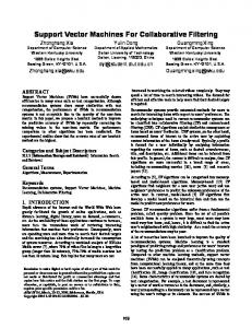
In Section 1.4.2, particular implementation details of a HOG/SVM based system are presented. This vision-based system, along with a Lidar sensor, is able to give spatial information about pedestrians in front of a vehicle. Histogram of Oriented Gradients. This feature has reached a maturity version for object matching in [1.21] and it was further modified by [1.10] to recognize pedestrians sequences. In Fig. 1.7, the feature is shown. It is composed by block descriptors, which, in turn, are formed by a set of cells, where the oriented gradients are accumulated. The size of the blocks and cells will determine how discriminative the recognition will be.

1. SVM and Features for Environment Perception

19

Fig. 1.7. Histogram of Oriented Gradients (HOG) is created by computing the values of the gradients (magnitude and orientation), as shown on left side of the picture. These values are accumulated into bins to form the histogram, right picture. The size of the histogram (size of the blocks and cells) will determine how discriminative the recognition will be.

In [1.21], the block descriptor is a set of 16×16 pixels. The oriented gradients, then, are obtained in a region of 4×4 pixels, which form the cell of the block descriptor. For each histogram, in each one of the 4 regions, there are 8 bins, computed around a full circle, i.e., each 45 degrees of orientation accumulates a value of the gradients. The blue circle, in Fig. 1.7, stands for a Gaussian function to weight each block descriptor, according to: 1 −(x2 +y2 )/2σ2 e . (1.59) 2πσ 2 where x and y are the coordinates of the centered pixel in the block descriptor window and σ is equal to one half of the width of the block descriptor window. The computation of the gradient at each point in the image I(x, y) is performed by calculating its magnitude m(x, y) and orientation θ(x, y), according to: G(x, y, σ) =

m(x, y) =

p

[I(x + 1, y) − I(x − 1, y)]2 + [I(x, y + 1) − I(x, y − 1)]2 . (1.60)

σ(x, y) = tan−1



I(x, y + 1) − I(x, y − 1) I(x + 1, y) − I(x − 1, y)



.

(1.61)

After the histograms are found, theyp are normalized by the L2-Hys norm, which corresponds to L2-norm, (v ← − v/ ||v||22 + ǫ2 ), followed by limiting the maximum values of v to 0.2, and renormalizing [1.21].

20

Rui Ara´ ujo et al.

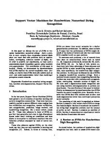
In [1.21], HOGs are just computed at stable points, i.e., partial rotation, translation and scale invariant points which are achieved by means of a pyramid of Gaussians. On the other hand, in [1.10], HOGs are computed over all image, densely. In the latter approach, HOGs are gathered through a normalized image window of predetermined size. Thereat, the input vector passed to a linear SVM has a constant size and represents an object/non-object decision. Haar Wavelet Templates. This kind of feature aims to describe regions with difference of color intensity. The name ‘Haar Wavelet’ indicates a particular discrete case of the wavelet transform. One of the first approaches using these features along with SVM can be found in [1.30] and further improved in [1.32]. These features have been represented by the following templates [1.32]:

Fig. 1.8. Wavelets templates: (a) vertical, (b) horizontal and (c) corner.

The templates shown in Fig. 1.8 come from the following equation:   1, γ(t) = −1,   0,

if 0 ≤ g < a, if a ≤ g < b, otherwise,

(1.62)

where g is a gray level intensity, and a and b correspond to the desired threshold. In [1.32], a set of wavelet templates have been collected over a 64×128 normalized image window for pedestrian detection, and submitted to an SVM of second degree polynomial kernel, according to:

f (x) = φ

N X i=1

αi yi (x.xi + 1)2 + b

!

(1.63)

where N is the number of support vectors and αi are Lagrange parameters. It is worthing notting that a number of new Haar wavelets features has been proposed and further utilized in [1.41] along with an Adaboost classifier. C2. Its creation was motivated by researches about how the brain of primate primary visual cortex works, which contains cells with the same name [1.36]. To extract the features, four stages are necessary:

1. SVM and Features for Environment Perception

21

– Application of a set of Gabor filters and elimination of those which are incompatible to biological cells. At the end, 8 bands are given to the next stage. This stage is called S1 and corresponds to simple cells in primate visual cortex; – Extraction of patches from the bands of previous stage (S1). – Obtaining S2 maps. – Computation of the max over all positions and scales for S2 maps. The output of this stage gives C2 maps which are scale invariants. In order to compute the bands for S1, a set of Gabor filters G(x, y, λ, θ, ψ, σ, γ) are applied to the input image:     ′2 x′ x + γy ′2 cos 2π + ψ . G(x, y, λ, θ, ψ, σ, γ) = exp − 2 ∗ σ2 λ

(1.64)

where x′ = xcosθ + ysinθ, y ′ = −xsinθ + ycosθ, θ represents the orientation of the normal to the parallel stripes function, ψ represents the offset of the phase, γ specifies the shape of the Gabor function support. In stage C1, after computing the final bands in the previous stage, patches are extracted in order to compose a set of ‘interesting points’ or ‘keypoints’. For all image patches (X) and each patch (P) learned during training, the following equation is applied so that S2 maps are obtained: Y = exp(−γ||X − Pi ||2 ) .

(1.65)

In the last stage, max(S2) over all positions and scales is computed and C2 features, which are scale invariants, are achieved. A study of C2 features is made in [1.36], where a linear SVM and a Gentle Adaboost are applied to classify the features, and similar classification results are reported.

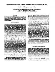
1.4 Applications 1.4.1 Learning to Label Environment Places This subsection describes a method for learning to classify places in indoor environments using SVM. The features presented in Sec. 1.3.1 are employed to the SVM classifier. The application method was performed on a embedded PC, located on-board of a robotic wheelchair (Fig. 1.9) [1.25]. The objective of the experiments is to demonstrate that the simple features presented in Section 1.3.1, used in conjunction with the SVM classifier presented in Section 1.2, can be used effectivelly to classify places. The results of the method will be later used as input to other methods such as the development of topological maps of the environment, localization, and improvement of human-robot communication.

22

Rui Ara´ ujo et al.

Fig. 1.9. Picture of the testbed robot (Robchair).

The global architecture of the method is presented at Fig. 1.10. Three distinct phases are involved in the operation of the method. In a first stage, data is gathered from the environment through a Lidar sensor. At a second stage, the raw Lidar data is processed into multiple features. Finally, the computed features are feed as inputs to the SVM classifier. The SVM classifier has two operation modes: the learning phase and the prediction phase (see section 1.2). Range data is collected using one Hokuyo URG-04LX Lidar [1.15] connected to the embedded computer through an Universal Serial Bus (USB). Range measurement scans are periodically acquired and post-processed into a collection of features for classification. The Hokuyo has a scanning range of 240 degrees. Each scan is composed of 632 range-bearing readings which are radially equally spaced by 0.36 degrees. Thus, each observation is z = {b1 , . . . , b632 }. Then each raw sensor range measure is used as input to the 15 feature extraction algorithms explained in Sec. 1.3.1. The outputs of the feature extraction algorithms are gathered into a fixed size vector. Thus, the feature mapping function is f : R632 → R15 . The next phase is the normalization of the feature vectors, with the objective of increasing the numerical stability of the SVM algorithm.

1. SVM and Features for Environment Perception

Raw

Laser Scan Data

Features Extraction Methods

Features Vector

23

Data Normalization

Operating Mode

SVM algorithm

(train/classify)

Output

Train

Classify

Fig. 1.10. Overall structure of the place classification system.

The sensor data sets were collected in the office-like building of ISRCoimbra (illustrated in Figure 1.11). The design of the method enables it to

Fig. 1.11. Map of the environment used in the experiments.

operate independently of specific environment characteristics (both in learning and prediction phases), i.e. the method is prepared to operate in various environments and to be robust to environment changes. In this context, five data sets were collected in several corridors and rooms. The first data set was used for training the classifier, and the other data sets were used to test the classification system with data representing new observation situations not present in the training data. The training data set was composed of 527 sensor observations zi and the corresponding place classifications υi . This is a relatively small training set. One of the four testing data sets corresponds

24

Rui Ara´ ujo et al.

to a corridor. The other three testing data sets were obtained in different rooms. In different training sessions, the SVM classifier was tested with three different kernels: sigmoid, polynomial of degree d = 5, and Gaussian RBF. After obtaining the SVM model, the classifier was tested with different data sets. Tables 1.2, 1.3, and 1.4 present the results obtained with the three different kernels. The best results were obtained with the Gaussian RBF kernel, where the hit ratio was always above 80%. These are promising results obtained with the relatively small data set used to train the SVM-based classifier. Table 1.2. Classification results for different indoor areas and using a sigmoid kernel

Corridor Lab. 7 Lab. 4 Lab. 5

Total samples

Correctly classified

Correct rate

48 112 27 57

36 84 18 43

75.00% 75.00% 66.67% 75.44%

Table 1.3. Classification results for different indoor areas and using a polynomial of degree d = 5 kernel

Corridor Lab. 7 Lab. 4 Lab. 5

Total samples

Correctly classified

Correct rate

48 112 27 57

38 88 21 43

79.16% 78.57% 77.78% 75.44%

Table 1.4. Classification results for different indoor areas and using a Gaussian RBF kernel

Corridor Lab. 7 Lab. 4 Lab. 5

Total samples

Correctly classified

Correct rate

48 112 27 57

41 92 22 44

85.42% 82.14% 81.48% 77.19%

1. SVM and Features for Environment Perception

25

The results show that place classification with SVM is possible with a high degree of confidence. The method can be extended by the introduction and testing of other kernels and additional features. 1.4.2 Recognizing Objects In Images As mentioned in Section 1.3, it does not usually suffice to use a raw input vector directly into a classifier, since this vector is not discriminative enough to capture certain aspects of data to separate object and non-objects through a consistent way. Hence, one usually need to find robust features to do the job. Motivated by [1.10], in this section, we explain our implementation details of a system to recognize and locate pedestrians in front of a vehicle. In Fig. 1.12, the framework of the system is illustrated. Firstly, the sensor data are acquired separately by using two different threads, one for the camera and the other for the Lidar. These threads communicate and are synchronized using shared memory and semaphores.

Fig. 1.12. Two threads are performed in the system: one responsible to the vision module and another one, responsible to Lidar segmentation. A rigid transformation are applied in order to map Lidar scanner space points to camera space points. At the end, the complete spatial location of the person in the image is given.

The module in charge of the Lidar scanner processing, then, segments the Lidar scanner points [1.5], as they arrive, and tries to cluster them, following the most probable hypothesis to be an object in the scene. Finally, this

26

Rui Ara´ ujo et al.

module transforms the coordinates of the world into image coordinates, by means of a rigid transformation matrix (see Fig. 1.13).

Fig. 1.13. A rigid transformation matrix is applied to transform world coordinates into image coordinates in order to give spatial information of the objects in the scene.

Concerning the image pattern recognition module, the algorithm proposed by [1.10] was implemented from scratch, with some slight modifications in order to speed up the classification process. The overall sketch of this method is described in Algorithm 1. Algorithm 1 Training and Classification of HOG / SVM Training stage - Extract feature vectors of normalized positive samples and random negative samples; - Normalize vectors; - Run classifier against negative samples, thoroughly; - Retrain hard examples; - Create final linear SVM model; Classification Stage - Scan images at different location and scale; - Predict classes with linear SVM model; - Fuse multiple detections; - Give object bounding boxes in image;

Firstly, a set of HOG features is extracted densely across the image. After feature normalization, feature vectors are passed to a linear SVM in order to obtain a support vector model. In case of negative features, which are

1. SVM and Features for Environment Perception

27

extracted randomly across non-object images, the model is retrained with an augmented set of hard examples to improve performance (bootingstrap strategy). The classification stage scans the input image over several orientations and scales through an image pyramid (see Fig. 1.14), all bounding boxes that overlap are clustered. For all stages, several parameters may be used and there exists a set of default optimal values [1.10].

Fig. 1.14. The input image is scanned over several orientations and scales through the image pyramid.

Fig. 1.14 illustrates the operation of Algorithm 1. Each level of the image pyramid is scanned by means of a sliding window. Afterwards, all the bounding boxes (red rectangle) are clustered with a non-maximum suppression algorithm (the blue path shows that the criterion to cluster the bounding boxes should be based on overlapping situations over the pyramid). Below, some more details are given concerning the classification tasks and sensor fusion, as well. Implementation Details. In our HOG/SVM implementation, the steps in Algorithm 1 were followed, except for two points: – the final bounding boxes were clustered not by means of a mean shift algorithm, but according to an area overlapping criterion: OA =

AL−1 ∩ AL ≥ 0.5 . AL ∪ AL−1

(1.66)

where AL−1 and AL represent the bounding boxes of the object in level L − 1 and L, respectively. – The maximum number of pyramid levels (Sn ) (see Fig. 1.14) is given by Eq. (1.67). However, it has been limited to 10 in order to decrease the computational cost.

28

Rui Ara´ ujo et al.

Sn = f loor



 log(Se /Ss ) +1 . log(Sr )

(1.67)

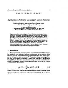
where Sr is the step constant, Ss is the initial step, equal to 1, and Se = min(Wi /Wn , Hi /Hn ), where Wi , Hi and Wn , Hn are the image size and positive normalized window size, respectively. Additionally, in order to obtain an improved classification speed, another implementation detail is worth to be realized. Since the algorithm proposed by Dalal and Triggs [1.10] presents high computational cost, we have decided to limit the classification region in the image by the Lidar Region of Interest (ROI), according to Fig. 1.13. In other words, the information that comes from the Lidar is used to establish as a focus of attention, narrowing the areas of the image that show more hypothesis to have a pedestrian. In Fig. 1.15, a snapshot illustrates results of the system. The output of the system is depicted in the image as different bounding box colors with the distance from the Lidar scanner, shown on the top of the bounding box. If the image pattern recognition module does not recognize the object as a pedestrian, only the Lidar works, giving the distance to the target. The system runs at 4 fps in a pentium M laptop, using linux.

Fig. 1.15. The output of the system is depicted in the image as different bounding boxes from the Lidar. Between 0 and 2 meters, the bounding box of the related object is red; between 2 and 4 meters, it is yellow, and beyond 4 meters, it is light blue.

As the system has been proposed to work as a pre-crash system, it was necessary to illustrates different distances from the object in front of the vehicle. Then, different colors highlight different levels of attention: 0 and 2 meters, the bound box of the related object is red, since the vehicle is very near from the object; between 2 and 4 meters, it is yellow, meaning that it is to have attention with the distance, and, finally, beyond 4 meters, it is

References

29

light blue, meaning that the object preserves a safe distance (all the criteria is based in a low speed vehicle). Linear SVM. Hitherto, nothing is known about the choice of linear SVM (Eq. 1.1) along with HOG features. In [1.10], a complete study shows the reason to use this type of SVM. After evaluating some kernels (polynomial and Gaussian), the linear SVM was chosen, since it was faster than the others kernelized SVM and has shown a better tradeoff between speed and classification performance. Although Gaussian kernel has shown the best classification curve. It is worth remembering that the generalization ability of SVM mainly relies on Eq. 1.20, since the smaller the number of support vectors concerning to the same number of training data sets, the better the generalization ability of the SVM.

1.5 Conclusions This chapter has presented SVM theory for learning classification tasks with some highlights of different features prone to work well with SVM. It has been also shown that it is possible to apply SVM for learning to semantically classify places in indoor environments to classify objects with good results. The proposed technique is based on training an SVM using a supervised learning approach, and features extracted from sensor data. The object recognition method was designed to improve the computational costs enabling the speed-up in operation which is an important factor for the application in real domains. The classification tasks employed a set of features extracted from Lidar and a vision camera. The good results attained with SVM encourage the development of new applications.

References 1.1 J. Almeida, A. Almeida, and R. Ara´ ujo: Tracking Multiple Moving Objects for Mobile Robotics Navigation, Proc. 10th IEEE International Conference on Emerging Technologies and Factory Automation (ETFA 2005), 2005 1.2 R. Ara´ ujo: Prune-Able Fuzzy ART Neural Architecture for Robot Map Learning and Navigation in Dynamic Environments, In: IEEE Transactions on Neural Networks, vol. 17, no. 5, pp 1235–1249, September, 2006. 1.3 G. Arnulf and B. Silvio: Normalization in Support Vector Machines, Proceedings of the 23rd DAGM-Symposium on Pattern Recognition, LNCS, SpringerVerlag, pp: 277–282, 2001 1.4 M. Bianchini, M. Gori, and M. Maggini: ”On the Problem of Local Minima in Recurrent Neural Networks,” IEEE Transaction on Neural Networks, Special Issue on Dynamic Recurrent Neural Networks, pp. 167–177, 1994. 1.5 G. Borges, and M. Aldon: Line Extraction in 2D Range Images for Mobile Robotics. Journal of Intelligent and Robotic Systems, v. 40, n. 3, pp. 267-297, 2004.

30

References

1.6 C. J. Burges, A Tutorial on Support Vector Machines for Pattern, Data Mining and Knowledge Discovery, Vol. 2, pp. 121-167, 1998. 1.7 J. Costa, F. Dias, R. Ara´ ujo: Simultaneous Localization and Map Building by Integrating a Cache of Features, Proc. 11th IEEE International Conference on Emerging Technologies and Factory Automation (ETFA 2006), 2006 1.8 N. Cristianini and J. Shawe-Taylor: An Introduction to Support Vector Machine and Other Kernel-based Learning Methods, Cambridge University Press, 2000. 1.9 K.-B. Duan1 and S. Sathiya Keerthi: Which Is the Best Multiclass SVM Method? An Empirical Study, In: N.C. Oza et al. (Eds.): MCS 2005, LNCS 3541, pp. 278-285, Springer-Verlag Berlin Heidelberg, 2005. 1.10 N. Dalal and B. Triggs: Histograms of Oriented Gradients for Human Detection. International Conference on Computer Vision and Pattern Recognition, 886–893, 2005. 1.11 R. Duda and P. Hart and D. Stork: Pattern Classification, Book News Inc., 2000. 1.12 R. Gonzalez, and R. Woods: Digital Image Processing, Addison-Wesley, 1993 1.13 I. Guyon and S. Gunn and M.Nikravesh and L. Zadeh: Feature Extraction: Foundations and Applications (Studies in Fuzziness and Soft Computing), Springer-Verlag, 2006. 1.14 H.S. Hippert, C.E. Pedreira, and R.C. Souza: Neural Networks for Short-term Load Forecasting: a Review and Evaluation. IEEE Trans. on Power Systems, v. 16, n. 1, pp. 44-55, 2001. 1.15 Hokuyo: Range-Finder Type Laser Scanner URG-04LX Specifications, Hokuyo Automatic Co., 2005 1.16 C. Hsu and C. Lin: A Comparison Methods for Multi-Class Support Vector Machine, In: IEEE Transactions on Neural Networks, vol. 13, pp 415–425, 2002. 1.17 T. Joachims: Optimizing Search Engines Using Clickthrough Data, Proceedings of the ACM Conference on Knowledge Discovery and Data Mining (KDD), ACM, 2002. 1.18 V. Kecman: Learning and Soft Computing, MIT Press, 2001. 1.19 H. Li, F. Qi, and S. Wang: A Comparison of Model Selection Methods for Multi-class Support Vector Machines, O. Gervasi et al. (Eds.): ICCSA 2005, LNCS 3483, pp. 1140-1148, Springer-Verlag Berlin Heidelberg, 2005. 1.20 S. Loncaric: A Survey of Shape Analysis Techniques, Pattern Recognition Journal, 1998 1.21 D. Lowe: Distinctive Image Features From Scale-invariant Keypoints. International Journal of Computer Vision, vol. 60, 91–110, 2004. 1.22 J. McInerney and K. Haines and S. Biafore and Hecht-Nielsen: Back Propagation Error Surfaces Can Have Local Minima. IJCNN., International Joint Conference on Neural Networks (IJCNN), 1989. 1.23 O.M. Mozos, C. Stachniss, A. Rottmann and W. Burgard: Using AdaBoost for Place Labeling and Topological Map Building, Robotics Research: Results of the 12th International Symposium ISRR, pp. 453-472, 2007 1.24 O. M. Mozos, C. Stachniss and W. Burgard: Supervised Learning of Places from Range Data Using Adaboost, In: IEEE International Conference Robotics and Automation, 742-1747, April, 2005 1.25 U. Nunes, J.A. Fonseca, L. Almeida, R. Ara´ ujo R. Maia: Using DisLaTeX Warning: There were multiply-defined labelstributed Systems in Real-Time Control of Autonomous Vehicles, In: ROBOTICA, Vol. 21, No. 3, pp. 271-281, Cambridge University Press, May-June, 2003. 1.26 Online. Acessed in: http://svmlight.joachims.org/ 1.27 Online. Acessed in: http://www.csie.ntu.edu.tw/~cjlin/libsvm/

References

31

1.28 Online. Acessed in: http://www.support-vector-machines.org/SVM soft.html 1.29 Online. Acessed in: http://www.kernel-machines.org/ 1.30 M. Oren and C. Papageorgiou and P. Shina and T. Poggio: Pedestrian Detection Using Wavelet Templates. IEEE Conference on Computer Vision and Pattern Recognition, 193–199, 1997 1.31 J. O’Rourke: Computational Geometry in C (Second Edition), Cambridge University Press, 1998. 1.32 C. Papageorgiou and T. Poggio: Trainable Pedestrian Detection. International Conference on Image Processing, vol. 4, 35–39, 1999 1.33 J. Platt: Using sparseness and analytic qp to speed training of support vector machines, Neural Information Processing Systems, 1999. Available: http://research.microsoft.com/users/jplatt/smo.html 1.34 C. Premebida, and U. Nunes: A Multi-Target Tracking and GMM-Classifier for Intelligent Vehicles, Proc. 9th IEEE Int. Conf. on Intelligent Transportation Systems, Toronto, Canada, 2006. 1.35 W. H. Press, S. A. Teukolsky, W. T. Vetterling, B. P. Flannery: Numerical Recipies (3 edition), Cambridge University Press, September 2007 1.36 T. Serre and L. Wolf and T. Poggio: Object Recognition With Features Inspired by Visual Cortex IEEE Conference on Computer Vision and Pattern Recognition, 994–1000, 2005 1.37 J. Shawe-Taylor and N. Cristianini: Kernel Methods for Pattern Analysis, Cambridge University Press, 2004. 1.38 A. Smola and B. Sch¨ olkopf. A Tutorial on Support Vector Regression, In: NeuroCOLT2 Technical Report NC2-TR, pp. 1998-2030, 1998. 1.39 C. Stachniss, O.M. Mozos, W. Burgard: Speeding-Up Multi-Robot Exploration by Considering Semantic Place Information, Proc. the IEEE Int.Conf.on Robotics & Automation (ICRA), Orlando, USA , 2006 1.40 S. Thrun, W. Burgard and D. Fox: Probabilistic Robotics, The MIT press,2005 1.41 P. Viola and M. Jones: Rapid Object Detection using a Boosted Cascade of Simple Features. IEEE Conference on Computer Vision and Pattern Recognition, 511–518, 2001 1.42 V. Vapnik: The Nature of Statistical Learning Theory, Springer Verlag, 1995. 1.43 A. Young: Handbook of Pattern Recognition and Image Processing, Academic press, 1986