division multiplexing in wireless communication, where multiple access to ..... of advantages over using time instants: (i) Guaranteed bounds on the local times at.
1
Time Synchronization and Calibration in Wireless Sensor Networks Kay R¨omer, Philipp Blum, Lennart Meier ETH Zurich, Switzerland
In this chapter, we review time synchronization and calibration for wireless sensor networks. We will first consider time synchronization in Sections 1.1–1.6, before turning to calibration in Section 1.7. We will show that time synchronization can be considered as a calibration problem and many observations about time synchronization can be transferred to calibration. In Section 1.1, we discuss applications of synchronized time in sensor networks, present challenges of sensor networks, and discuss why traditional synchronization approaches fail to meet these challenges. Section 1.2 presents models of sensor nodes, of hardware clocks, and of communication. Section 1.3 gives an overview of the various classes of synchronization. In Section 1.4, we present common synchronization techniques. Section 1.5 examines current synchronization algorithms. Section 1.6 presents common techniques for evaluating synchronization algorithms and selected evaluation results. 1.1
INTRODUCTION
Sensor networks are used to monitor real-world phenomena. For such monitoring applications, physical time often plays a crucial role. We will discuss these applications of time in Section 1.1.1. Providing synchronized physical time is a complex task due to various challenging characteristics of sensor networks. In Section 1.1.2, we present these challenges and discuss why synchronization algorithms for traditional distributed systems often do not meet these challenges.
i
ii
(b) (a)
(c)
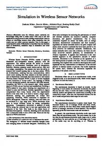
Fig. 1.1 Applications of physical time: (a) interaction of an external observer with the sensor network, (b) interaction among sensor nodes, and (c) interaction of the sensor network with the real world.
1.1.1
The need for synchronized time
Physical time plays a crucial role for many sensor-network applications. While many traditional applications of time also apply to sensor networks, we will focus here on areas specific to sensor networks. Figure 1.1 illustrates a rough classification of applications of physical time: (a) at the interface between the sensor network and an external observer, (b) among the nodes of the sensor network, and (c) at the interface between the sensor network and the observed physical world. The following paragraphs will discuss applications of time in these three domains. Note that some applications are hard to assign to a single domain. In such cases, we picked the most appropriate domain. Sensor network – observer In many applications, a sensor network interfaces to an external observer for tasking, reporting results, and management. This observer may be a human operator or an autonomous computing system. Tasking a sensor network often involves the specification of time windows of interest such as “only during the night”. As a sensor network reports observation results to an external observer, temporal properties of observed physical phenomena may be of interest. For example, the times of occurrence of physical events are often crucial for the observer to associate event reports with the originating physical events. Physical time is also crucial for determining properties such as speed or acceleration. Sensor network – real world In sensor networks, many sensor nodes may observe a single physical phenomenon. One of the key functions of a sensor network is hence the assembly of those distributed observations into a coherent estimate of the original phenomenon — this process is known as data fusion. Time is a key ingredient for data fusion. For example, if sensors can only detect the proximity of an object, then higher-level information (such as speed, size, or shape) can be obtained by correlating data from multiple sensor nodes. The velocity of a mobile object, for example, can be estimated by the quotient of the spatial and temporal distances between two consecutive sightings of the object by different sensor nodes. Since many instances of a physical phenomenon can occur within a short time, one of the tasks of a sensor network is the separation of sensor samples, that is
INTRODUCTION
iii
the partitioning of sensor samples into groups that each represent a single physical phenomenon. Temporal relationships (e.g., distance) among sensor samples are a key element for separation. Temporal coordination among sensor nodes may also be necessary to ensure correctness and consistency of distributed measurements [11]. For example, if the sampling rate of sensors is low compared to the frequency of an observed phenomenon, it may be necessary to ensure that sensor readout occurs concurrently at all sensor nodes in order to avoid false observation results (e.g., for calibration, see Section 1.7.5.2). It is anticipated that large-scale, complex actuation functions will be implemented by coordinated use of many simple actuator nodes. This requires temporal coordination. Within sensor network Time is also a valuable tool for intra-network coordination among different sensor nodes. Many applications of time known from traditional distributed systems also apply to wireless sensor networks. [17] points out a number of applications of time in distributed systems such as concurrency control (e.g., atomicity, mutual exclusion), security (e.g., authentication), data consistency (e.g., cache consistency, consistency of replicated data), and communication protocols (e.g., atmost-once message delivery). One particularly important example for concurrency control is the use of timedivision multiplexing in wireless communication, where multiple access to the shared communication medium is typically achieved by assigning time slots to the communicating nodes. This requires the participating sensor nodes to share a common view of physical time. A number of approaches intend to improve energy efficiency by frequently switching sensor nodes or components thereof into power-saving sleep modes (e.g., [35]). In order to nonetheless ensure seamless operation of the sensor network, temporal coordination of the sleep periods among sensor nodes may be required. Another important service for sensor-network applications is temporal message ordering (e.g., [28]). Many data-fusion algorithms have to process sensor readings ordered by the time of occurrence (e.g., the approach for velocity estimation sketched above). However, the highly variable message delays in sensor networks imply that messages from distributed sensor nodes may often not arrive at a receiver in the order in which they were sent. Reordering messages according to the time of sensor readout requires temporal coordination among sensor nodes. Methods for localization of sensor nodes based on the measurement of time of flight or difference of arrival time of certain signals do also require synchronized time (e.g., [13]). 1.1.2
Revisiting time synchronization for sensor networks
Time synchronization is a research area with a very long history. Over time, numerous algorithms have been proposed and have been in large-scale use. The Network Time Protocol (NTP) [21] is perhaps one of the most advanced and time-tested sys-
iv
tems. However, several unique characteristics of sensor networks often preclude the use of existing synchronization techniques in this domain. In the following, we discuss sensor-network challenges that impact the design of time-synchronization approaches. Using NTP as an example, we will outline why traditional approaches often do not meet the requirements of sensor networks (see also [9]). Note that some of the illustrated shortcomings of NTP are relatively easy to fix, while others are not. To provide the necessary background, we will first give an overview of NTP. NTP was designed for large-scale networks with a rather static topology (such as the Internet). Nodes are externally synchronized to a global reference time that is injected into the network at many places via a set of master nodes (so-called “stratum 1” servers). These master nodes are synchronized out of band, for example via GPS (which provides global time with a precision significantly below 1 µs). Nodes participating in NTP form a hierarchy: leaf nodes are called clients, inner nodes are called stratum L servers, where L is the level of the node in the hierarchy. The parents of each node must be specified in configuration files at each node. Nodes frequently exchange synchronization messages with their parents and use the obtained information to adjust their clocks by regularly incrementing them. Energy and other resources Sensor-network applications often require sensor nodes to be small and cheap. This has a number of important implications. First of all, the amount of energy that can be stored in or scavenged by small devices is typically very limited due to the low energy density of available and foreseeable technology. To ensure longevity despite this limited energy budget, energy-efficient design both in hardware and software becomes a dominating goal. Additionally, computing, storage, and communication capabilities of individual sensor nodes are rather limited due to size and energy constraints. These constraints may preclude the use of GPS or other technologies for out-ofband synchronization of NTP master nodes. NTP is also not optimized for energy efficiency, simply because this is not an issue in infrastructure-based distributed systems. Energy overhead in NTP results from several sources. Firstly, the service provided by NTP typically cannot be dynamically adapted to the varying needs of an application. Hence, with NTP all nodes would be continuously synchronized with maximum precision, even though only subsets of nodes might occasionally need synchronized time with less-than-maximum precision. Secondly, NTP uses the processor and the network in ways that would lead to significant overhead in energy expenditure in sensor networks. For example, NTP maintains a synchronized system clock by regularly adding small increments to the system-clock counter. This behavior precludes the processor from being switched to a power-saving idle mode. In addition, NTP servers must be prepared to receive synchronization requests at any point in time. However, constantly listening is an energywise costly operation in sensor networks; many sensor-network protocols therefore switch off the radio whenever possible.
INTRODUCTION
v
Network dynamics Due to their deployment in the physical environment, sensor networks are subject to a high degree of network dynamics. Sensor nodes can be mobile, die due to depleted batteries or due to environmental influences, and new sensor nodes may be added at any point in time. This results in relatively frequent and unpredictable changes in the network topology and possibly even in (temporary) network partitions. Mobile nodes can transport messages across partition boundaries by storing a received message and forwarding it as soon as a new partition is entered. The end-to-end delay of such message paths is very unstable and hard to predict. The operation of NTP is independent of the underlying physical network topology. In the NTP overlay hierarchy, a master and a client can be separated by many hops in the physical network, even though they are neighbors in the overlay hierarchy. Due to the above mentioned effects, multi-hop paths may be very unstable and unpredictable in a sensor network. NTP, however, depends on the ability to accurately estimate the delay characteristics of network links. NTP implicitly assumes that network nodes that shall be synchronized are a priori connected by the network. However, this assumption may not hold in dynamic sensor networks with mobile nodes. Consider for example an application where mobile sensor nodes with sporadic network connectivity time-stamp sensor readings and deliver these records to an observer as they pass by a base station (e.g., [15]). The base station may then want to compare time stamps generated by different sensor nodes in order to evaluate the collected data. However, in the above scenario, there might not be a network connection between the various originators of the time-stamped messages at any point in time. Hence, NTP cannot be applied in such settings. Infrastructure In many applications, sensor networks have to be deployed in remote, unexploited, or hostile regions. Sensor networks therefore often cannot rely on sophisticated hardware infrastructure. For example, under dense foliage or inside buildings, GPS cannot be used since there is no free line of sight to the GPS satellites. In order to improve the precision and availability of synchronization in large networks, NTP injects the reference time at many points into the network. Hence, any node in the network is likely to find a source of reference time in a distance of only a few hops. Note that shorter paths tend to be more reliable and more predictable, since they include fewer sources of error and unpredictability. However, such an approach requires an external infrastructure of reference-time sources which have to be synchronized with some out-of-band mechanism. Where this is not feasible, NTP would have to operate with a single master node, which uses its local time as the reference time. In large sensor networks, the average path length from a node to this single master is long, leading to reduced precision. This is particularly problematic when collocated sensor nodes require very precise mutual synchronization, for example to cooperate in observing a nearby physical event. With a single master node, the collocated nodes might end up using different synchronization paths, which results in different synchronization errors (i.e., time offsets) with respect to the master node.
vi
Configuration After initial deployment, it is often infeasible to physically access the sensor nodes for hardware or software maintenance. The large number of nodes also precludes manual configuration of individual nodes. While traditional networks such as the Internet do also consist of a large number of nodes, there is an accordingly large number of human network administrators, such that each one takes care of a manageable number of computers. With sensor networks, however, half a dozen of human operators may be responsible for thousands of sensor nodes. NTP requires the specification of one or more potential synchronization masters for each node. This is an appropriate solution for networks with a rather static topology, where configurations remain valid for extended periods of time. In sensor networks, however, network dynamics necessitate a frequent adaptation of configuration parameters. 1.2
SYSTEM MODEL
In the sections ahead we will analyze various synchronization approaches. We will now specify the system model for time synchronization that we use as the foundation of our analysis. First, we describe how we model clocks. We then specify the characteristics of communication between nodes in a sensor network. All our modeling is done in terms of discrete time and events. An event can represent communication between nodes, a sensor measurement, the injection of time information at a node, etc. We denote the real time at which event a occurs as ta , and the local time of node Ni at that time as hia . Note that our model does not explicitly contain node mobility or network dynamics; these aspects are included implicitly by the absence or existence of corresponding communication events. 1.2.1
Clock models
Digital clocks measure time intervals. They typically consist of a counter h (which we will also refer to as “the (local) clock”) that counts time steps of an ideally fixed length; we denote the reading of the counter at real time t as h(t). The counter is incremented by an oscillator with a rate (or frequency) f . The rate f at time t is given as the first derivative of h(t): f (t) = dh(t)/dt. An ideal clock would have rate 1 at all times, but the rate of a real clock fluctuates over time due to changes in supply voltage, temperature, etc. If the fluctuation were allowed to be arbitrary, the clock’s reading would obviously give no information at all. Fortunately, it is limited by known bounds. Different types of bounds on the rate fluctuation lead to different clock models: Constant-rate model The rate is assumed to be constant. This is reasonable if the required precision is small compared to the rate fluctuation.
SYSTEM MODEL
vii
Bounded-drift model The deviation of the rate from the standard rate 1 is assumed to be bounded. We call this deviation the clock’s drift ρ(t) = f (t) − 1 = dh(t)/dt − 1, and denote the corresponding bound with ρmax : −ρmax ≤ ρ(t) ≤ ρmax
∀t .
(1.1)
A reasonable additional assumption is ρi (t) > −1 for all times t. This means that a clock can never stop (ρi (t) = −1) or run backward (ρi (t) < −1). Thus, if two events a, b with ta < tb occur at a node Ni whose clock’s drift ρi is bounded according to (1.1), then node Ni can compute lower and upper bounds ∆li [a, b], ∆ui [a, b] on the real-time difference ∆[a, b] := tb − ta as: ∆li [a, b] :=
hi (tb ) − hi (ta ) 1 + ρmax
∆ui [a, b] :=
hi (tb ) − hi (ta ) . 1 − ρmax
(1.2)
This model is typically reasonable, since bounds on the oscillator’s rate are given by the hardware manufacturer. Sensor nodes usually contain non-expensive oscillators, and thus we have ρmax ∈ [10 ppm, 100 ppm]1 . Note that in this model, the drift can jump arbitrarily within the bounds specified in (1.1). The next model limits the variation of the drift. Bounded-drift-variation model The variation ϑ(t) = dρ(t)/dt of the clock drift is assumed to be bounded: −ϑmax ≤ ϑ(t) ≤ ϑmax
∀t .
(1.3)
This assumption is reasonable if the drift is influenced only by gradually changing conditions such as temperature or battery voltage. It makes drift compensation possible: A node can estimate its current drift and compute bounds on its drift for future times. We can also assume both (1.1) and (1.3). 1.2.2
Software clocks
A synchronization algorithm can either directly modify the local clock h or otherwise construct a software clock c. A software clock is a function taking a local clock value h(t) as input and transforming it to the time c(h(t)). This time is the final result of synchronization, and we therefore call it the synchronized time. For example, c(h(t)) = t0 + h(t) − h(t0 ) is a software clock that starts with the correct real time t0 and then runs with the same speed as the local clock h. In general, we require that a software clock is a piecewise continuous, strictly monotonically increasing function.
1 Parts per million, that is 10−6 . A clock with a drift of 100 ppm drifts 100 seconds in a million seconds, or 100µs in one second.
viii
1.2.3
Communication models
Communication is needed to obtain and maintain synchronization. In the following, we identify different communication parameters that affect time synchronization. Unicast vs. multicast If a message is sent by one network node and is received by at most one other network node, we call this unicast or point-to-point communication. Multicast communication occurs when a message is sent by one network node and is received by an arbitrary number of other network nodes. The case where all nodes within transmission range are recipients is called broadcast. Wireless sensor networks typically use simple broadcast radios, such that a sensor node’s transmission is overheard by all nodes within its transmission range. Symmetrical vs. asymmetrical links If we assume that node A can receive messages sent by node B if and only if node B can receive messages sent by node A, we say that the link between these two nodes is symmetrical. Otherwise, it is asymmetrical. An example for an asymmetrical link is the link between a base station with high transmit power and a mobile device with low transmit power: Beyond a certain distance between the two, only communication in direction from the base station to the mobile device is possible. In wireless sensor networks, it is reasonable to assume that there is a large number of small sensor nodes, and a small number of more powerful (regarding energy, memory, processing power, and transmit power) nodes. The links between these two types of nodes would clearly be asymmetrical. Implicit vs. explicit synchronization When comparing clock-synchronization approaches, it is important to distinguish whether synchronization information can be sent only with the messages that the sensor-network application transmits (“piggyback”), or whether additional communication (i.e., messages sent only for the sake of synchronization) is allowed. There is a trade-off between the amount of additional communication and the achievable synchronization quality. Additional communication incurs additional energy consumption and can reduce the bandwidth available for application data. Piggy-backed time information does typically not reduce bandwidth significantly, since there are no additional message headers to be transmitted or transmission slots to be occupied, and the time information is small in size. Delay uncertainty As far as synchronization is concerned, the goal of communication is to convey time information. The delay of the messages sent between nodes has to be taken into account when extracting this time information; we will explore this in Section 1.4.1. The message delay consists of
• the send time, lasting from when the application issues the send command to when the node actually starts trying to send; it is caused by kernel processing, context switches, and system calls, and hence varies with the current system load,
SYSTEM MODEL
ix
• the (medium) access time, lasting from when the node is ready to send to when it actually starts the transmission; this is the time that is spent waiting for access to the wireless channel, and hence depends on the current network load, • the propagation time, which is the time it takes for the radio signal to travel from the sender to the receiver; it is constant for any pair of nodes with constant distance, and is negligible compared to the other delay components in wireless sensor networks (since distances are small and radio signals travel very fast), and • the receive time, lasting from the reception of the signal to the arrival of the data at the application. The send and receive time (and especially the uncertainty about them) can be reduced by implementing the time-stamping of outgoing and incoming messages at a very low level, for instance in the MAC layer. As a general rule, message-delay uncertainties in typical wireless sensor networks are rather large compared to those in wired networks. This is due to the lower link reliability and bandwidth (see Section 1.1.2). 1.2.4
Sources of synchronization errors
Clock-synchronization algorithms face two problems: The information a node has about the local time of another node degrades over time due to clock drift (the two clocks “drift apart”), and its improvement through communication is hindered by message-delay uncertainty. The influence of drift and delay uncertainty on the quality of synchronization can to a large extent be studied separately. The influence of the clock drift may dominate over that of the message delays. This is the case in those sensor networks where communication is infrequent. The reason for this is that with decreasing frequency of communication, the uncertainty due to clock drift increases, while the uncertainty due to message delays remains constant. A numeric example: Suppose the message delay contributes 1 millisecond to a node’s uncertainty, and the clock drift is bounded by ρmax = 10 ppm. After 50 seconds, the drift’s contribution to the uncertainty equals that of the delay. After one hour, it is 72 times larger. In this setting, neglecting the delay uncertainty is acceptable. The time information that is obtained through communication has to be processed to achieve synchronization. As we will show in Sections 1.4.1 and 1.4.2, the computation power and memory size required to do this in a timely fashion can increase (even nonlinearly) with the amount of communication and thus become very large. There is a trade-off between computational power and storage capacity spent and achievable synchronization.
x
1.3
CLASSES OF SYNCHRONIZATION
Synchronization is commonly understood as “making clocks show the same time”, but there are actually many different types of synchronization. In the following, we will give an overview of the various choices available for synchronization. When choosing the synchronization approach for a given sensor-network application, the maxim is to fulfill the application’s requirements with the smallest possible effort in terms of computation, memory, and especially energy. 1.3.1
Internal vs. external
The synchronization of all clocks in the network to a time supplied from outside the network is referred to as external synchronization. NTP performs external synchronization, and so do sensor nodes synchronizing their clocks to a master node. Note that it makes no difference whether the source of the common system time is also a node in the network or not. Internal synchronization is the synchronization of all clocks in the network, without a predetermined master time. The only goal here is consistency among the network nodes. External synchronization requires consistency within the network and with respect to the externally provided system time. In everyday life, we are mostly faced with external synchronization, namely with keeping wristwatches and clocks in computers, cell phones, PDAs, cars, microwave ovens, etc. synchronized to the legal time. 1.3.2
Lifetime: continuous vs. on-demand
The lifetime of synchronization is the period of time during which synchronization is required to hold. If time synchronization is continuous, the network nodes strive to maintain synchronization (of a given quality) at all times. For some sensor-network applications, on-demand synchronization can be as good as continuous synchronization in terms of synchronization quality, but much more efficient. During the (possibly long) periods of time between events, no synchronization is needed, and communication and hence energy consumption can be kept at a minimum. As the time intervals between successive events become shorter, a break-even point is reached where continuous and on-demand synchronization perform equally well. There are two kinds of on-demand synchronization: Event-triggered on-demand synchronization is based on the idea that in order to time-stamp a sensor event, a sensor node needs a synchronized clock only immediately after the event has occurred. It can then compute the time-stamp for the moment in the recent past when the event occurred. Post-facto synchronization [8] is an example for event-triggered synchronization. We use time-triggered on-demand synchronization if we are interested in obtaining sensor data from multiple sensor nodes for a specific time. This means that there is no event that triggers the sensor nodes, but the nodes have to take a sample at precisely the right time. This can be achieved via immediate synchronization (where
CLASSES OF SYNCHRONIZATION
xi
sensor nodes receive the order to immediately take a sample and time-stamp it) or anticipated synchronization (where the order is to take the sample at some future time, the target time). Anticipated synchronization is necessary if it cannot be guaranteed that the order can be transmitted rapidly and simultaneously to all involved sensor nodes. This is especially the case if sensor nodes are more than one hop away from the node giving the order. Note that for successful anticipated synchronization, it is sufficient to maintain a synchronization quality which guarantees that the target time is not missed. This means that the required synchronization quality grows as the real time approaches the target time. There is no need to synchronize with maximum quality right from the beginning. Analogously to the event-triggered post-facto synchronization, we might refer to time-triggered synchronization as pre-facto synchronization. a)
b) N1
N2
N2
N3
N4
N5 Space
Scope N1
Lifetime
N3
N4 N5
Time
Scope
Fig. 1.2 Scope and lifetime define where and when synchronization is required. (a) shows the topology of some network, (b) illustrates scope and lifetime of the synchronization: Only nodes N2 , N3 and N4 need synchronization.
1.3.3
Scope: all nodes vs. subsets
The scope of synchronization defines which nodes in the network are required to be synchronized. Depending on the application, the scope comprises all or only a subset of the nodes. Event-triggered synchronization can be limited to the collocated subset of nodes which observe the event in question. 1.3.4
Rate synchronization vs. offset synchronization
Rate synchronization means that nodes measure identical time-interval lengths. In a scenario where sensor nodes measure the time between the appearance and disappearance of an object, rate synchronization is a sufficient and necessary condition for comparing the duration of the object’s presence within the sensor range of different nodes (but not for ordering the observations chronologically).
xii
Offset synchronization means that nodes measure identical points in time, that is at some time t, the software clocks of all nodes in the scope show t. Offset synchronization is needed for combining time stamps from different nodes. The difference between rate and offset synchronization is illustrated in Figure 1.3. Node N2 can compute the bird’s speed all by itself by dividing the distance between the bird’s positions at events a and b by the corresponding local-time difference. For this, the node’s clock must be rate-synchronized to the real-time rate 1. Alternatively, data from nodes N2 and N3 can be combined to compute the bird’s speed; here, we would use events b and c. The nodes’ clocks have to be offset-synchronized for this. a N2
b
c
N1
N3
Fig. 1.3 At events a, b, and c, nodes N2 and N3 measure the position of the bird and timestamp this data with their current local time. Rate or offset synchronization is needed depending on how the data from the three events is to be combined.
1.3.5
Timescale transformation vs. clock synchronization
Time synchronization can be achieved in two fundamentally different ways. We can synchronize clocks, that is make all clocks display the same time at any given moment. To achieve this, we have to perform rate and offset synchronization (or continuous offset synchronization, which however is costly in terms of energy and bandwidth and requires reliable communication links). The other approach is to transform timescales, that is to transform local times of one node into local times of another node. Both approaches are equal in the sense that if we have either perfect clock synchronization or perfect timescale transformation, the distributed sensor data can be combined as if it had been collected by a single node. The approaches differ in that clock synchronization requires either communication across the whole network (for internal synchronization) or some degree of global coordination (for external synchronization). This calls for communication over multiple hops (which however tends to degrade synchronization quality), or well-distributed infrastructure which for instance guarantees that every sensor node is only a few hops away from a node equipped with a GPS receiver. Timescale transformation does not have these drawbacks, but may instead incur additional computation and memory overhead. We illustrate the difference between clock synchronization and timescale transformation using the example shown in Figure 1.3. If the clocks of all three nodes are synchronized, node N1 can directly combine the sensor data from nodes N2 and N3 ,
SYNCHRONIZATION TECHNIQUES
xiii
since the time stamps refer to the same timescale. If the clocks are not synchronized, a timescale transformation on the received time stamps is necessary. The final result is identical to that of using synchronized clocks. 1.3.6
Time instants vs. time intervals
Time information can be given by specifying time instants (e.g., “t = 5”) or time intervals (“t ∈ [4.5, 5.5]”). In both cases, the time information can be refined by adding a statement about its quality. For instance, the time information may be guaranteed to be correct with a certain probability, or even probability distributions for the time can be given. A measure for the quality of the time information can then be defined; we will speak of its inverse, the time uncertainty. For sensor networks, the use of guaranteed time intervals can be very attractive. Interestingly, this approach has not received much attention, although it has a number of advantages over using time instants: (i) Guaranteed bounds on the local times at which sensor events occurred allow to obtain guaranteed bounds from sensor-data fusion. (ii) The concerted action (sensing, actuating, communicating) of several nodes at a predetermined time always succeeds: each node can minimize its uptime while guaranteeing its activity at the predetermined time. (iii) The combination of several bounds for a single local time is unambiguous and optimal, while the reasonable combination of time estimates requires additional information about the quality of the estimates. 1.4
SYNCHRONIZATION TECHNIQUES
In this section, building blocks and fundamental mechanisms of time synchronization algorithms are presented. The section is organized by increasing complexity: In Section 1.4.1, various approaches for obtaining a single reading of the clock of a remote node are presented. In Section 1.4.2, techniques for maintaining synchronization are discussed. In Sects. 1.4.3 and 1.4.4, it is shown how multiple samples can improve synchronization between two nodes. Finally, various approaches to organize the synchronization process in larger networks are discussed in Section 1.4.5. 1.4.1
Taking one sample
Assume the simple model shown in Figure 1.4 (a), with two nodes Ni and N j that can exchange messages. Synchronization between these nodes means that the nodes establish some relationship between their local clocks hi and h j . Unidirectional Synchronization The conceptionally simplest solution is illustrated in Figure 1.4 (b). Node Ni sends a message containing a local time stamp hia to node j N j , where it is received at local time hb . The node N j cannot determine the delay d of the message. It only knows that the local clock of node Ni showed hia before its own j j j local clock shows hb . Thus its local time when the message was sent is ha < hb , and
xiv
Ni Ni
hai Nj
d)
c)
b)
a)
hb
Nj
d
i
Ni
hb
h bi
Ni
h
d'
haj j
Nj j a
D
d
h ci
D
d1
Nj
d 1'
i
D
j
d2
h cj d 2'
h
i
h
j
h
i
h
j
h
i
h
j
Fig. 1.4 Uni- and bidirectional synchronization. a) A node N j determines the offset of its local clock relative to that of another node Ni , b) using unidirectional communication or c) and d) using bidirectional communication. In contrast to c), scheme d) allows both nodes to measure a round-trip time.
node Ni ’s local time when the message is received is hib > hia . Time synchronization j consists of estimating either hib or ha . If a-priori bounds on the message delay are known, that is dmin ≤ d ≤ dmax , then j j the estimation ha ≈ hb − 1/2(dmin + dmax ) (or alternatively hib ≈ hia + 1/2(dmin + j dmax )) minimizes the synchronization error in the worst case. Alternatively, hb −dmax j j and hb − dmin are lower and upper bounds on ha (and hia + dmin and hia + dmax are i bounds on hb ). Round-Trip Synchronization A slightly more complex solution is illustrated in Figure 1.4 (c). Node N j sends a query message to node Ni , asking for the time stamp j j hib . Node N j measures the round-trip time D = hc − ha , that is the length of the time interval between sending the request and receiving the reply. Without having a-priori knowledge, node N j now knows that the delay d is bounded by 0 and D. If a-priori bounds on the message delay are known, that is dmin ≤ d ≤ dmax , the node N j knows that d is bounded by max(D − dmax , dmin ) and min(dmax , D − dmin ). j j The estimation hb ≈ hc − D/2 minimizes the worst-case synchronization error; j j j hc − (D − dmin ) and hc − dmin are lower and upper bounds on hb . Similarly, an estii mation and bounds for hc can be determined. In comparison with the unidirectional approach, round-trip synchronization has the advantage of providing an upper bound on the synchronization error. The mechanism known as probabilistic time synchronization first presented in [5] uses this to decrease the synchronization error as follows: After receiving the reply message, N j checks whether the worst-case synchronization error D/2 − dmin is below a specified threshold. If not, it sends a new request message to Ni . This procedure is repeated until a pair of request and reply messages occurs that achieves the required synchronization error. The smaller the chosen threshold, the more messages have to be exchanged on average.
SYNCHRONIZATION TECHNIQUES
xv
The main disadvantage of round-trip synchronization is that the amount of messages increases linearly with the number of nodes that communicate with Ni , while in the unidirectional case, a single broadcast message sent by Ni can serve an arbitrary number of nodes. A combination of the advantages of both approaches is known as eavesdropping or anonymous synchronization and was first described in [7]. The basic idea is the following: Node N j sends a broadcast message to Ni and some additional node Nk , Ni replies with a broadcast message to N j and Nk . Node Nk assumes that the second message was produced after it had received the first message, thus node Nk can do round-trip synchronization with the two local receive time stamps and the send time stamp from Ni without ever producing any messages itself. In Figure 1.4 (d), two modifications of round-trip synchronization are illustrated. Firstly, it is not necessary that Ni replies immediately to query messages. Node Ni can instead measure the duration Di between receiving the query message and sending the reply, and the node N j can then account for this duration in its calculations. Secondly, the message exchange shown in Figure 1.4 (c) is asymmetrical, that is only N j can do round-trip synchronization. Therefore, at least one additional message from N j to Ni is required, such that also Ni can estimate or bound remote time stamps. Reference Broadcasting A third approach is shown in Figure 1.5. In addition to nodes Ni and N j , a so-called beacon node Nk is involved. The beacon sends a broadcast message to the other nodes. The delays d (to Ni ) and d 0 (to N j ) are almost equal. Ni then sends the time stamp hia to N j . Node N j measures the length of the time inj j terval D = hb − ha0 between the arrivals of the two messages and can then estimate hib ≈ hia + D. a)
b)
Ni
Nj
Nk
c)
Ni
Nj
Nk
Nk d
Ni
d'
hai Nj
ha'
d
hai
ha'
d'
ha'k D
j
D
h bi h
j
h bj
i
h
j
h
i
h
j
h
k
Fig. 1.5 Reference-broadcast synchronization. A node Ni determines the offset of its local clock relative to that of another node N j with the help of a third node Nk . In (c), a variant of reference-broadcast synchronization is shown that can be used if Ni and N j cannot directly communicate with each other (dashed link in (a)).
This approach was first proposed in [14] under the name a-posteriori agreement. It became more widely known in the sensor-network community as referencebroadcast synchronization (RBS) [8]. Its main advantage is that a broadcast message is received almost concurrently (even though its delay is largely variable), and thus
xvi
the synchronization error typically is smaller than with unidirectional or round-trip synchronization. The reference-broadcast technique can be used in many variations. For example, Figure 1.5 (c) shows a solution presented in [6] for the case that nodes Ni and N j , while being able to receive messages from Nk , cannot communicate with each other directly. N j replies to Nk , which then can estimate its own local time hka0 and send this information in another broadcast message to Ni and N j . In [8], yet another version is described: All nodes report their time stamps to a single node, which then broadcasts all information. The disadvantage of the reference broadcast approach is that physical broadcasts and a beacon node are required. 1.4.2
Synchronization in rounds
Typically, two local clocks do not run at exactly the same speed. Therefore time synchronization has to be refreshed periodically, the duration of the round depending on the error budget and the amount of relative drift between the two clocks. Let the length of a round be τround . Assume a round consists of a first period with length τsample , where one or more samples are taken according to one of the methods described in Section 1.4.1, and a second period where the nodes do nothing. Let us assume, that an application allows for a total error of Etotal , the maximum error after taking the samples is Esample , and the maximal drift rate is ρmax . Then the maximum length of a round τround has to satisfy τround ≤
Etotal − Esample . ρmax
The above relation implies that rounds can be longer if Esample and ρmax are small. For example, algorithms that use the round-trip technique can bound Esample according to the measured round-trip time and thus can dynamically increase τround if the roundtrip time was small. Other algorithms compensate the drift of the local clock and therefore can compute a smaller effective ρmax , which also allows to increase τround . In some applications, Etotal is smaller than what can be guaranteed by taking a single sample. In such a case, multiple samples can be taken to achieve Esample < Etotal . Taking multiple samples increases τsample . At the limit, τsample ≈ τround ; in this case, synchronization in rounds becomes a continuous process, rounds follow each other seamlessly. 1.4.3
Combining multiple time estimates
We now discuss techniques for combining multiple estimates of the local time of a remote node. Figure 1.6 (a) illustrates the situation: Every circle stands for a single j estimate of node N j ’s local time ha at some event a, which occurs at Ni ’s local time i ha .
SYNCHRONIZATION TECHNIQUES a)
h
xvii
b)
j
h
h
i
j
h
i
Fig. 1.6 Multiple samples improve on the synchronization error. (a) Every point represents a sample, that is a local time hi of node Ni and an estimated local time h j of node N j . Using interpolation techniques improves on the synchronization error. The solid line results from a linear regression on the samples, the dashed line is the result of a phase-locked loop (PLL). (b) The same idea can be used for lower (5) and upper (4) bounds on the local time of N j . Also here, interpolation can considerably improve on the synchronization error (i.e., on the uncertainty in this case). The solid lines are determined by the convex-hull approach, the dashed lines according to [30].
Linear Regression The most widely used technique is linear regression. A linear relation h j = α + β · hi is postulated and the coefficients α and β are determined by minimizing the square of the difference between the fitted h j ’s and the actual samples. This technique has a single parameter, that is the number of samples that are accounted for when computing the coefficients. A large number of samples can improve the regression quality, but requires a large amount of memory. The coefficient β can be interpreted as an estimation of h j ’s drift relative to hi . Linear regression thus implicitly compensates for clock drift. If the drift is variable, the postulated linear relationship between h j and hi does not describe reality very well. In such a situation, the number of samples accounted for should be small. The linear regression can be computed on-line, that is incrementally whenever a new sample is taken. An efficient on-line implementation can be found in [26]. A disadvantage of the linear-regression technique is that it weighs data points by the square of their error against the fitted line. Outliers thus have a particularly strong influence on the resulting coefficients α and β. Phase-Locked Loops Another method for processing a continuous sequence of samples is based on the principle of phase-locked loops (PLL) [12]. The PLL controls the slope of the interpolation using a proportional-integral (PI) controller. The output of a PI controller is the sum of a component that is proportional to the input and a component that is proportional to the integral of the input. The input of the controller is the difference between the actual sample and the interpolated value. If
xviii
the interpolation is smaller than the sample, its slope is increased, otherwise it is decreased. The main advantage of the PLL-based approach is that it requires far less memory than the linear-regression technique (in essence only the current state of the integrator sum). The main disadvantage is that PLLs require a long convergence time to achieve a stable rate [25]. The NTP algorithm uses a PLL [22]. 1.4.4
Combining multiple time intervals
The techniques of Section 1.4.1 can also be used to derive lower and upper bounds on the local time of a remote node. Figure 1.6 (b) shows a sequence of lower and upper bounds on the local times h j of a remote node N j on the y-axis and the corresponding local times hi of a node Ni on the x-axis. In the previous section, the samples formed a single cloud and the interpolation was a line “through the middle of this cloud”. Here we have two clouds, one formed by the lower-bound samples, the other by the upper-bound samples. The convex-hull technique [1, 36] interpolates the two clouds separately. One curve is drawn above all lower bounds, a second below all upper bounds. While linear-regression and PLL techniques tend towards the average of the individual samples, the convex-hull technique ignores average values and account for the samples with minimal or maximal error. This can result in improved robustness: While the current average message delay can be very unstable, the minimal message delay remains stable, though it may occur more or less frequently. In [30], it is proposed to interpolate lower- and upper-bound samples by a single line as follows: First the steepest and flattest lines that do not violate any lower or upper bound are determined. The slopes of these lines represent bounds on the drift of clock h j relative to hi . The “average”-line of these two extremal solutions is used as the final interpolation; for a more detailed description see Section 1.5.3. 1.4.5
Synchronization of multiple nodes
Sensor networks most often have a much more complicated topology than the simple examples shown in Figures 1.4 and 1.5, and not all sensor nodes can communicate with each other directly. Thus, multi-hop synchronization is required, which adds an additional layer of complexity. Clearly, this could be avoided by using an overlay network which provides virtual, single-hop communication from every sensor node to a single master node. But as we have seen in Section 1.4.1, the synchronization error directly depends on the message delay, which is very difficult to control on a logical link that is composed of many physical hops. Therefore, performant synchronization schemes have to deal with the multi-hop problem explicitly. Figure 1.7 illustrates various approaches to multi-hop synchronization. We now describe these four schemes and use them as examples to discuss the main problems of multi-hop synchronization. Out-of-band synchronization The conceptionally simplest solution is to avoid the problem: A large number of master nodes is distributed in the network such that every
SYNCHRONIZATION TECHNIQUES
a)
b)
c)
xix
d)
Fig. 1.7 Organizing synchronization in multi-hop networks. a) Single-hop synchronization with a set of master nodes which are synchronized out of band (e.g., using GPS). b) Single-hop synchronization in overlapping clusters, gateway nodes translate time stamps. c) Tree hierarchy with a single master node at the root. d) Unstructured.
node has a direct connection to at least one of these masters (e.g., [33]). The master nodes are synchronized among each other using some out-of-band mechanism. The global positioning system (GPS) is well suited to this purpose as it provides time information with sub-microsecond accuracy. However, GPS receivers are still relatively costly, consume a considerable amount of energy, and require a direct line of sight to a number of satellites and thus cannot operate inside buildings. Clustering The authors of the RBS algorithm propose to partition the network into clusters [8]. All nodes within a cluster can broadcast messages to all other members of the cluster and thus the reference-broadcast technique can be used to synchronize the cluster internally. Some nodes are members of several clusters and participate independently in all corresponding synchronization procedures. These nodes act as time gateways to translate time stamps from one cluster to the other. There is a tradeoff in choosing the size of the clusters. On the one hand, a small number of large clusters reduces the number of translations and thus improves the synchronization error; on the other hand, energy consumption grows quickly with increasing transmission range; this makes choosing many small clusters attractive. This trade-off has been examined in [23]. Tree Construction The most common solution of the multi-hop synchronization problem is to construct a synchronization tree with a single master at the root [10, 30, 32, 18]. Single-hop synchronization is applied along the edges of the tree. Various well-known algorithms can be used to construct such a tree [32]. As the accuracy degrades with the hop distance from the root, a tree with minimum depth is preferable. On the other hand, a small depth implies that the root has to serve many clients, and thus consumes far more energy than the other nodes. Tree construction faces two main problems: Firstly, in sensor networks, the network topology may be dynamic; nodes may be mobile and repeatedly join or leave the network. The multi-hop synchronization algorithms have to explicitly deal with such events. In particular, if the root node fails, a new root has to be elected [18]. Secondly, two neighboring (in terms of physical location) nodes may have a large
xx
hop distance in the synchronization tree. In consequence, the accuracy of synchronization between these nodes is not as good as if they would synchronize directly with each other. Unstructured As illustrated in the tree-construction approach, the multi-hop synchronization problem can be interpreted as the problem of determining the links and directions over which time information is disseminated. In contrast to treeconstruction approaches, unstructured approaches do not first explicitly solve this problem and then perform pairwise synchronization. Instead, time information is exchanged between any pair (or group) of nodes that communicate. Whereas in the tree-construction approach every pairwise synchronization is asymmetrical (i.e., between a client and a local master), it is symmetrical in the unstructured approach (i.e., between two equal peers). In [2], such an approach has been presented for intervalbased synchronization. Two nodes combine their bounds on real time by selecting the larger lower bound and the smaller upper bound. A similar approach for pointestimates is asynchronous diffusion proposed in [16]. Here, nodes that communicate adjust their synchronized clocks to the average of their synchronized times. Like the interval-based solution from [2], this approach is completely local. As these approaches do not maintain any global configuration, node mobility does not cause particular problems. In contrast, clustering and tree-construction schemes require that the global configuration has to be updated whenever nodes move or fail or when new nodes are added to the system. As algorithms that follow the unstructured approach do not attempt to communicate with a particular node (e.g., the parent node in a synchronization tree), some of these algorithms piggyback time stamps on messages that are sent for some other, not synchronization-related reason (e.g., [27, 2]). It could be argued that these algorithms have virtually no communication overhead, as no messages are generated exclusively for time synchronization. 1.5
CASE STUDIES
In the following subsections, we discuss a number of concrete synchronization algorithms from the literature (ordered by publication date). The goal here is to give an overview of the approaches (with reference to the techniques and classes discussed earlier in this chapter), rather than to discuss all the details. In addition, for each algorithm we will give some experimental results. Table 1.1 summarizes the underlying assumptions of the various protocols and classifies the approaches according to the criteria discussed in Section 1.3. 1.5.1
Time-stamp Synchronization (TSS)
TSS [27] provides internal synchronization on demand. Node clocks run unsynchronized, that is time stamps are valid only in the node that generated them. However, when a time stamp is sent to another node as part of a message, the time stamp is
CASE STUDIES
RBS
TPSN
TS/MS
LTS
TSS
IBS
TSync
FTSP
TDP
xxi
AD
Classes Internal vs. External
I
E
I
E
I
E
E
I
I
I
Cont. vs. On-demand
O
C
C
O
O
C
C
C
C
C
All nodes vs. Subsets
S
A
S
A/S
S
A
A
A
A
A
RO
O
RO
O
O
O
O
RO
O
O
Transform vs. Clocksync
T
C
–
C
T
C
C
C
C
C
Instants vs. Intervals
S
S
TS
S
T
T
S
S
S
S
X
X
X
X
X
X
X
X
X
X
X
X
X
Rate vs. Offset
Assumptions Broadcast Bidirectional communication
X
Constant rate
X
Bounded drift Multichannel MAC access
Table 1.1
X
X X
X
X
Synchronization classes and assumptions of time-synchronization protocols.
transformed to the timescale of the receiver. For messages sent over multiple hops, the transformation is repeated for each hop. Time-stamp transformation is achieved by determining the age of each time stamp from its creation to its arrival at a sensor node. On a multi-hop path, the age is updated at each hop. The time stamp can then be transformed to the receiver’s local timescale by subtracting the age from the time of arrival. The age of a time stamp consists of two components: (1) the total amount of time the time stamp resides in nodes on the path, and (2) the total amount of time needed to transfer the time stamp from node to node. The first component is measured using the local, unsynchronized clocks. The second component can be bounded by the round-trip time of the message and its acknowledgment. For the round-trip measurement, the technique depicted in Figure 1.4 (d) on page xiv is used, where the sender is Ni and the receiver is N j . Message d2 is a data message containing the time stamp, message d20 is an acknowledgment. Using the previous message exchange (d1 , d10 ), the receiver can use D j −Di as an upper bound for the delay of message d2 . If a minimum delay is known, it can be used as a lower bound (otherwise, 0 is used). Using storage time and the above bounds on transmission delay, lower and upper bounds of the time-stamp age can be determined. Additionally, ρmax is used to transform time intervals between node clocks as in (1.2) on page vii. With this approach, synchronization information is piggybacked to existing (acknowledged) messages. There are no additional synchronization messages, except when two nodes exchange a message for the first time. In this case, an additional initialization message must be sent and acknowledged in order to enable round-trip
xxii
measurement. An acknowledgment is not needed if the sender can overhear the receiver forwarding the message to the next hop, which is typically the case in broadcast networks. Measurements in a wired network with ρmax = 1 ppm showed that the average uncertainty of the time-stamp interval is about 200 µs for adjacent nodes. It increases by an additional 200 µs for each additional hop, and by about 2.5 µs per age second. 1.5.2
Reference-Broadcast Synchronization (RBS)
RBS [8] provides synchronization for a whole network. The basic synchronization primitive is a reference broadcast to a set of client nodes in the one-hop neighborhood of a beacon node as illustrated in Figure 1.5 (b) on page xv. The beacon node broadcasts manage synchronization pulses. The clients then exchange their respective reception times and use linear regression to compute relative offsets and rate differences to each other. Using offset and rate difference, each client can transform a local clock reading to the local timescale of any other client. To extend this scheme to multi-hop networks, the network is clustered such that a single beacon can synchronize all nodes in its cluster. Gateway nodes that participate in two or more clusters independently take part in the reference-broadcast procedure of all their clusters. By knowing offsets and rate differences to nodes in all adjacent clusters, gateway nodes can transform time stamps from one cluster to another. Time synchronization across multiple hops is then provided as follows. Nodes time-stamp sensor data using their local clocks. Whenever time stamps are exchanged among nodes, the time stamps are transformed to the receiver’s local time using offset and rate difference. In experiments it has been shown that adjacent Berkeley Motes can be synchronized with an average error of √ 11 µs by using 30 broadcasts. Over multiple hops, the average error grows with O( n), where n is the number of hops. 1.5.3 Tiny-Sync and Mini-Sync (TS/MS) Tiny-Sync and Mini-Sync [30] are methods for pairwise synchronization of sensor nodes. Both Tiny-Sync and Mini-Sync use multiple round-trip measurements and a line-fitting technique to obtain the offset and rate difference of the two nodes. For this, a constant-rate model (see page vi) is assumed. To obtain data points for line fitting, multiple round-trip synchronizations are performed as depicted in Figure 1.4 (c) on page xiv, where the client is N j and the reference is Ni . Each round-trip j j measurement results in a data point (hib , [ha , hc ]). Then, the line-fitting technique depicted in Figure 1.6 (b) on page xvii is used to calculate two lines with minimum and maximum slope. Slope and axis intercept of these two lines then give bounds for the relative offset and rate difference of the two nodes. The line with average slope and intercept of the two lines is then used as the offset and rate difference between the two nodes. Note that each of the two lines is unambiguously defined by two (a priori unknown) data points. The same results would be obtained if the remaining data points
CASE STUDIES
xxiii
could be eliminated. Since the computational and memory overhead depends on the number of data points, it is a good idea to remove as many data points as possible before the line fitting. Tiny-Sync and Mini-Sync only differ in this elimination step. Essentially, Tiny-Sync uses a heuristic to keep only two data points for each of the two lines. However, the selected points may not be the optimal ones. Mini-Sync uses a more complex approach to eliminate exactly those points that do not change the solution. Hence, Tiny-Sync achieves a slightly suboptimal solution with minimal overhead, Mini-Sync gives an optimal solution with increased overhead. Measurements on a 802.11b network with 5000 data points resulted in an offset bound of 945 µs (3230 µs) and a rate bound of 0.27 ppm (1.1 ppm) for adjacent nodes (nodes five hops away). 1.5.4
Lightweight Time Synchronization (LTS)
LTS [32] is a synchronization technique that provides a specified precision with little overhead, rather than striving for maximum precision as many other techniques. Two algorithms are proposed: one that operates on demand for nodes that actually need synchronization, and one that proactively synchronizes all nodes. Both algorithms assume the existence of one or more master nodes that are synchronized out-of-band to a reference time. The proactive algorithm proceeds by constructing spanning trees with the masters at the root by flooding the network. In a second phase, nodes synchronize to their parent in the tree by means of round-trip synchronization. The synchronization frequency is calculated from the requested precision, from the depth of the spanning tree, and from the drift bound ρmax . The on-demand version also assumes the existence of one or more master nodes. When a node needs synchronization, it sends a request to one of the masters using any routing algorithm (this is not further specified). Then, along the reverse path of the request message, nodes synchronize using round-trip measurements. The synchronization frequency is calculated as in the proactive version described above. In order to reduce synchronization overhead, each node may ask its neighbors for pending synchronization requests. If there are any such requests, the node synchronizes with the neighbor, rather than executing a multi-hop synchronization with a reference node. The overhead of the algorithms was examined in simulations with 500 nodes uniformly placed in a 120 m × 120 m area, a target precision of 0.5 s, and a duration of 10 hours. The centralized algorithm performed an average of 36 pairwise synchronizations per node. The distributed algorithm executed 4–5 synchronizations on average per node if 65% of all nodes request synchronization. 1.5.5
Timing-Sync Protocol for Sensor Networks (TPSN)
TPSN [10] provides synchronization for a whole network. First, a node is elected as a synchronization master (details for this are not specified), and a spanning tree with the master at the root is constructed by flooding the network. In a second phase, nodes synchronize to their parent in the tree by means of round-trip synchronization.
xxiv
Synchronization is performed in rounds and initiated by the root root broadcasting a synchronization-request message to its children. Each child then performs a round-trip measurement to synchronize with the root. Nodes further down in the tree overhear the messages of their parents and start synchronization when their parents have synchronized. To eliminate message-delay uncertainties, time-stamping for the round-trip synchronization is done in the MAC layer. In case of node failures and topology changes, master election and tree construction must be repeated. Measurements showed that two adjacent Berkeley Motes can be synchronized with an average error of 16.9 µs, which is a worse figure than the 11 µs given for RBS in [8]. However, the authors of [10] claim that a re-implementation of RBS on their hardware resulted in an average error of 29.1 µs between adjacent nodes, effectively claiming that TPSN is about twice as precise as RBS. 1.5.6
TSync
TSync [6] provides two protocols for external synchronization: the Hierarchy Referencing Time Synchronization Protocol (HRTS) for proactive synchronization of the whole network, and the Individual-Based Time Request Protocol (ITR) for ondemand synchronization of individual nodes. Both protocols use an independent radio channel for synchronization messages in order to avoid inaccuracies due to variable delays introduced by packet collisions. In addition, the existence of one or more master nodes with access to a reference time is assumed. With HRTS, a spanning tree with the master at the root is constructed. Then, the master uses the reference broadcasting technique illustrated in Figure 1.5 (c) on page xv to synchronize its children. Each child node now repeats the procedure for its subtree. Measurements in a network of MANTIS sensor nodes showed a mean synchronization error of 21.2 µs (29.5 µs) for two adjacent nodes (nodes three hops away). For comparison, RBS was also implemented, giving an average error of 20.3 µs (28.9 µs). 1.5.7
Interval-Based Synchronization (IBS)
Interval-based synchronization was first proposed in [19], where a bounded-drift model (see page vi) is assumed. The network nodes perform external synchronization by maintaining a lower and upper bound on the current time. During communication between two nodes, the bounds are exchanged and combined by choosing the larger lower and the smaller upper bound. This amounts to intersecting the time intervals defined by each pair of bounds. Between communications, each node advances its bounds according to the elapsed real time and the known drift bounds. In [29], the model was refined by including bounded drift variation and fault-tolerance. In [2], the simple approach from [19] was shown to be worst-case-optimal, where the worst case is the one where all clocks run with maximal drift. A considerable improvement in the synchronization quality can be achieved by having each node store, maintain, communicate, and use the bounds from its last communications with other
CASE STUDIES
xxv
nodes. In [20], it was shown that optimal interval-based synchronization can only be achieved by having nodes store and communicate their entire history. Obviously, this becomes prohibitive with growing network size and lifetime. In realistic settings, the value of a piece of history data decreases rapidly with its age. Therefore, efficient average-case-optimal synchronization can be obtained by using only recent data. 1.5.8
Flooding Time-Synchronization Protocol (FTSP)
FTSP [18] can be used to synchronize a whole network. The node with the lowest node ID is elected as a leader that serves as a source of reference time. If this node fails, then the node with the lowest ID in the remaining network is elected as the new leader. The leader periodically floods the network with a synchronization message that contains the leader’s current time. Nodes which have not received this message yet record the contained time stamp and the time of arrival, and broadcast the message to their neighbors after updating the time stamp. Time-stamping is performed in the MAC layer to minimize delay variability and hence uncertainty. Each node collects eight (time stamp, time of arrival) pairs and uses linear regression on these eight data points to estimate offset and rate difference to the leader. Measurements were performed in an eight-by-eight grid of Berkeley Motes, where each Mote has a direct radio link to its eight closest neighbors. With this setup, the network synchronized in 10 minutes to an average (maximum) synchronization error of 11.7 µs (38 µs), giving an average error of 1.7 µs per hop. 1.5.9
Asynchronous Diffusion (AD)
AD [16] supports the internal synchronization of a whole network. The algorithm is very simple: each node periodically sends a broadcast message to its neighbors, which reply with a message containing their current time. The receiver averages the received time stamps and broadcasts the average to the neighbors, which adopt this value as their new time. It is assumed that this sequence of operations is atomic, that is the averaging operations of the nodes must be properly sequenced. Simulations with a random network of 200 static nodes showed that the synchronization error decreases exponentially with the number of rounds. 1.5.10
Time Diffusion Synchronization (TDP)
TDP [31] supports the synchronization of a whole network. Initially, a set of master nodes is elected. For external synchronization, these nodes must have access to a global time. This is not required for internal synchronization, where masters are initially unsynchronized. Master nodes then broadcast a request message containing their current time, and all receivers send back a reply message. Using these round-trip measurements, a master node calculates and broadcasts the average message delay and standard deviation. Receiving nodes record these data for all leaders. Then, they turn themselves into so-called “diffused leaders” and repeat the procedure. The average delays and
xxvi
standard deviations are summed up along the path from the masters. The diffusion procedure stops at a given number of hops from the masters. All nodes have now received from one or more masters m the time hm at the initial leader, the accumulated message delay ∆m , and the accumulated standard deviation βm . A clock estimate is computed as ∑m ωm (hm + ∆m ), where the weights ωm are inversely proportional to the standard deviation βm . After all nodes have updated their clocks, new masters are elected and the procedure is repeated until all node clocks have converged to a common time. In a simulation with 200 static nodes with 802.11 radios and a delay of 5 seconds between consecutive synchronization rounds, the deviation of time across the network dropped to 0.6 seconds after about 200 seconds. 1.6
EVALUATION STRATEGIES
Evaluating the precision of time synchronization in wireless sensor networks is not a trivial task. For example, the authors of the RBS algorithm report 11 µs precision on the Berkeley Motes platform [8], while the authors of the TPSN algorithm report 29 µs for RBS on the same platform, concluding that TPSN is better, as it achieves 17 µs [10]. Which numbers are correct? Probably all of them, but the evaluation was done slightly differently. In this section, we discuss different evaluation strategies that have been applied to time-synchronization algorithms for wireless sensor networks. There are various aspects of the performance achieved by an algorithm than can be evaluated, for example the energy consumption or the message and memory overhead. The discussion in this section concentrates on various alternatives for the evaluation of the precision of time-synchronization algorithms. 1.6.1
What is precision?
Figure 1.2 (b) on page xi illustrates the scope and lifetime of synchronization in a sensor network. The scope defines which nodes have to be synchronized and the lifetime defines when these nodes have to be synchronized. Thus it is natural to evaluate the precision in the shaded area of Figure 1.2 (b). The precision is a metric that is closely related to the synchronization error. While the precision is a single scalar value for a whole network, the synchronization error is a function of time for a single node. In the following, we discuss several alternatives to map such functions to a single scalar precision value P. Combining the synchronization error of many nodes At some time t within the lifetime of a sensor network, every node Ni within the scope has a synchronized time ci (hi (t)). In the case of internal synchronization, the instantaneous precision p(t) is
EVALUATION STRATEGIES
xxvii
often defined as the maximal difference between any two synchronized times, that is � p(t) = max ci (hi (t)) − c j (h j (t)) i, j
for any nodes Ni and N j within the scope. Some authors (e.g., [31]) use the standard deviation among all ci (hi (t)) as a measure for the instantaneous precision at time t. In the case of external synchronization, the instantaneous precision is more often defined as the maximal synchronization error, that is � p(t) = max ci (hi (t)) − t i
for any node Ni within the scope. This variant of precision is sometimes called accuracy. Alternatively, the precision can be defined as the average synchronization error within the scope or the maximal synchronization error among the 90% (or 99%, etc.) nodes in the scope with the smallest synchronization error. Steady State and Convergence Time The instantaneous precision p(t) obviously varies during the synchronization lifetime. The final precision metric P can be derived by taking the maximum of p(t) for all t in the lifetime. Alternatively, the average of p(t) can be used. It is clear that the precision P improves in proportion to the time the synchronization process is active, and that at some point, the improvement stops. Usually, the precision P is evaluated after this point, that is the lifetime of synchronization starts after the synchronization process, and the precision P describes the steady state. Some authors evaluate the convergence time, which is the length of the interval from the start of the synchronization process to the point in time where the precision P stops to improve or reaches a specific value. If the lifetime is defined, the convergence time indicates when the synchronization process has to be started such that the desired precision P is achieved before the start of the lifetime and is maintained until the end of the lifetime. 1.6.2
Goals of performance evaluation
There can be different reasons why the performance of an algorithm has to be evaluated, and different goals lead to different solutions. The actual performance of a given synchronization algorithm strongly depends on properties of the target platform. It is difficult to identify and model all the influence factors explicitly. A realistic estimation of the achievable precision is thus best obtained by using measurements on the actual target platform, rather than using simulation of a simplified target platform. Sometimes, realistic estimation of the performance is less important than fairness and repeatability of the evaluation. This is the case if several competing algorithms have to be compared. Also in the optimization process of the parameters of a particular algorithm, it is important that differences in the performance are due to differences in the algorithm and not due to different conditions (e.g., message delays, clock
xxviii
drift). Here, simulation based on recorded or generated traces is more appropriate than direct measurements. If the goal of analyzing a particular synchronization algorithm is to give worstcase guarantees on its performance, neither measurements nor simulation based on recorded traces can be used, since both strategies only evaluate a finite number of instances. Instead, the worst-case has to be identified and the worst-case performance has to be determined analytically. 1.6.3
Measurements
Measurement techniques Three fundamentally different measurement strategies, which are illustrated in Figure 1.8, have been used in recent publications. a)
b)
Log File
c)
Log File
Analyzer Log File
out-of-band synchronization
Log File
Log File virtual nodes on a single physical node
generate events
Fig. 1.8 Precision-measurement techniques. a) Every node is synchronized out of band and measures its own precision. b) Every node generates events, the evaluation is centralized. c) Some nodes are virtual nodes on the same hardware platform as the master node.
Consider Figure 1.8 (a). Every sensor node executes two synchronization procedures, synchronizing two different clocks. The first procedure is the actual synchronization algorithm under test, using only the means of the platform on which it is executed. The second procedure is another algorithm, which achieves a far better precision than the first. This is possible since this second synchronization uses resources that are not offered by the target platform, but which are introduced for the measurements. A GPS receiver for every sensor node can serve this purpose. Alternatively, cable connections can be used as an out-of-band mechanism with very low delay variability to provide a reference time (e.g., [24], [8], [3]). In [18], a singlehop RBS scheme is used to measure the precision achieved by the FTSP multi-hop algorithm. This approach has the advantage that every node can evaluate and log its own precision and these values can be collected at the end of the experiment (or even on-line), providing complete information. An alternative is shown in Figure 1.8 (b). All sensor nodes generate some directly observable event, for example a rising edge on a particular I/O pin, when their synchronized time reaches a particular value X. An external analyzer device then records the time interval between the instance when a node’s synchronized time is X and the instance when it really is X. Such a procedure has been used for example in [10]. Its
EVALUATION STRATEGIES
xxix
advantage is that the precision of the measurement is not limited by the resolution of the nodes’ clocks or the performance of a second synchronization procedure. As illustrated in Figure 1.8 (c), [27] proposes to measure the precision achieved by one client node as follows: A client node synchronizes over several hops to a master node. Master and client nodes are virtual nodes emulated on a single physical node, the intermediate nodes are all separate physical nodes. As the master and the client share a single hardware clock, the precision of the client can easily be evaluated. Systems and Topologies All three approaches do not scale well. Therefore, only small networks have been used so far for measurements. The largest experiment is described in [18], where a 8-by-7 grid of Mica2 Motes is evaluated. In [10], a chain of 6 Mica Motes is used, [6] evaluates 5 MANTIS Nymph nodes, [27] evaluates a chain of 7 standard PCs with 100 Mbit/s wired Ethernet, and [8] evaluates IPAQ nodes communicating over 802.11b WLAN and Mica Motes. How the synchronization error of hundreds of nodes should be measured is an open question. Current evaluations of such large networks are all based on simulation. Results We will now give some measurement results from recent publications. Our intention is to give an idea about the order of magnitude of the achievable precision and to illustrate that although all results are about precision, they are difficult to compare. In [18], the convergence time of the FTSP algorithm in a 7-by-8 grid is reported to be 10 minutes. A maximal error of 38 µs and an average error (over all nodes) of 12 µs is reported. For the TPSN algorithm, [10] reports a maximal error of 45 µs for one hop and 74 µs for five hops. Average errors (over time) are 17 µs for one hop and 38 µs for five hops. The authors provide also the percentage of the time when the synchronization error was below the average error (> 60%). The authors of RBS present in [8] the distribution of the synchronization error (over time) for one hop and the mean, median, 95% and 99% values over 300 trials for one to four hops. Some authors evaluate the distribution of the synchronization quality in the system. At some time t, either the synchronized times ci (hi (t)) of all nodes i [31], or alternatively the corresponding synchronization errors ei (t) [10, 6], are shown in a histogram. 1.6.4
Simulation
Performance evaluation through simulation has the advantage that the resulting precision or accuracy of all nodes does not have to be measured but is directly accessible. Thus, much larger systems can be evaluated. Systems and Topologies In [31], systems with 200 nodes are evaluated, in [16] and [32] up to 500 nodes, always randomly placed in a square area. The transmission range of the nodes is 10 m in a square of length 80 m [31] or 120 m [32]; in [16], various transmission ranges from 0.4 m to 1 m are used in a square of length 10 m.
xxx
In [2], the transmission range is varied between 0.1 and 0.5 times the width of the square area. In [30], a chain of 5 nodes is simulated. Message Delays For simulation, a number of assumptions about the behavior of the system have to be made (e.g., about message delays). In [30], measured delay traces from an 802.11 wireless LAN are used, [31] and [32] generate delay traces according to a normal distribution. In [31], an additional offset is added which increases when the medium is saturated, that is when more than 75% of the channel capacity is used. The authors of [2] assume zero message delay, arguing that the synchronization errors induced by delay uncertainty and drift can be studied separately. Clock Drift In [31] and [2], every node is assigned an arbitrary but constant drift rate between −100 ppm and +100 ppm. In [32], all nodes have a drift rate of 50 ppm. Results The main concern of [32] is to compare centralized and distributed versions of the LTS algorithm in terms of required messages and achieved synchronization error. The average error (over all nodes) is evaluated as a function of the hop distance to the master node. [30] evaluates the synchronization error and the drift-compensation error achieved by the TS/MS algorithms as a function of time. A node one hop away from the master has an error of 1 ms after 83 minutes. A node with five hops distance achieves 3 ms. In [2], the average synchronization error (over time and over all nodes) is evaluated as a function of the number of messages exchanged between the nodes. Also the impact of the transmission range and of the number of master nodes is evaluated. The authors of [16] mainly evaluate how quickly (number of rounds) a network synchronizes using the AD algorithm. This is evaluated as a function of the transmission range and as a function of the number of nodes in the system. It is also shown that the synchronization error decreases exponentially with the number of rounds. The speed of convergence is also evaluated in [31], here for the TDP and TPSN algorithms; the standard deviation of the nodes’ synchronization error is shown as a function of time. It is argued that node mobility makes convergence slower. In addition, histograms and three-dimensional plots of the distribution of the synchronization error after convergence are presented. 1.6.5
Challenges of a benchmark
So far, we have presented how synchronization algorithms are evaluated in current literature. We have seen that results of different authors are quite incomparable due to widely differing goals, assumptions and techniques. On the one hand, there is not yet a common understanding about the requirements on synchronization in sensor networks. On the other hand, there is also disagreement about available resources and platforms. A benchmark for comparing the various algorithms on common grounds has not yet been presented. In the following, we discuss why it is difficult to devise a benchmark that can be used with a large number of algorithms. Ideally, the comparison of algorithms is based on simulation using system traces. Such traces should contain
CALIBRATION
xxxi
the system and communication model (How many nodes are there? How many of them are master nodes? Which node communicates with which other node at which time?), and they should characterize the “adversary” of synchronization, namely all message delays and the drift rates of the nodes. But this would require to determine all communications before executing the algorithms. This is not possible for most of the algorithms, since they actively decide to generate messages, depending on previous events. Furthermore, some algorithms require broadcast communication, while others do not. 1.7
CALIBRATION
In the previous sections, we have considered the problem of time synchronization, where the output of a hardware clock had to be mapped to a timescale. Sensor calibration is the problem of mapping the output of a sensor to a well-defined scale. In this section, we want to take a step back from time synchronization and consider the more general problem of calibration. As we will show, there is a close relationship between calibration and time synchronization, since the latter can be considered a special case of the former. It might be somewhat unfamiliar to consider a hardware clock as a sensor, but we will as show in Section 1.7.1 that the difference is rather subtle. The remainder of this section is structured in a similar way as the discussion of time synchronization in the previous sections. Section 1.7.2 explains why new approaches are required for calibration in sensor networks. Section 1.7.3 presents our system model for sensors. Section 1.7.4 discusses various classes of calibration. Section 1.7.5 presents concrete calibration algorithms from current literature. 1.7.1
Time synchronization as calibration
Sensors are hardware devices that have an input and an output. The input is a certain physical quantity in the real world, such as temperature, light intensity, acceleration, radio signal strength, etc. The output typically is a variable electrical signal such as a voltage or current. An analog-to-digital converter converts it to a digital number. A hardware clock typically consists of four components: a physical system that has a periodic behavior (e.g., an oscillating quartz, decaying Cesium, a pendulum), a sensor that converts the physical phenomenon to an electrical signal, an analog-todigital converter (e.g., threshold detector) that converts the output of the sensor to a one-bit number, and a counter that counts the number of rising (or falling) edges seen so far in the digital output stream. Hence, a hardware clock contains, among other things, a sensor and the physical phenomenon to observe. Despite this analogy, time as a physical quantity has some unique characteristics. For example, in many practical settings, observed physical quantities have a rather limited range of values (e.g., temperature ∈ [−30◦C, +30◦C]). Given a bounded relative sensor error (i.e., bounded drift), the absolute measurement error is then also bounded. However, physical time eventually grows beyond all bounds. Hence, the absolute error of a software clock is unbounded unless synchronization messages are
xxxii
exchanged. This explains the need for precise drift compensation and for repeating synchronization after a certain amount of time. 1.7.2
Revisiting calibration for sensor networks
Calibration is a very old problem, since it is needed for almost all measurement instruments. Despite this, calibration in sensor networks has so far not received much attention by researchers — at least when compared to time synchronization. However, a number of challenges to calibration in sensor networks pose interesting questions. A large number of sensor nodes often cannot be calibrated manually and individually. This is particularly true for pairwise calibration, where a sensor measures a quantity emitted by another device (i.e., an actuator). One example for this is measuring the radio signal strength to infer the distance between devices. In such a scenario, every sensor would have to be calibrated against every transmitter, resulting in a quadratic number of calibration steps. Sensors may be exposed to significant changes of environmental parameters (e.g., temperature, humidity) during the lifetime of a sensor network. Since the commonly used low-cost sensors are rather sensitive to such changes, a one-time factory calibration may not be sufficient. In this case, periodical calibration during the lifetime of the sensor network is necessary. 1.7.3
System model
The physical quantity q that is observed by a sensor is mainly a function of the size of the sensor, of its orientation, of its location, and of time t. Since the size of a sensor is non-zero, sensors can typically only observe the accumulation (e.g., weighted average) of a physical quantity over a certain area or volume. If we assume that size, orientation, and location are constant properties of a sensor i, we can denote the time-dependent physical quantity observed by the sensor as qi (t). Often, q is a real-valued scalar function (e.g., for temperature sensors), but may also be more complex (e.g., for a location sensor, q might return triples (x, y, z)). The output of a sensor i under stimulus qi (t) is denoted as hi (t). Note that hi (t) for a given qi (t) typically depends on a number of parameters, for example fabrication tolerance of the sensor, environmental parameters such as temperature and humidity, and wear of the sensor. In analogy to software clocks, we introduce a software sensor as a function c that maps a sensor output h(t) to c(h(t)). Software sensors are typically introduced to map a sensor output to a standard scale (e.g., the Celsius scale). Here, the goal of calibration is to find a suitable c for a given scale. Often, q does refer to such a standard scale, in which case the goal of calibration could be to find a c which approximates ci (hi (t)) = qi (t) for all t. As mentioned in the previous section, calibration may also be applied to actuators. An actuator can be considered a reverse sensor that accepts a digital value h(t) as input and produces a physical quantity q(t) as output. For example, a heater may
CALIBRATION
xxxiii
accept a temperature specification as input and heat until this temperature is reached. A software actuator c−1 then maps a given value v to c−1 (v), which may be used as an input to the actuator to produce a certain physical quantity (e.g., such that q(t) = v). 1.7.4
Classes of calibration
In this section, we adapt the classes of time synchronization introduced in Section 1.3 to calibration. Internal vs. external For internal calibration, all software sensors i should output the same value ci (hi (t)) if they are exposed to an identical stimulus q(t) (note that if for instance q(t) = 25◦ C, then c1 (h1 (t)) = c2 (h2 (t)) = 10◦ C would mean that sensors 1 and 2 are internally calibrated). For external calibration, the output of all software sensors must conform to a specified scale (e.g., if q(t) = 25◦ C, then c1 (h1 (t)) = c2 (h2 (t)) = 25◦ C is required). Lifetime: continuous vs. on-demand As some of the parameters that influence h may change over time, calibration may have to be repeated to adapt to these parameters. Calibration may be performed continuously or on demand. Scope: all nodes vs. subsets All nodes or only subsets of nodes might participate in calibration. For example, only some nodes might be equipped with a certain type of sensor, or the sensor might only be used by some nodes. Rate vs. offset Sometimes it is sufficient if differences ci (hi (t1 )) − ci (hi (t2 )) (e.g., temperature differences) obtained from different sensor instances can be compared. In this case, rate calibration is sufficient. If, however, absolute values ci (hi (t)) (e.g., absolute temperature values) originating from different sensor nodes are to be compared, offset calibration is needed. Scale transformation vs. global scale Rather than having all software sensors adhere to a global scale, it might be advantageous (e.g., in terms of overhead) to maintain local scales and transform sensor readings as they are sent to nodes with a different scale (e.g., if node 1 uses the Celsius scale and node 2 uses the Fahrenheit scale, then the transformation function for transforming from node 1 to node 2 is c12 (h1 (t)) = 1.8h1 (t) + 32). Point estimates vs. bounds Software sensors may either output point estimates (in analogy to time instants for time synchronization) or bounds (in analogy to intervals for time synchronization).
xxxiv
1.7.5
Case studies
In this section, we present two calibration algorithms for sensor networks (ordered by publication date). As in Section 1.5, we outline the algorithm and give an idea of its performance. 1.7.5.1 Calibration as Parameter Estimation (CPE) Calibration as Parameter Estimation [34] provides a framework for external calibration where sensors measure a quantity emitted by an actuator. Both the behavior of the actuator and of the sensor are unknown and must be taken into account for calibration. The general approach here is the joint calibration of sensors and actuators such that the overall system response is optimized. The algorithm will be illustrated by pairwise distance measurements between sensor nodes using the time of flight of an ultrasound signal. Each node is equipped with a speaker (the actuator) and a microphone (the sensor). Assuming the nodes have synchronized clocks, one node emits an acoustic signal containing a time stamp, the other receives the acoustic signal, computes the time of flight, and it multiplies with the speed of sound to obtain a distance estimate. For our discussion, we will consider a virtual distance sensor that directly outputs a distance estimate h(t) given the true distance as the physical stimulus q(t). Due to reasons discussed below, distance estimates include various systematic errors. Hence, the goal of calibration is to find a function c that maps the distance estimate h(t) to the correct distance q(t). For CPE, c must now be parameterized, such that it is expressed as a function of h and of parameters that describe the various error sources. These parameters are related to both the sensor and to the actuator. For example, the distance h(t) output by the sensor can be expressed in terms of the true distance q(t) as follows: h(t) = BT + BR + GT q(t) + GR q(t) where BT and BR refer to constant distance offsets caused by startup times for diaphragm oscillation in the transmitter and in the receiver, respectively; GT and GR represent the distance-dependent influence of the transmitter volume and of the receiver sensitivity, respectively. Solving for c(h(t)) := q(t) we obtain: c(h(t)) = (h(t) − BT − BR )/(GT + GR ) Although there is one instance of the above joint-calibration function for every transmitter–receiver pair, there is only one set of parameters (BT , BR , GT , GR ) for each of the N nodes. Hence, we can formulate a linear equation system with 4N variables (i.e., the four above parameters for each node) and 4N equations, which requires 4N pairs (h(t), c(h(t)) = q(t)) to solve. Alternatively, more samples can be collected and least-squares optimization can be used to obtain more accurate estimates for the parameters. Once the parameters (BT , BR , GT , GR ) for each node are known, the calibration functions are also known.
CALIBRATION
xxxv
The authors performed an experiment with an 8 × 4 square grid of Berkeley Motes with a node distance of 30cm, such that the true distances between pairs of nodes can be easily calculated. Each node emitted an ultrasound beacon, which allows all other nodes to estimate their distance to the transmitting node. The average error of the uncalibrated distance estimates is 74.6%. With the above calibration procedure, the average error could be reduced to 10.1%. 1.7.5.2 Collaborative In-Place Calibration (CIC) CIC [4] supports internal calibration under a number of assumptions: the sensor nodes should be densely deployed, sensor orientation should have a negligible impact on the sensor output, spatial frequency of the observed physical quantity should be low, temporal frequency of the quantity should be high. Essentially, these assumptions ensure that collocated sensor nodes will see very similar stimuli q(t) that change quickly over time. Additionally, it is assumed that q, h, c are real-valued, scalar functions. Calibration functions c are assumed to be linear functions, although the method could also be adapted to non-linear functions. The algorithm consists of two phases. In the first phase, pairwise calibration among collocated nodes is performed. In the second phase, calibration among remote nodes is performed. In the first phase, collocated pairs of nodes are calibrated against each other. Let us assume node 1 has to be calibrated against node 2. Then the goal is to derive a linear calibration function c12 with c12 (h1 (t)) = h2 (t). Firstly, both sensor nodes record sensor readings hi (tx ), such that both nodes read out the sensor concurrently at tx , which requires clock synchronization. The sensor nodes exchange these readings, so that node 1 obtains a set of data points (tx , h1 (tx ), h2 (tx )). Since c12 is assumed to be linear, it can be derived by linear regression from this set of data points. However, even though sensor readout is synchronized, it is possible that the two sensors perceived different physical stimuli q1 (tx ) 6= q2 (tx ) due to their different locations. Hence, such data points have to be eliminated before regression. For this, confidence values are assigned to the data data points, and the data points with low confidence values are eliminated. The confidence values are obtained by shifting a time window with a given size over the set of data points. For each window position, the linear correlation coefficient r ∈ [−1, 1] for the contained data points is calculated. The larger r is, the better the data points fall on a line (i.e., the closer q1 (tx ) and q2 (tx ) are). If r is positive, then each data point in the window is further examined. If the data point contributes a positive addend to r, then the confidence of this data point is increased by r. The initial confidence of each data point is zero. After this procedure, all data points with a confidence below a certain threshold value are eliminated. With the remaining set, linear regression is performed to derive a linear calibration function c12 . This function is also assigned a confidence that equals the linear correlation coefficient of the used data points. Calibration functions for remote nodes are obtained by concatenating multiple calibration functions for collocated nodes. For example, for two remote nodes 1 and 3, the calibration functions c12 and c23 may be concatenated to give a calibration function c13 (h1 (t)) = c23 (c12 (h1 (t))). However, there are typically many ways to construct a remote calibration function from many local function. Due to inconsis-
xxxvi
tencies it must be expected that for an alternate calibration function c013 , we have c13 (h1 (t)) 6= c013 (h1 (t)). Hence, the second phase of the algorithm computes more consistent non-local calibration functions c. ˆ The algorithm generates a new set of data points and uses linear regression to compute cˆi j . To obtain the data points, the algorithm enumerates all concatenated ij paths up to a specified maximum length. The k-th path {ck } is assigned a confidence ij rk by multiplying the confidences of the path segments. Using a set of random data ij ij values xl , the data points are calculated as (xl , N1 ∑k rk ck (xl )), where N is the number ij of concatenated paths ck . The accuracy of the derived calibration functions for collocated sensors was measured in an experiment, where 9 Berkeley Motes with temperature sensors were placed in a 3 × 3 square grid with a node distance of 5cm. A slowly moving hair dryer was used as a heat source. About 70% of the pairwise calibration functions deviated by less than 5◦ C. More than 10% were off by more than 10◦ C. 1.8
SUMMARY
In this chapter, we discussed various aspects of time synchronization and calibration in sensor networks. We outlined the applications of physical time and discussed why existing algorithms for time synchronization have to be revisited. We also presented common classes of and techniques for synchronization, reviewed time-synchronization algorithms from the literature, and discussed evaluation strategies. Time synchronization was identified as a special case of calibration, and many of the observations about time synchronization could be transferred to calibration. While time synchronization for sensor networks is an established field of research, calibration has not received that much attention yet. However, we expect that calibration becomes a more active field as sensor networks move beyond the lab and small field experiments. Unfortunately, calibration is a much more general and complex problem than time synchronization. Hence, it is likely that research will first focus on more specific calibration problems. An interesting question is, whether techniques developed for time synchronization can be adapted to calibration problems. The case studies of time-synchronization algorithms and the discussion of evaluation techniques illustrated the very real problem of evaluating and comparing synchronization algorithms. Note that these difficulties do also apply to calibration and many other distributed algorithms. One of the challenges for future research is hence the development of methods and tools for the evaluation of time synchronization and calibration in large-scale sensor networks. Current application-oriented projects (e.g., [15]) indicate that many simplifying assumptions about sensor networks (e.g., immobile nodes, fixed network topology) may not hold in practice. Hence, future work might have to revisit existing approaches for time synchronization and calibration under updated assumptions.
SUMMARY
xxxvii
REFERENCES 1. Jean-Marc Berthaud. Time synchronization over networks using convex closures. IEEE/ACM Transactions on Networking, 8(2):265–277, 2000. 2. Philipp Blum, Lennart Meier, and Lothar Thiele. Improved interval-based clock synchronization in sensor networks. In Third International Symposium on Information Processing in Sensor Networks, pages 349–358, Berkeley, California, USA, April 2004. 3. Philipp Blum and Lothar Thiele. Clock synchronization using packet streams. In Dahlia Malkhi, editor, DISC 2002, Brief Announcements, pages 1–8, 2002. 4. Vladimir Bychkovskiy, Seapahn Megerian, Deborah Estrin, and Miodrag Potkonjak. A Collaborative Approach to In-Place Sensor Calibration. In IPSN, Palo Alto, USA, April 2003. 5. Flaviu Cristian. Probabilistic clock synchronization. Journal of Distributed Computing, 3:146–158, 1989. 6. Hui Dai and Richard Han. Tsync: A lightweight bidirectional time synchronization service for wireless sensor networks. ACM SIGMOBILE Mobile Computing and Communications Review, 8(1):125–139, January 2004. 7. Danny Dolev, R¨udiger Reischuk, Ray Strong, and Ed Wimmers. A decentralized high performance time service architecture. Technical Report 95/26, Institute for Computer Science, University of L¨ubeck, November 1995. 8. Jeremy Elson, Lewis Girod, and Deborah Estrin. Fine-grained network time synchronization using reference broadcasts. In Fifth Symposium on Operating Systems Design and Implementation (OSDI 2002), December 2002. 9. Jeremy Elson and Kay R¨omer. Wireless sensor networks: A new regime for time synchronization. In First Workshop on Hot Topics In Networks (HotNets-I), Princeton, New Jersey, October 2002. 10. Saurabh Ganeriwal, Ram Kumar, and Mani B. Srivastava. Timing-sync protocol for sensor networks. In First ACM Conference on Embedded Networked Sensor Systems (SenSys), November 2003. 11. Deepak Ganesan, Silvia Ratnasamy, Hanbiao Wang, and Deborah Estrin. Coping with Irregular Spatio-Temporal Sampling in Sensor Networks. SIGCOMM Computer Communication Review, 34(1):125–130, 2004. 12. Floyd M. Gardner. Phaselock Techniques. Wiley, 1979. 13. Lewis Girod, Vladimir Bychkovskiy, Jeremy Elson, and Deborah Estrin. Locating tiny sensors in time and space: A case study. In International Conference on Computer Design ICCD, September 2002.
xxxviii
14. Joseph Y. Halpern and Ichiro Suzuki. Clock synchronization and the power of broadcasting. Distributed Computing, 5(2):73–82, 1991. 15. Philo Juang, Hidekazu Oki, Yong Wang, Margaret Martonosi, Li-Shiuan Peh, and D. Rubenstein. Energy-Efficient Computing for Wildlife Tracking: Design Tradeoffs and Early Experiences with ZebraNet. In ASPLOS X, San Jose, USA, October 2002. 16. Qun Li and Daniela Rus. Global clock synchronization in sensor networks. In IEEE InfoCom, 2004. 17. Barbara Liskov. Practical uses of synchronized clocks in distributed systems. In 10th Annual ACM Symposium on Principles of Distributed Computing (PODC’91), pages 1–10, August 1991. 18. M. Maroti, B. Kusy, G. Simon, and A. Ledeczi. The flooding time synchronization protocol. In SenSys, Baltimore, USA, November 2004. 19. Keith Marzullo and Susan Owicki. Maintaining the time in a distributed system. In Second annual ACM symposium on Principles of distributed computing, pages 295–305. ACM Press, 1983. 20. Lennart Meier, Philipp Blum, and Lothar Thiele. Internal synchronization of drift-constraint clocks in ad-hoc sensor networks. In Fifth ACM International Symposium on Mobile Ad Hoc Networking and Computing, pages 90–97, Tokyo, Japan, May 2004. 21. David L. Mills. Internet time synchronization: The network time protocol. IEEE Transactions on Communications, 39(10):1482–1493, October 1991. 22. David L. Mills. Improved algorithms for synchronizing computer network clocks. IEEE/ACM Transactions on Networks, 3(3):245–254, June 1995. 23. Sayan Mitra and Jesse Rabek. Power efficient clustering for clock synchronization in dynamic multi-hop networks. unpublished, http://theory.lcs.mit.edu/˜mitras/courses/6829/project/final report.ps, 2003. 24. Michael Mock, Reiner Frings, Edgar Nett, and Spiro Trikaliotis. Clock synchronization in wireless local area networks. In 12th Euromicro Conference on Real Time Systems, pages 183–189, June 2000. 25. Raffaele Noro. Synchronization over Packet-Switched Networks: Theory and Applications. PhD thesis, EPFL, Lausanne, Switzerland, 2000. 26. William H. Press, Saul A. Teukolsky, William T. Vetterli, and Brian P. Flannery. Numerical Recipes in C, 2nd Edition. Cambridge University Press, 1992. 27. Kay R¨omer. Time synchronization in ad hoc networks. In ACM Symposium on Mobile Ad-Hoc Networking and Computing, October 2001.
xxxix
28. Kay R¨omer. Temporal message ordering in wireless sensor networks. In IFIP Mediterranean Workshop on Ad-Hoc Networks, pages 131–142, June 2003. 29. Ulrich Schmid and Klaus Schossmaier. Interval-based clock synchronization. Real-Time Systems, 12(2):173–228, 1997. 30. Mihail L. Sichitiu and Chanchai Veerarittiphan. Simple, accurate time synchronization for wireless sensor networks. In IEEE Wireless Communications and Networking Conference (WCNC’03), March 2003. 31. Weilian Su and Ian F. Akyildiz. Time-diffusion synchronization protocol for sensor networks. IEEE/ACM Transactions on Networking, 2004. To appear. 32. Jana van Greunen and Jan Rabaey. Lightweight time synchronization for sensor networks. In 2nd ACM International Workshop on Wireless Sensor Networks and Applications, pages 11–19, September 2003. 33. Paulo Verissimo, Luis Rodrigues, and Antonio Casimiro. Cesiumspray: a precise and accurate global time service for large-scale systems. Real-Time Systems, 3(12):243–294, 1997. 34. Kamin Whitehouse and David Culler. Calibration as Parameter Estimation in Sensor Networks. In Workshop on Wireless Sensor Networks and Applications (WSNA) 02, Atlanta, USA, September 2002. 35. Wei Ye, John Heidemann, and Deborah Estrin. An energy-efficient mac protocol for wireless sensor networks. In IEEE Infocom, New York, NY, USA, June 2002. 36. Li Zhang, Zhen Liu, and Cathy Honghui Xia. Clock synchronization algorithms for network measurements. In IEEE INFOCOM, 2002.