In respect of hardware complexity, the cheapest approach to implement block placement ... set-associative caches; a direct mapped cache is a 1-way set-associative cache, whereas a fully .... and parallelism, and to improve register reuse. ...... the computational domain into blocks which are adapted to the size of the cache.
10. An Overview of Cache Optimization Techniques and Cache-Aware Numerical Algorithms∗ Markus Kowarschik and Christian Weiß
10.1 Introduction In order to mitigate the impact of the growing gap between CPU speed and main memory performance, today’s computer architectures implement hierarchical memory structures. The idea behind this approach is to hide both the low main memory bandwidth and the latency of main memory accesses which is slow in contrast to the floating-point performance of the CPUs. Usually, there is a small and expensive high speed memory sitting on top of the hierarchy which is usually integrated within the processor chip to provide data with low latency and high bandwidth; i.e., the CPU registers. Moving further away from the CPU, the layers of memory successively become larger and slower. The memory components which are located between the processor core and main memory are called cache memories or caches. They are intended to contain copies of main memory blocks to speed up accesses to frequently needed data [378, 392]. The next lower level of the memory hierarchy is the main memory which is large but also comparatively slow. While external memory such as hard disk drives or remote memory components in a distributed computing environment represent the lower end of any common hierarchical memory design, this paper focuses on optimization techniques for enhancing cache performance. The levels of the memory hierarchy usually subset one another so that data residing within a smaller memory are also stored within the larger memories. A typical memory hierarchy is shown in Fig. 10.1. Efficient program execution can only be expected if the codes respect the underlying hierarchical memory design. Unfortunately, today’s compilers cannot introduce highly sophisticated cache-based transformations and, consequently, much of this optimization effort is left to the programmer [335, 517]. This is particularly true for numerically intensive codes, which our paper concentrates on. Such codes occur in almost all science and engineering disciplines; e.g., computational fluid dynamics, computational physics, and mechanical engineering. They are characterized both by a large portion of floating-point (FP) operations as well as by the fact that most of their execution time is spent in small computational kernels based on loop nests. ∗
This research is being supported in part by the Deutsche Forschungsgemeinschaft (German Science Foundation), projects Ru 422/7–1,2,3.
U. Meyer et al. (Eds.): Algorithms for Memory Hierarchies, LNCS 2625, pp. 213-232, 2003. Springer-Verlag Berlin Heidelberg 2003
Markus Kowarschik and Christian Weiß
L1 Data Cache
L1 Inst Cache
Main Memory
Registers
CPU
L3 Cache
214
L2 Cache
Fig. 10.1. A typical memory hierarchy containing two on-chip L1 caches, one on-chip L2 cache, and a third level of off-chip cache. The thickness of the interconnections illustrates the bandwidths between the memory hierarchy levels.
Thus, instruction cache misses have no significant impact on execution performance. However, the underlying data sets are typically by far too large to be kept in a higher level of the memory hierarchy; i.e., in cache. Due to data access latencies and memory bandwidth issues, the number of arithmetic operations alone is no longer an adequate means of describing the computational complexity of numerical computations. Efficient codes in scientific computing must necessarily combine both computationally optimal algorithms and memory hierarchy optimizations. Multigrid methods [731], for example, are among the most efficient algorithms for the solution of large systems of linear equations. The performance of such codes on cache-based computer systems, however, is only acceptable if memory hierarchy optimizations are applied [762]. This paper is structured as follows. In Section 10.2, we will introduce some fundamental cache characteristics, including a brief discussion of cache performance analysis tools. Section 10.3 contains a general description of elementary cache optimization techniques. In Section 10.4, we will illustrate how such techniques can be employed to develop cache-aware algorithms. We will particularly focus on algorithms of numerical linear algebra. Section 10.5 concludes the paper.
10.2 Architecture and Performance Evaluation of Caches 10.2.1 Organization of Cache Memories Typically, a memory hierarchy contains a rather small number of registers on the chip which are accessible without delay. Furthermore, a small cache — usually called level one (L1) cache — is placed on the chip to ensure low latency and high bandwidth. The L1 cache is often split into two separate
10. Cache Optimization and Cache-Aware Numerical Algorithms
215
parts; one only keeps data, the other instructions. The latency of on-chip caches is commonly one or two cycles. The chip designers, however, already face the problem that large on-chip caches of new microprocessors running at high clock rates cannot deliver data within one cycle since the signal delays are too long. Therefore, the size of on-chip L1 caches is limited to 64 Kbyte or even less for many chip designs. However, larger cache sizes with accordingly higher access latencies start to appear. The L1 caches are usually backed up by a level two (L2) cache. A few years ago, architectures typically implemented the L2 cache on the motherboard, using SRAM chip technology. Currently, L2 cache memories are typically located on-chip as well; e.g., in the case of Intel’s Itanium CPU. Off-chip caches are much bigger, but also provide data with lower bandwidth and higher access latency. On-chip L2 caches are usually smaller than 512 Kbyte and deliver data with a latency of approximately 5 to 10 cycles. If the L2 caches are implemented on-chip, an off-chip level three (L3) cache may be added to the hierarchy. Off-chip cache sizes vary from 1 Mbyte to 16 Mbyte. They provide data with a latency of about 10 to 20 CPU cycles. 10.2.2 Locality of References Because of their limited size, caches can only hold copies of recently used data or code. Typically, when new data are loaded into the cache, other data have to be replaced. Caches improve performance only if cache blocks which have already been loaded are reused before being replaced by others. The reason why caches can substantially reduce program execution time is the principle of locality of references [392] which states that recently used data are very likely to be reused in the near future. Locality can be subdivided into temporal locality and spatial locality. A sequence of references exhibits temporal locality if recently accessed data are likely to be accessed again in the near future. A sequence of references exposes spatial locality if data located close together in address space tend to be referenced close together in time. 10.2.3 Aspects of Cache Architectures In this section, we briefly review the basic aspects of cache architectures. We refer to Chapter 8 for a more detailed presentation of hardware issues concerning cache memories as well as translation lookaside buffers (TLBs). Data within the cache are stored in cache lines. A cache line holds the contents of a contiguous block of main memory. If data requested by the processor are found in a cache line, it is called a cache hit. Otherwise, a cache miss occurs. The contents of the memory block containing the requested word are then fetched from a lower memory layer and copied into a cache line. For this purpose, another data item must typically be replaced. Therefore, in
216
Markus Kowarschik and Christian Weiß
order to guarantee low access latency, the question into which cache line the data should be loaded and how to retrieve them henceforth must be handled efficiently. In respect of hardware complexity, the cheapest approach to implement block placement is direct mapping; the contents of a memory block can be placed into exactly one cache line. Direct mapped caches have been among the most popular cache architectures in the past and are still very common for off-chip caches. However, computer architects have recently focused on increasing the set associativity of on-chip caches. An a-way set-associative cache is characterized by a higher hardware complexity, but usually implies higher hit rates. The cache lines of an a-way set-associative cache are grouped into sets of size a. The contents of any memory block can be placed into any cache line of the corresponding set. Finally, a cache is called fully associative if the contents of a memory block can be placed into any cache line. Usually, fully associative caches are only implemented as small special-purpose caches; e.g., TLBs [392]. Direct mapped and fully associative caches can be seen as special cases of a-way set-associative caches; a direct mapped cache is a 1-way set-associative cache, whereas a fully associative cache is C-way set-associative, provided that C is the number of cache lines. In a fully associative cache and in a k-way set-associative cache, a memory block can be placed into several alternative cache lines. The question into which cache line a memory block is copied and which block thus has to be replaced is decided by a (block) replacement strategy. The most commonly used strategies for today’s microprocessor caches are random and least recently used (LRU). The random replacement strategy chooses a random cache line to be replaced. The LRU strategy replaces the block which has not been accessed for the longest time interval. According to the principle of locality, it is more likely that a data item which has been accessed recently will be accessed again in the near future. Less common strategies are least frequently used (LFU) and first in, first out (FIFO). The former replaces the memory block in the cache line which has been used least frequently, whereas the latter replaces the data which have been residing in cache for the longest time. Eventually, the optimal replacement strategy replaces the memory block which will not be accessed for the longest time. It is impossible to implement this strategy in a real cache, since it requires information about future cache references. Thus, the strategy is only of theoretical value; for any possible sequence of references, a fully associative cache with optimal replacement strategy will produce the minimum number of cache misses among all types of caches of the same size [717].
10. Cache Optimization and Cache-Aware Numerical Algorithms
217
10.2.4 Measuring and Simulating Cache Behavior In general, profiling tools are used in order to determine if a code runs efficiently, to identify performance bottlenecks, and to guide code optimization [335]. One fundamental concept of any memory hierarchy, however, is to hide the existence of caches. This generally complicates data locality optimizations; a speedup in execution time only indicates an enhancement of locality behavior, but it is no evidence. To allow performance profiling regardless of this fact, many microprocessor manufacturers add dedicated registers to their CPUs in order to count certain events. These special-purpose registers are called hardware performance counters. The information which can be gathered by the hardware performance counters varies from platform to platform. Typical quantities which can be measured include cache misses and cache hits for various cache levels, pipeline stalls, processor cycles, instruction issues, and branch mispredictions. Some prominent examples of profiling tools based on hardware performance counters are the Performance Counter Library (PCL) [117], the Performance Application Programming Interface (PAPI) [162], and the Digital Continuous Profiling Infrastructure (DCPI) (Alpha-based Compaq Tru64 UNIX only) [44]. Another approach towards evaluating code performance is based on instrumentation. Profiling tools such as GNU prof [293] and ATOM [282] insert calls to a monitoring library into the program to gather information for small code regions. The library routines may either include complex programs themselves (e.g., simulators) or only modify counters. Instrumentation is used, for example, to determine the fraction of the CPU time spent in a certain subroutine. Since the cache is not visible to the instrumented code the information concerning the memory behavior is limited to address traces and timing information. Eventually, cache performance information can be obtained by cache modeling and simulation [329, 383, 710] or by machine simulation [636]. Simulation is typically very time-consuming compared to regular program execution. Thus, the cache models and the machine models often need to be simplified in order to reduce simulation time. Consequently, the results are often not precise enough to be useful.
10.3 Basic Techniques for Improving Cache Efficiency 10.3.1 Data Access Optimizations Data access optimizations are code transformations which change the order in which iterations in a loop nest are executed. The goal of these transformations is mainly to improve temporal locality. Moreover, they can also expose parallelism and make loop iterations vectorizable. Note that the data access
218
Markus Kowarschik and Christian Weiß
optimizations we present in this section maintain all data dependencies and do not change the results of the numerical computations1 . Usually, it is difficult to decide which combination of transformations must be applied in order to achieve a maximum performance gain. Compilers typically use heuristics to determine whether a transformation will be effective or not. Loop transformation theory and algorithms found in the literature typically focus on transformations for perfectly nested loops [19]; i.e., nested loops where all assignment statements are contained in the innermost loop. However, loop nests in scientific codes are not perfectly nested in general. Hence, initial enabling transformations like loop skewing, loop unrolling, and loop peeling are required. Descriptions of these transformations can be found in the compiler literature [30, 80, 561, 769]. In the following, a set of loop transformations will be described which focus on improving data locality for one level of the memory hierarchy; typically a cache. As we have already mentioned in Section 10.1, instruction cache misses have no severe impact on the performance of numerically intensive codes since these programs typically execute small computational kernels over and over again. Nevertheless, some of the transformations we present in this section can be used to improve instruction locality as well. stride−8 access
stride−1 access
loop interchange
Fig. 10.2. Access patterns for interchanged loop nests.
Loop Interchange. This transformation reverses the order of two adjacent loops in a loop nest [30, 769]. Generally speaking, loop interchange can be applied if the order of the loop execution is unimportant. Loop interchange can be generalized to loop permutation by allowing more than two loops to be moved at once and by not requiring them to be adjacent. Loop interchange can improve locality by reducing the stride of an arraybased computation. The stride is the distance of array elements in memory accessed within consecutive loop iterations. Upon a memory reference, several 1
However, these transformations may trigger an aggressively optimizing compiler to reorder FP operations. Due to the properties of finite precision arithmetic, this may cause different numerical results.
10. Cache Optimization and Cache-Aware Numerical Algorithms
219
words of an array are loaded into a cache line. If the array is larger than the cache, accesses with large stride only use one word per cache line. The other words which are loaded into the cache line are evicted before they can be reused. Loop interchange can also be used to enable and improve vectorization and parallelism, and to improve register reuse. The different targets may be conflicting. For example, increasing parallelism requires loops with no dependencies to be moved outward, whereas vectorization requires them to be moved inward. Algorithm 10.3.1 Loop interchange 1: 2: 3: 4: 5: 6: 7: 8:
double sum; double a[n, n]; // Original loop nest: for j = 1 to n do for i = 1 to n do sum+ = a[i, j]; end for end for
1: 2: 3: 4: 5: 6: 7: 8:
double sum; double a[n, n]; // Interchanged loop nest: for i = 1 to n do for j = 1 to n do sum+ = a[i, j]; end for end for
The effect of loop interchange is illustrated in Fig. 10.2. We assume that the (6, 8) array is stored in memory in row major order; i.e., two array elements are stored adjacent in memory if their second indices are consecutive numbers. The code corresponding to the left part of Fig. 10.2, however, accesses the array elements in a column-wise manner. Consequently, the preloaded data in the cache line marked with grey color will not be reused if the array is too large to fit entirely in cache. However, after interchanging the loop nest as demonstrated in Algorithm 10.3.1, the array is no longer accessed using stride-8, but stride-1. Consequently, all words in the cache line are now used by successive loop iterations. This is illustrated by the right part of Fig. 10.2. Loop Fusion. Loop fusion is a transformation which takes two adjacent loops that have the same iteration space traversal and combines their bodies into a single loop [238]. Loop fusion — sometimes also called loop jamming — is the inverse transformation of loop distribution or loop fission which breaks a single loop into multiple loops with the same iteration space. Loop fusion is legal as long as no flow, anti, or output dependencies in the fused loop exist for which instructions from the first loop depend on instructions from the second loop [30]. Fusing two loops results in a single loop which contains more instructions in its body and therefore offers increased instruction level parallelism. Furthermore, only one loop is executed, thus reducing the total loop overhead by approximately a factor of two.
220
Markus Kowarschik and Christian Weiß
Algorithm 10.3.2 Loop fusion 1: 2: 3: 4: 5: 6: 7:
// Original code: for i = 1 to n do b[i] = a[i] + 1.0; end for for i = 1 to n do c[i] = b[i] ∗ 4.0; end for
1: // After loop fusion: 2: for i = 1 to n do 3: b[i] = a[i] + 1.0; 4: c[i] = b[i] ∗ 4.0; 5: end for
Loop fusion also improves data locality. Assume that two consecutive loops perform global sweeps through an array as in the code shown in Algorithm 10.3.2, and that the data of the array are too large to fit completely in cache. The data of array b which are loaded into the cache by the first loop will not completely remain in cache, and the second loop will have to reload the same data from main memory. If, however, the two loops are combined with loop fusion only one global sweep through the array b will be performed. Consequently, fewer cache misses will occur. Loop Blocking. Loop blocking (also called loop tiling) is a loop transformation which increases the depth of a loop nest with depth n by adding additional loops to the loop nest. The depth of the resulting loop nest will be anything from n + 1 to 2n. Loop blocking is primarily used to improve data locality by enhancing the reuse of data in cache [30, 705, 768]. Algorithm 10.3.3 Loop blocking for matrix transposition 1: // Original code: 2: for i = 1 to n do 3: for j = 1 to n do 4: a[i, j] = b[j, i]; 5: end for 6: end for
1: // Loop blocked code: 2: for ii = 1 to n by B do 3: for jj = 1 to n by B do 4: for i = ii to min(ii + B − 1, n) do 5: for j = jj to min(jj + B − 1, n) do 6: a[i, j] = b[j, i]; 7: end for 8: end for 9: end for 10: end for
The need for loop blocking is illustrated in Algorithm 10.3.3. Assume that the code reads an array a with stride-1, whereas the access to array b is of stride-n. Interchanging the loops will not help in this case since it would cause the array a to be accessed with stride-n instead. Tiling a single loop replaces it by a pair of loops. The inner loop of the new loop nest traverses a block of the original iteration space with the same increment as the original loop. The outer loop traverses the original iteration space with an increment equal to the size of the block which is traversed by the inner loop. Thus, the outer loop feeds blocks of the whole iteration space to the inner loop which then executes them step by step. The change in the
10. Cache Optimization and Cache-Aware Numerical Algorithms
221
iteration space traversal of the blocked loop in Algorithm 10.3.3 is shown in Fig. 10.3. i
i
4
4 3
loop
2
blocking
3 2 1
1
1
2
3
1
4
2
j
3
4 j
Fig. 10.3. Iteration space traversal for original and blocked code.
A very prominent example for the impact of the loop blocking transformation on data locality is matrix multiplication [127, 461, 492, 764], see also Section 10.4.2. In particular, the case of sparse matrices is considered in [577]. Data Prefetching. The loop transformations discussed so far aim at reducing the capacity misses which occur in the course of a computation. Misses which are introduced by first-time accesses are not addressed by these optimizations. Prefetching allows the microprocessor to issue a data request before the computation actually requires the data [747]. If the data are requested early enough the penalty of cold (compulsory) misses as well as capacity misses not covered by loop transformations can be hidden2 . Many modern microprocessors implement a prefetch instruction which is issued as a regular instruction. The prefetch instruction is similar to a load, with the exception that the data are not forwarded to the CPU after they have been cached. The prefetch instruction is often handled as a hint for the processor to load a certain data item, but the actual execution of the prefetch is not guaranteed by the CPU. Prefetch instructions can be inserted into the code manually by the programmer or automatically by a compiler [558]. In both cases, prefetching involves overhead. The prefetch instructions themselves have to be executed; i.e., pipeline slots will be filled with prefetch instructions instead of other instructions ready to be executed. Furthermore, the memory addresses of the prefetched data must be calculated and will be calculated again when the load operation is executed which actually fetches the data from the memory hierarchy into the CPU. Besides software-based prefetching, hardware schemes have been proposed and implemented which add prefetching capability to a system without the 2
For a classification of cache misses we refer to Chapter 8.
222
Markus Kowarschik and Christian Weiß
need of prefetch instructions. One of the simplest hardware-based prefetching schemes is sequential prefetching [702]; whenever a memory block is accessed, the next and possibly some subsequent memory blocks are prefetched. More sophisticated prefetch schemes have been invented [187], but most microprocessors still only implement stride-1 stream detection or even no prefetching at all. In general, prefetching will only be successful if the data stream is predicted correctly either by the hardware or by the compiler and if there is enough space left in cache to keep the prefetched data together with memory references that are still active. If the prefetched data replace data which are still needed this will increase bus utilization, the overall miss rates, as well as memory latencies [166]. 10.3.2 Data Layout Optimizations Data access optimizations have proven to be able to improve the data locality of applications by reordering the computation, as we have shown in the previous section. However, for many applications, loop transformations alone may not be sufficient for achieving reasonable data locality. Especially for computations with a high degree of conflict misses3 , loop transformations are not effective in improving performance [632]. Data layout optimizations modify how data structures and variables are arranged in memory. These transformations aim at avoiding effects like cache conflict misses and false sharing [392], see Chapter 16. They are further intended to improve the spatial locality of a code. Data layout optimizations include changing base addresses of variables, modifying array sizes, transposing array dimensions, and merging arrays. These techniques are usually applied at compile time, although some optimizations can also be applied at runtime. Array Padding. If two arrays are accessed in an alternating manner as in Algorithm 10.3.4 and the data structures happen to be mapped to the same cache lines, a high number of conflict misses are introduced. In the example, reading the first element of array a will load a cache line containing this array element and possibly subsequent array elements for further use. Provided that the first array element of array b is mapped to the same cache line as the first element of array a, a read of the former element will trigger the cache to replace the elements of array a which have just been loaded. The following access to the next element of array a will no longer be satisfied by the cache, thus force the cache to reload the data and in turn to replace the data of array b. Hence, the array b elements must be reloaded, and so on. Although both arrays are referenced sequentially with stride-1, no reuse of data which have been preloaded into the cache will occur since the data are evicted immediately by elements of the other array, after they have 3
See again Chapter 8.
10. Cache Optimization and Cache-Aware Numerical Algorithms
223
been loaded. This phenomenon is called cross interference of array references [492]. Algorithm 10.3.4 Inter-array padding. 1: 2: 3: 4: 5: 6:
// Original code: double a[1024]; double b[1024]; for i = 0 to 1023 do sum+ = a[i] ∗ b[i]; end for
1: 2: 3: 4: 5: 6: 7:
// Code after applying inter-array padding: double a[1024]; double pad[x]; double b[1024]; for i = 1 to 1023 do sum+ = a[i] ∗ b[i]; end for
A similar problem — called self interference — can occur if several rows of a multidimensional array are mapped to the same set of cache lines and the rows are accessed in an alternating fashion. For both cases of interference, array padding [727, 632] provides a means to reduce the number of conflict misses. Inter-array padding inserts unused variables (pads) between two arrays in order to avoid cross interference. Introducing pads modifies the offset of the second array such that both arrays are then mapped to different parts of the cache. Intra-array padding, on the other hand, inserts unused array elements between rows of a multidimensional array by increasing the leading dimension of the array; i.e., the dimension running fastest in memory is increased by a small number of extra elements. Which dimension runs fastest in memory depends on the programming language. For example, in Fortran77 the leftmost dimension is the leading dimension, whereas in C/C++ the rightmost dimension runs fastest. The sizes of the pads depend on the mapping scheme of the cache, the cache size, the cache line size, its set associativity, and the data access pattern of the code. Typical padding sizes are multiples of the cache line size, but different sizes may be used as well. Array padding is usually applied at compile time. Intra-array padding can, in principle, be introduced at runtime. However, knowledge of the cache architecture is indispensable, and information about the access pattern of the program will improve the quality of the selected padding size [632, 633]. The disadvantage of array padding is that extra memory is required for pads. Array Merging. This layout optimization technique can be used to improve the spatial locality between elements of different arrays or other data structures. Furthermore, array merging can reduce the number of cross interference misses for scenarios with large arrays and alternating access patterns, as we have introduced in the previous paragraph. The array merging technique is also known as group-and-transpose [429]. Array merging is best applied if elements of different arrays are located far apart in memory but usually accessed together. Transforming the data
224
Markus Kowarschik and Christian Weiß
Algorithm 10.3.5 Array merging. 1: // Original data structure: 2: double a[1024]; 3: double b[1024]; 1: // array merging using multidimensional arrays: 2: double ab[1024][2]; 1: // array merging using structures: 2: struct{ 3: double a; 4: double b; 5: } ab[1024];
structures as shown in Algorithm 10.3.5 will change the data layout such that the elements become contiguous in memory. Array Transpose. This technique permutes the dimensions within multidimensional arrays and eventually reorders the array as shown in Algorithm 10.3.6 [202]. This transformation has a similar effect as loop interchange, see Section 10.3.1. Algorithm 10.3.6 Array transpose. 1: // Original data structure: 2: double a[N ][M ];
1: // Data structure after transposing: 2: double a[M ][N ];
Data Copying. In Section 10.3.1, loop blocking has been introduced as a technique to reduce the number of capacity misses. Research has shown [301, 768] that blocked codes suffer from a high degree of conflict misses introduced by self interference. This effect is demonstrated by means of Fig. 10.4. The figure shows a part (block) of a big array which is to be reused by a blocked algorithm. Suppose that a direct mapped cache is used, and that the two words marked with x are mapped to the same cache location. Due to the regularity of the cache mapping, the shaded words in the upper part of the block will be mapped to the same cache lines as the shaded words in the lower part of the block. Consequently, if the block is accessed repeatedly, the data in the upper left corner will replace the data in the lower right corner and vice versa, thus reducing the reusable part of the block. Therefore, researchers have proposed a data copying technique to guarantee high cache utilization for blocked algorithms [768]. With this approach, non-contiguous data from a block are copied into a contiguous area of memory. Hence, each word of the block will be mapped to its own cache location, effectively avoiding self interference within the block. The technique, however, involves a copy operation which increases the total cost of the algorithm. In many cases the additional cost will outweigh
10. Cache Optimization and Cache-Aware Numerical Algorithms
225
i
x
x
j
Fig. 10.4. Self interference in blocked code.
the benefits from copying the data. Hence a compile time strategy has been introduced in order to determine when to copy data [719]. This technique is based on an analysis of cache conflicts.
10.4 Cache-Aware Algorithms of Numerical Linear Algebra 10.4.1 Overview: The Software Libraries BLAS and LAPACK The optimization of numerical algorithms is a large and multifaceted field of ongoing research. In this survey, we focus on algorithms of numerical linear algebra which play an essential role in numerical mathematics as well as in computational science. Partial differential equations (PDEs) which arise in almost all scientific and engineering applications, for example, are typically discretized using finite differences, finite elements, or finite volumes. This step usually yields large systems of linear equations the solution of which is only one fundamental issue of algorithms of numerical linear algebra. These algorithms are often based on elementary kernel routines which are provided by highly optimized underlying software libraries; e.g. BLAS4 and LAPACK5 . BLAS provides building blocks for performing elementary vector and matrix operations [255]. In the following, we use α and β to represent scalar values, whereas x and y denote vectors, and A, B, and C represent matrices. 4 5
BLAS: Basic Linear Algebra Subprograms, see http://www.netlib.org/blas. LAPACK: Linear Algebra PACKage, see http://www.netlib.org/lapack.
226
Markus Kowarschik and Christian Weiß
The BLAS library is divided into three levels. Level 1 BLAS do vector-vector operations; e.g., so-called AXPY computations such as y ← αx + y and dot products such as α ← β+xT y. Level 2 BLAS do matrix-vector operations; e.g., y ← αop(A)x + βy, where op(A) = A, AT , or AH . Eventually, Level 3 BLAS do matrix-matrix operations such as C ← αop(A)op(B) + βC. Dedicated routines are provided for special cases such as symmetric and Hermitian matrices. BLAS provides similar functionality for real and complex data types, in both single and double precision. LAPACK is another software library which is often used by numerical applications [43]. LAPACK is based on the BLAS and implements routines for solving systems of linear equations, computing least-squares solutions of linear systems, and solving eigenvalue as well as singular value problems. The associated routines for factorizing matrices are also provided; e.g., LU, Cholesky, and QR decomposition. LAPACK handles dense and banded matrices, see Section 10.4.4 below for a discussion of iterative solvers for sparse linear systems. In analogy to the BLAS library, LAPACK implements similar functionality for real and complex matrices, in both single and double precision. 10.4.2 Enhancing the Cache Performance of the BLAS Library Our presentation closely follows the research efforts of the ATLAS 6 project [764]. This project concentrates on the automatic application of empirical code optimization techniques for the generation of highly optimized platformspecific BLAS libraries. The basic idea is to successively introduce source-tosource transformations and evaluate the resulting performance, thus generating the most efficient implementation of BLAS. It is important to note that ATLAS still depends on an optimizing compiler for applying architecturedependent optimizations and generating efficient machine code. A similar tuning approach has guided the research in the FFTW project [320]. ATLAS mainly targets the optimizations of Level 2 and Level 3 BLAS while relying on the underlying compiler to generate efficient Level 1 BLAS. This is due to the fact that Level 1 BLAS basically contains no memory reuse and high level source code transformations only yield marginal speedups. On the contrary, the potential for data reuse is high in Level 2 and even higher in Level 3 BLAS due to the occurrence of at least one matrix operand. Concerning the optimization of Level 2 BLAS, ATLAS implements both register blocking7 and loop blocking. In order to illustrate the application of these techniques it is sufficient to consider the update operation y ← Ax + y, where A is an n × n matrix and x, y are vectors of length n. This operation can also be written as 6 7
ATLAS: Automatically Tuned Linear Algebra Software. More details are provided on http://math-atlas.sourceforge.net. The developers of ATLAS refer to the term register blocking as a technique to explicitly enforce the reuse of CPU registers by introducing temporary variables.
10. Cache Optimization and Cache-Aware Numerical Algorithms
yi ←
n �
ai,j xj + yi ,
227
1≤i≤n ,
j=1
see [764]. By keeping the current value yi in a CPU register (i.e., by applying register blocking), the number of read/write accesses to y can be reduced from O(n2 ) to O(n). Furthermore, unrolling the outermost loop and hence updating k components of the vector y simultaneously can reduce the number of accesses to x by a factor of 1/k to n2 /k. This is due to the fact that each xj contributes to each yi . In addition, loop blocking can be introduced in order to reduce the number of main memory accesses to the components of the vector x from O(n2 ) to O(n) [764], see Section 10.3 for details. This means that loop blocking can be applied in order to load x only once into the cache. While Level 2 BLAS routines require O(n2 ) data accesses in order to perform O(n2 ) FP operations, Level 3 BLAS routines need O(n2 ) data accesses to execute O(n3 ) FP operations, thus containing a higher potential for data reuse. Consequently, the most significant speedups are obtained by tuning the cache performance of Level 3 BLAS; particularly the matrix multiply. This is achieved by implementing an L1 cache-contained matrix multiply and partitioning the original problem into subproblems which can be computed in cache [764]. In other words, the optimized code results from blocking each of the three loops of a standard matrix multiply algorithm, see again Section 10.3, and calling the L1 cache-contained matrix multiply code from within the innermost loop. Fig. 10.5 illustrates the blocked algorithm. In order to compute the shaded block of the product C, the corresponding blocks of its factors A and B have to be multiplied and added. N M
K M
Matrix C
N K
Matrix A
Matrix B Fig. 10.5. Blocked matrix multiply algorithm.
In order to further enhance the cache performance of the matrix multiply routine, ATLAS introduces additional blocking for either L2 or L3 cache. This is achieved by tiling the loop which moves the current matrix blocks horizontally through the first factor A and vertically through the second factor B, respectively. The resulting performance gains depend on various
228
Markus Kowarschik and Christian Weiß
parameters; e.g., hardware characteristics, operating system features, and compiler capabilities [764]. It is important to note that fast matrix multiply algorithms which require O(nω ), ω < 3, FP operations have been developed; e.g., Winograd’s method and Strassen’s method. These algorithms are based on the idea of recursively partitioning the factors into blocks and reusing intermediate results. However, error analysis reveals that these fast algorithms have different properties in terms of numerical stability, see [395] for a detailed analysis. 10.4.3 Block Algorithms in LAPACK In order to leverage the speedups which are obtained by optimizing the cache utilization of Level 3 BLAS, LAPACK provides implementations of block algorithms in addition to the standard versions of various routines only based on Level 1 and Level 2 BLAS. For example, LAPACK implements block LU, block Cholesky, and block QR factorizations [43]. The idea behind these algorithms is to split the original matrices into submatrices (blocks) and process them using highly efficient Level 3 BLAS, see Section 10.4.2. In order to illustrate the design of block algorithms in LAPACK we compare the standard LU factorization of a non-singular n × n matrix A to the corresponding block LU factorization. In order to simplify the presentation, we initially leave pivoting issues aside. Each of these algorithms determines a lower unit triangular n× n matrix8 L and an upper triangular n× n matrix U such that A = LU . The idea of this (unique) factorization is that any linear system Ax = b can then be solved easily by first solving Ly = b using a forward substitution step, and subsequently solving U x = y using a backward substitution step [339, 395]. Computing the triangular matrices L and U essentially corresponds to performing Gaussian elimination on A in order to obtain an upper triangular matrix. In the course of this computation, all elimination factors li,j are stored. These factors li,j become the subdiagonal entries of the unit triangular matrix L, while the resulting upper triangular matrix defines the factor U . This elimination process is mainly based on Level 2 BLAS; it repeatedly requires rows of A to be added to multiples of different rows of A. The block LU algorithm works as follows. The matrix A is partitioned into four submatrices A1,1 , A1,2 , A2,1 , and A2,2 . The factorization A = LU can then be written as � � � � � � A1,1 A1,2 L1,1 0 U1,1 U1,2 = , (10.1) L2,1 L2,2 A2,1 A2,2 0 U2,2 where the corresponding blocks are equally sized, and A1,1 , L1,1 , and U1,1 are square submatrices. Hence, we obtain the following equations: 8
A unit triangular matrix is characterized by having only 1’s on its main diagonal.
10. Cache Optimization and Cache-Aware Numerical Algorithms
229
A1,1 = L1,1 U1,1 ,
(10.2)
A1,2 = L1,1 U1,2 , A2,1 = L2,1 U1,1 ,
(10.3) (10.4)
A2,2 = L2,1 U1,2 + L2,2 U2,2 .
(10.5)
According to Equation (10.2), L1,1 and U1,1 are computed using the standard LU factorization routine. Afterwards, U1,2 and L2,1 are determined from Equations (10.3) and (10.4), respectively, using Level 3 BLAS solvers for triangular systems. Eventually, L2,2 and U2,2 are computed as the result of recursively applying the block LU decomposition routine to A˜2,2 = A2,2 −L2,1 U1,2 . This final step follows immediately from Equation (10.5). The computation of A˜ can again be accomplished by leveraging Level 3 BLAS. It is important to point out that the block algorithm can yield different numerical results than the standard version as soon as pivoting is introduced; i.e., as soon as a decomposition P A = LU is computed, where P denotes a suitable permutation matrix [339]. While the search for appropriate pivots may cover the whole matrix A in the case of the standard algorithm, the block algorithm restricts this search to the current block A1,1 to be decomposed into triangular factors. The choice of different pivots during the decomposition process may lead to different round-off behavior due to finite precision arithmetic. Further cache performance optimizations for LAPACK have been developed. The application of recursively packed matrix storage formats is an example of how to combine both data layout as well as data access optimizations [42]. A memory-efficient LU decomposition algorithm with partial pivoting is presented in [726]. It is based on recursively partitioning the input matrix. 10.4.4 Cache-Aware Iterative Algorithms Iterative algorithms form another class of numerical solution methods for systems of linear equations [339, 371, 748]. LAPACK does not provide implementations of iterative methods. A typical example of the use of these methods is the solution of large sparse systems which arise from the discretization of PDEs. Iterative methods covers basic techniques such as Jacobi’s method, Jacobi overrelaxation (JOR), the method of Gauss-Seidel, and the method of successive overrelaxation (SOR) [339, 371, 748] as well as advanced techniques such as multigrid algorithms. Generally speaking, the idea behind multigrid algorithms is to accelerate convergence by uniformly eliminating error components over the entire frequency domain. This is accomplished by solving a recursive sequence of several instances of the original problem simultaneously, each of them on a different scale, and combining the results to form the required solution [147, 370, 731]. Typically, Krylov subspace methods such as the method of conjugate gradients (CG) and the method of generalized minimal
230
Markus Kowarschik and Christian Weiß
residuals (GMRES) are considered iterative, too. Although their maximum number of computational steps is theoretically limited by the dimension of the linear system to be solved, this is of no practical relevance in the case of systems with millions of unknowns [339, 371]. In this paper, we focus on the discussion of cache-aware variants of basic iterative schemes; particularly the method of Gauss-Seidel. On the one hand, such methods are used as linear solvers themselves. On the other hand, they are commonly employed as smoothers to eliminate the highly oscillating Fourier components of the error in multigrid settings [147, 370, 731] and as preconditioners in the context of Krylov subspace methods [339, 371]. Given an initial approximation x(0) to the exact solution x of the linear system Ax = b of order n, the method of Gauss-Seidel successively computes a new approximation x(k+1) from the previous approximation x(k) as follows: � � (k+1) (k+1) (k) bi − xi = a−1 ai,j xj − ai,j xj , 1 ≤ i ≤ n . (10.6) i,i ji
If used as a linear solver by itself, the iteration typically runs until some convergence criterion is fulfilled; e.g., until the Euclidean norm of the residual r(k) = b − Ax(k) falls below some given tolerance. For the discussion of optimization techniques we concentrate on the case of a block tridiagonal matrix which typically results from the 5-point discretization of a PDE on a two-dimensional rectangular grid using finite differences. We further assume a grid-based implementation9 of the method of Gauss-Seidel using a red/black ordering of the unknowns. For the sake of optimizing the cache performance of such algorithms, both data layout optimizations as well as data access optimizations have been proposed. Data layout optimizations comprise the application of array padding in order to minimize the numbers of conflict misses caused by the stencilbased computation [632] as well as array merging techniques to enhance the spatial locality of the code [256, 479]. These array merging techniques are based on the observation that, for each update, all entries ai,j of any matrix row i as well as the corresponding right-hand side bi are always needed simultaneously, see Equation (10.6). Data access optimizations for red/black Gauss-Seidel comprise loop fusion as well as loop blocking techniques. As we have mentioned in Section 10.3, these optimizations aim at reusing data as long as they reside in cache, thus enhancing temporal locality. Loop fusion merges two successive passes through the grid into a single one, integrating the update steps for the red and the black nodes. On top of loop fusion, loop blocking can be applied. For instance, blocking the outermost loop means beginning with the computation of x(k+2) from x(k+1) before the computation of x(k+1) from x(k) has been completed, reusing the matrix entries ai,j , 9
Instead of using data structures to store the computational grids which cover the geometric domains, these methods can also be implemented by employing matrix and vector data structures.
10. Cache Optimization and Cache-Aware Numerical Algorithms
231
(k+1)
the values bi of the right-hand side, and the approximations xi which are still in cache. Again, the performance of the optimized codes depends on a variety of machine, operating system, and compiler parameters. Depending on the problem size, speedups of up to 500% can be obtained, see [682, 762, 763] for details. It is important to point out that these optimizing data access transformations maintain all data dependencies of the original algorithm and therefore do not influence the numerical results of the computation. Similar research has been done for Jacobi’s method [94], which successively computes a new approximation x(k+1) from the previous approximation x(k) as follows: � (k+1) (k) bi − (10.7) xi = a−1 ai,j xj , 1 ≤ i ≤ n . i,i j�=i
It is obvious that this method requires the handling of an extra array since the updates cannot be done in place; in order to compute the (k+1)-th iterate for unknown xi , the k-th iterates of all neighboring unknowns are required, see Equation (10.7), although there may already be more recent values for some of them from the current (k + 1)-th update step. Moreover, the optimization of iterative methods on unstructured grids has also been addressed [257]. These techniques are based on partitioning the computational domain into blocks which are adapted to the size of the cache. The iteration then performs as much work as possible on the current cache block and revisits previous cache blocks in order to complete the update process. The investigation of corresponding cache optimizations for threedimensional problems has revealed that TLB misses become more relevant than in the two-dimensional case [478, 633]. More advanced research on hierarchical memory optimization addresses the design of new iterative numerical algorithms. Such methods cover domain decomposition approaches with domain sizes which are adapted to the cache capacity [36, 358] as well as approaches based on runtime-controlled adaptivity which concentrates the computational work on those parts of the domain where the errors are still large and need to be further reduced by smoothing and coarse grid correction in a multigrid context [642, 518]. Other research address the development of grid structures for PDE solvers based on highly regular building blocks, see [160, 418] for example. On the one hand these meshes can be used to approximate complex geometries, on the other hand they permit the application of a variety of optimization techniques to enhance cache utilization, see Section 10.3 for details.
232
Markus Kowarschik and Christian Weiß
10.5 Conclusions Cache performance optimizations can yield significant execution speedups, particularly when applied to numerically intensive codes. The investigation of such techniques has led to a variety of new numerical algorithms, some of which have been outlined in this paper. While several of the basic optimization techniques can automatically be introduced by optimizing compilers, most of the tuning effort is left to the programmer. This is especially true, if the resulting algorithms have different numerical properties; e.g., concerning stability, robustness, or convergence behavior. In order to simplify the development of portable (cache-)efficient numerical applications in science and engineering, optimized routines are often provided by machine-specific software libraries. Future computer architecture trends further motivate research efforts focusing on memory hierarchy optimizations. Forecasts predict the number of transistors on chip increasing beyond one billion. Computer architects have announced that most of the transistors will be used for larger on-chip caches and on-chip memory. Most of the forecast systems will be equipped with memory structures similar to the memory hierarchies currently in use. While those future caches will be bigger and smarter, the data structures presently used in real-world scientific codes already exceed the maximum capacity of forecast cache memories by several orders of magnitude. Today’s applications in scientific computing typically require several Megabytes up to hundreds of Gigabytes of memory. Consequently, due to the similar structure of present and future memory architectures, data locality optimizations for numerically intensive codes will further on be essential for all computer architectures which employ the concept of hierarchical memory.