-G. Boole. 11.1 Introduction. In many applications of optimization, one would really like the decision variables to be restricted to integer values. One is likely to ...
11 Formulating and Solving Integer Programs “To be or not to be” is true. -G. Boole
11.1 Introduction In many applications of optimization, one would really like the decision variables to be restricted to integer values. One is likely to tolerate a solution recommending GM produce 1,524,328.37 Chevrolets. No one will mind if this recommendation is rounded up or down. If, however, a different study recommends the optimum number of aircraft carriers to build is 1.37, then a lot of people around the world will be very interested in how this number is rounded. It is clear the validity and value of many optimization models could be improved markedly if one could restrict selected decision variables to integer values. All good commercial optimization modeling systems are augmented with a capability that allows the user to restrict certain decision variables to integer values. The manner in which the user informs the program of this requirement varies from program to program. In LINGO, for example, one way of indicating variable X is to be restricted to integer values is to put it in the model the declaration as: @GIN(X). The important point is it is straightforward to specify this restriction. We shall see later that, even though easy to specify, sometimes it may be difficult to solve problems with this restriction. The methods for formulating and solving problems with integrality requirements are called integer programming.
11.1.1 Types of Variables One general classification is according to types of variables: Pure vs. mixed. In a pure integer program, all variables are restricted to integer values. In a mixed formulation, only certain of the variables are integer; whereas, the rest are allowed to be continuous. 0/1 vs. general. In many applications, the only integer values allowed are 0/1. Therefore, some integer programming codes assume integer variables are restricted to the values 0 or 1. The integrality enforcing capability is perhaps more powerful than the reader at first realizes. A frequent use of integer variables in a model is as a zero/one variable to represent a go/no-go decision. It is probably true that the majority of real world integer programs are of the zero/one variety.
267
268
Chapter 11 Formulating & Solving Integer Programs
11.2 Exploiting the IP Capability: Standard Applications You will frequently encounter LP problems with the exception of just a few combinatorial complications. Many of these complications are fairly standard. The next several sections describe many of the standard complications along with the methods for incorporating them into an IP formulation. Most of these complications only require the 0/1 capability rather than the general integer capability. Binary variables can be used to represent a wide variety of go/no-go, or make-or-buy decisions. In the latter use, they are sometimes referred to as “Hamlet” variables as in: “To buy or not to buy, that is the question”. Binary variables are sometimes also called Boolean variables in honor of the logician George Boole. He developed the rules of the special algebra, now known as Boolean algebra, for manipulating variables that can take on only two values. In Boole’s case, the values were “True” and “False”. However, it is a minor conceptual leap to represent “True” by the value 1 and “False” by the value 0. The power of these methods developed by Boole is undoubtedly the genesis of the modern compliment: “Strong, like Boole.”
11.2.1 Binary Representation of General Integer Variables Some algorithms apply to problems with only 0/1 integer variables. Conceptually, this is no limitation, as any general integer variable with a finite range can be represented by a set of 0/1 variables. For example, suppose X is restricted to the set [0, 1, 2,...,15]. Introduce the four 0/1 variables: y1, y2, y3, and y4. Replace every occurrence of X by y1 + 2 y2 + 4 y3 + 8 y4. Note every possible integer in [0, 1, 2, ..., 15] can be represented by some setting of the values of y1, y2, y3, and y4. Verify that, if the maximum value X can take on is 31, you will need 5 0/1 variables. If the maximum value is 63, you will need 6 0/1 variables. In fact, if you use k 0/1 variables, the maximum value that can be represented is 2k-1. You can write: VMAX = 2k-1. Taking logs, you can observe that the number of 0/1 variables required in this so-called binary expansion is approximately proportional to the log of the maximum value X can take on. Although this substitution is valid, it should be avoided if possible. Most integer programming algorithms are not very efficient when applied to models containing this substitution.
11.2.2 Minimum Batch Size Constraints When there are substantial economies of scale in undertaking an activity regardless of its level, many decision makers will specify a minimum “batch” size for the activity. For example, a large brokerage firm may require that, if you buy any bonds from the firm, you must buy at least 100. A zero/one variable can enforce this restriction as follows. Let: x = activity level to be determined (e.g., no. of bonds purchased), y = a zero/one variable = 1, if and only if x > 0, B = minimum batch size for x (e.g., 100), and U = known upper limit on the value of x. The following two constraints enforce the minimum batch size condition: x Uy By x. If y = 0, then the first constraint forces x = 0. While, if y = 1, the second constraint forces x to be at least B. Thus, y acts as a switch, which forces x to be either 0 or greater than B. The constant U should be chosen with care. For reasons of computational efficiency, it should be as small as validly possible.
Formulating & Solving Integer Problems Chapter 11
269
Some IP packages allow the user to directly represent minimum batch size requirements by way of so-called semi-continuous variables. A variable x is semi-continuous if it is either 0 or in the range B x . No binary variable need be explicitly introduced.
11.2.3 Fixed Charge Problems A situation closely related to the minimum batch size situation is one where the cost function for an activity is of the fixed plus linear type indicated in Figure 11.1:
Figure FIxed Plus Linear Curve Figure 11.1 11.1 AAFixed Plus Linear CostCost Curve
Slope c Cost
K
0
0
x
U
Define x, y, and U as before, and let K be the fixed cost incurred if x > 0. Then, the following components should appear in the formulation: Minimize Ky + cx + . . . subject to x Uy . . .
The constraint and the term Ky in the objective imply x cannot be greater than 0 unless a cost K is incurred. Again, for computational efficiency, U should be as small as validly possible.
11.2.4 The Simple Plant Location Problem The Simple Plant Location Problem (SPL) is a commonly encountered form of fixed charge problem. It is specified as follows: n m k fi cij
= = = = =
the number of sites at which a plant may be located or opened, the number of customer or demand points, each of which must be assigned to a plant, the number of plants which may be opened, the fixed cost (e.g., per year) of having a plant at site i, for i = 1, 2, . . . , n, cost (e.g., per year) of assigning customer j to a plant at site i, for i = 1, 2, . . . , n and j = 1, 2, ..., m.
270
Chapter 11 Formulating & Solving Integer Programs
The goal is to determine the set of sites at which plants should be located and which site should service each customer. A situation giving rise to the SPL problem is the lockbox location problem encountered by a firm with customers scattered over a wide area. The plant sites, in this case, correspond to sites at which the firm might locate a postal lockbox that is managed by a bank at the site. The customer points would correspond to the, 100 say, largest metropolitan areas in the firm’s market. A customer would mail his or her monthly payments to the closest lockbox. The reason for resorting to multiple lockboxes rather than having all payments mailed to a single site is several days of mail time may be saved. Suppose a firm receives $60 million per year through the mail. The yearly cost of capital to the firm is 10% per year, and it could reduce the mail time by two days. This reduction has a yearly value of about $30,000. The fi for a particular site would equal the yearly cost of having a lockbox at site i regardless of the volume processed through the site. The cost term cij would approximately equal the product: (daily cost of capital) (mail time in days between i and j) (yearly dollar volume mailed from area j). Define the decision variables: yi = 1 if a plant is located at site i, else 0, xij = 1 if the customer j is assigned to a plant site i, else 0. A compact formulation of this problem as an IP is: Minimize
in1 fi yi + in1 mj 1 cij xij
subject to
in1 xij = 1
for j = 1 to m,
(2)
mj 1 xij myi
for i = 1 to n,
(3) (4)
in1 yi = k, yi = 0 or 1 xij = 0 or 1
(1)
for i = 1 to n, for i = 1 to n, j = 1 to m.
(5) (6)
The constraints in (2) force each customer j to be assigned to exactly one site. The constraints in (3) force a plant to be located at site i if any customer is assigned to site i. The reader should be cautioned against trying to solve a problem formulated in this fashion because the solution process may require embarrassingly much computer time for all, but the smallest problem. The difficulty arises because, when the problem is solved as an LP (i.e., with the conditions in (5) and (6) deleted), the solution tends to be highly fractional and with little similarity to the optimal IP solution. A “tighter” formulation, which frequently produces an integer solution naturally when solved as an LP, is obtained by replacing (3) by the formula: xij yi for i = 1 to n, j = 1 to m.
(3')
At first glance, replacing (3) by (3') may seem counterproductive. If there are 20 possible plant sites and 60 customers, then the set (3) would contain 20 constraints, whereas set (3') would contain 20 60 = 1,200 constraints. Empirically, however, it appears to be the rule rather than the exception that, when the problem is solved as an LP with (3') rather than (3), the solution is naturally integer.
Formulating & Solving Integer Problems Chapter 11
271
11.2.5 The Capacitated Plant Location Problem (CPL) The CPL problem arises from the SPL problem if the volume of demand processed through a particular plant is an important consideration. In particular, the CPL problem assumes each customer has a known volume and each plant site has a known volume limit on total volume assigned to it. The additional parameters to be defined are: Dj = volume or demand associated with customer j, Ki = capacity of a plant located at i The IP formulation is: Minimize
in1 fi yi + in1 mj 1 cij xij
subject to
in1 xij = 1
for j = 1 to m
(8)
mj 1 Djxij Kiyi
for i = 1 to n
(9)
xij yi yi = 0 or 1 xij = 0 or 1
for i = 1 to n, j = 1 to m. for i = 1 to n for i = 1 to n, j = 1 to m.
(7)
(10) (11) (12)
This is the “single-sourcing” version of the problem. Because the variables xi j are restricted to 0 or 1, each customer must have all of its volume assigned to a single plant. If “split-sourcing” is allowed, then the variables xi j are allowed to be fractional with the interpretation that xi j is the fraction of customer j’s volume assigned to plant site i. In this case, condition (12) is dropped. Split sourcing, considered alone, is usually undesirable. An example is the assignment of elementary schools to high schools. Students who went to the same elementary school prefer to be assigned to the same high school.
272
Chapter 11 Formulating & Solving Integer Programs
Example: Capacitated Plant Location Some of the points just mentioned will be illustrated with the following example. The Zzyzx Company of Zzyzx, California currently has a warehouse in each of the following cities: (A) Baltimore, (B) Cheyenne, (C) Salt Lake City, (D) Memphis, and (E) Wichita. These warehouses supply customer regions throughout the U.S. It is convenient to aggregate customer areas and consider the customers to be located in the following cities: (1) Atlanta, (2) Boston, (3) Chicago, (4) Denver, (5) Omaha, and (6) Portland, Oregon. There is some feeling that Zzyzx is “overwarehoused”. That is, it may be able to save substantial fixed costs by closing some warehouses without unduly increasing transportation and service costs. Relevant data has been collected and assembled on a “per month” basis and is displayed below: Cost per Ton-Month Matrix Demand City
Warehouse A B C D E Monthly Demand in Tons
1
2
3
4
5
6
$1675 1460 1925 380 922 10
$400 1940 2400 1355 1646 8
$685 970 1425 543 700 12
$1630 100 500 1045 508 6
$1160 495 950 665 311 7
$2800 1200 800 2321 1797 11
Monthly Supply Capacity in Tons
18 24 27 22 31
Monthly Fixed Cost
$7,650 3,500 3,500 4,100 2,200
For example, closing the warehouse at A (Baltimore) would result in a monthly fixed cost saving of $7,650. If 5 (Omaha) gets all of its monthly demand from E (Wichita), then the associated transportation cost for supplying Omaha is 7 311 = $2,177 per month. A customer need not get all of its supply from a single source. Such “multiple sourcing” may result from the limited capacity of each warehouse (e.g., Cheyenne can only process 24 tons per month. Should Zzyzx close any warehouses and, if so, which ones?) We will compare the performance of four different methods for solving, or approximately solving, this problem: 1) Loose formulation of the IP. 2) Tight formulation of the IP. 3) Greedy open heuristic: start with no plants open and sequentially open the plant giving the greatest reduction in cost until it is worthless to open further plants. 4) Greedy close heuristic: start with all plants open and sequentially close the plant saving the most money until it is worthless to close further plants. The advantage of heuristics 3 and 4 is they are easy to apply. The performance of the four methods is as follows: Objective Computing Objective value: Best Time in Plants value: LP Method Solution Seconds Open Solution Loose IP 46,031 3.38 A,B,D 35,662 Tight IP 46,031 1.67 A,B,D 46,031 Greedy Open Heuristic 46,943 nil A,B,D,E — Greedy Close Heuristic 46,443 nil A,C,D,E —
Formulating & Solving Integer Problems Chapter 11
273
Notice, even though the loose IP finds the same optimum as the tight formulation (as it must), it takes about twice as much computing time. For large problems, the difference becomes much more dramatic. Notice for the tight formulation, however, the objective function value for the LP solution is the same as for the IP solution. When the tight formulation was solved as an LP, the solution was naturally integer. The single product dynamic lotsizing problem is described by the following parameters: n Dj fi hi
= number of periods for which production is to be planned for a product; = predicted demand in period j, for j = 1, 2, . . . , n; = fixed cost of making a production run in period i; = cost per unit of product carried from period i to i + 1.
This problem can be cast as a simple plant location problem if we define: j 1
ci j = Dj t i ht. That is, cij is the cost of supplying period j’s demand from period i production. Each period can be thought of as both a potential plant site (period for a production run) and a customer. If, further, there is a finite production capacity, Ki, in period i, then this capacitated dynamic lotsizing problem is a special case of the capacitated plant location problem. Dual Prices and Reduced Costs in Integer Programs Dual prices and reduced costs in solution reports for integer programs have a restricted interpretation. For first time users of IP, it is best to simply disregard the reduced cost and dual price column in the solution report. For the more curious, the dual prices and reduced costs in a solution report are obtained from the linear program that remains after all integer variables have been fixed at their optimal values and removed from the model. Thus, for a pure integer program (i.e., all variables are required to be integer), you will generally find:
all dual prices are zero, and the reduced cost of a variable is simply its objective function coefficient (with sign reversed if the objective is MAX).
For mixed integer programs, the dual prices may be of interest. For example, for a plant location problem where the location variables are required to be integer, but the quantity-shipped variables are continuous, the dual prices reported are those from the continuous problem where the locations of plants have been specified beforehand (at the optimal locations).
11.2.6 Modeling Alternatives with the Scenario Approach We may be confronted by alternatives in two different ways: a) we have to choose among two or more alternatives and we want to figure out which is best, or b) nature or the market place will choose one of two or more alternatives, and we are not sure which alternative nature will choose, so we want to analyze all alternatives so we will be prepared to react optimally once we learn which alternative was chosen by nature. Here we consider only situation (a). We call the approach the scenario approach or the disjunctive formulation, see for example Balas(1979) or section 16.2.3 of Martin(1999).
274
Chapter 11 Formulating & Solving Integer Programs
Suppose that if we disregard the alternatives, our variables are simply called x1, x2, …, xn. We call the conditions that must hold if alternative s is chosen, scenario s. Without too much loss of generality, we assume all variables are non-negative. The scenario/disjunctive approach to formulating a discrete decision problem proceeds as follows: For each scenario s: 1) Write all the constraints that must hold if scenario s is chosen. 2) For all variables in these constraints add a subscript s, to distinguish them from equivalent variables in other scenarios. So xj in scenario s becomes xsj. 3) Add a 0/1 variable, ys, to the model with the interpretation that ys = 1 if scenario s is chosen, else 0. 4) Multiply the RHS constant term of each constraint in scenario s by ys. 5) For each variable xsj that appears in any of the scenario s constraints, add the constraint: xsj M* ys , where M is a large positive constant. The purpose of this step is to force all variables in scenario s to be 0 if scenario s is not chosen. Finally, we tie all the scenarios together with: s ys = 1, i.e., we must choose one scenario; For each variable xj, add the constraint: xj = s xsj , so xj takes on the value appropriate to which scenario was chosen. For example, if just after step 1 we had a constraint of the form: j asj*xj as0, then steps 2-4 would convert it to: j asj*xsj as0*ys, The forcing constraints in step 5 are not needed if ys = 0 implies xsj = 0, e.g., if all the asj are nonnegative and the xj are constrained to be nonnegative. A somewhat similar approach to the disjunctive/scenario approach is the RLT approach developed by Adams and Sherali(2005). The next section illustrates the scenario approach for representing a decision problem.
11.2.7 Linearizing a Piecewise Linear Function, Discontinuous Case If you ask a vendor to provide a quote for selling you some quantity of material, the vendor will typically offer a quantity discount function that looks something like that shown in Figure 11.2
Formulating & Solving Integer Problems Chapter 11
275
Figure 11.2 Quantity Discount Piecewise Linear Discontinuous Cost Curve
v4 v3
c4 c3
v2 cost
c2
v1 h1
h2
quantity
h3
h4
Define: cs = slope of piecewise linear segment s, hs, vs = horizontal and vertical coordinates of the rightmost point of segment s. Note that segment 1 is the degenerate segment of buying nothing. This example illustrates that we do not require that a piecewise linear function be continuous. Let us consider the following situation: We pay $50 if we buy anything in a period, plus $2.00/unit if quantity < 100, $1.90/unit if quantity 100 but < 1000, $1.80/unit if 1000 but 5000. We assume hs, vs, cs are constants, and hs hs+1 . It then follows that: h v 0 0 100 250 1000 1950 5000 9050
c= 0 2 1.90 1.80;
276
Chapter 11 Formulating & Solving Integer Programs
We will describe two ways of representing picecewise linear functions: first the disjunctive method, and then the convex weighting or lambda method. Let x denote the amount we decide to purchase. Using step 1 of the scenario or disjunctive formulation approach, if segment/scenario 1 is chosen, then cost = 0; x = 0; If segment/scenario 2 is chosen, then cost = v2 – c2*( h2 - x); [or 250 – 2*(100 - x)], x h2; [or x 100], x h1; [or x 0], Similar constraints apply for scenario/segments 3 and 4. We assume that fractional values, such as x = 99.44 are allowed, else we would write x 99 rather than x 100 above. If we apply steps 2-4 of the scenario formulation method, then we get: For segment/scenario 1 is chosen, then cost1 = 0; x1 = 0; If segment/scenario 2 is chosen, then cost2 = v2*y2 – c2*h2*y2 + c2*x2; [ or cost2 = 50*y2 + 2*x2], x2 h2*y2; [ or x2 100*y2], x2 h1*y2; [ or x2 0*y2 ], If segment/scenario 3 is chosen, then cost3 = v3*y3 – c3*h3*y3 + c3*x3; [ or cost3 = 50*y3 + 1.9*x3], x3 h3*y3; [ or x3 1000*y3], x3 h2*y3; [ or x3 100*y3], If segment/scenario 4 is chosen, then cost4 = v4*y4 – c4*h4*y4 + c4*x4; [or cost4 = 50*y3 + 1.8*x4 ] x4 h4*y4; [ or x3 5000*y4], x4 h3*y4; [ or x3 1000*y4], We must choose one of the four segments, so: y1 + y2 + y3 + y4 = 1; y1, y2, y3, y4 = 0 or 1; and the true quantity and cost are found with: x1+ x2+ x3+ x4 = x; cost1 + cost2 +cost3 + cost4 = cost;
11.2.8 Linearizing a Piecewise Linear Function, Continuous Case The previous quantity discount example illustrated what is called an “all units discount”. Sometimes, a vendor will instead quote an incremental units discount, in which the discount applies only to the
Formulating & Solving Integer Problems Chapter 11
277
units above a threshold. The following example illustrates. The first 1,000 liters of the product can be purchased for $2 per liter. The price drops to $1.90 per liter for units beyond 1000, $1.80 for units above 3500, and $1.75 for units beyond 5000. At most 7000 liters can be purchased.
Figure 11.3 Continuous Piecewise Linear Cost Curve
v4 v3 v2
cost
v1
v0 h0
h1
quantity
h2
h3
h4
Verify that the corresponding values for the hi and vi are: i h v 0 0 0 1 1000 2000 2 3500 6750 3 5000 9450 4 7000 12950 Such continuous piecewise linear functions are found not only in purchasing but also are frequently used in the modeling of energy conversion processes such as the generation of electricity. The amount of electrical energy produced by a hydro-electric or fossil fuel burning generator may be a nonlinear function of the input volume of water or fuel.
278
Chapter 11 Formulating & Solving Integer Programs
Define the variables: wi = nonnegative weight to be applied to point i, for i = 0, 1, 2, 3, 4. x = amount purchased, cost = total cost of the purchase. We can cause x and cost to almost be calculated correctly by writing the constraints: x = w0h0 + w1h1 + w2h2 + w3h3 + w4h4; cost = w0v0 + w1v1 + w2v2 + w3v3 + w4v4; 1 = w0 + w1 + w2 + w3 + w4v4; Any point on the line segment connecting the two points (hi, vi) and (hi+1, vi+1) can be represented by choosing appropriate values for wi and wi+1 so that wi + wi+1 = 1, and wi, wi+1 ≥ 0. This method is sometimes called the lambda method because the Greek symbol lambda was used originally to represent the weights. To ensure that the point corresponding to a particular set of values for the wi lies on the curve, we need to require that if two or more of the wi are > 0, they must be adjacent. We said “almost” in the earlier sentence because there is nothing in the three constraints above that enforce this adjacency condition. There are two ways of enforcing this adjacency condition: a) declare the wi to be members of an SOS2 set in LINGO, or b) add a number of binary variables to enforce the condition. The following code fragment illustrates how to use the SOS2 feature in LINGO. ! Representing a continuous piecewise linear function in LINGO using the SOS2 feature; x = w0*0 + w1*1000 + w2*3500 + w3*5000 + w4* 7000; cost = w0*0 + w1*2000 + w2*6750 + w3*9450 + w4*12950; 1 = w0 + w1 + w2 + w3 + w4; ! The ordering/adjacency of the variables in the SOS2 set is determined by the order of declarations. The SOS2 feature restricts the number of nonzero values in the set to be at most 2, and if 2, they must be adjacent; @SOS2('MySOS2',w0); @SOS2('MySOS2',w1); @SOS2('MySOS2',w2); @SOS2('MySOS2',w3); @SOS2('MySOS2',w4);
If you arbitrarily add the constraint, X = 6000, and solve, you get the solution: Variable X W0 W1 W2 W3 W4 COST
Value 6000.000 0.000000 0.000000 0.000000 0.5000000 0.5000000 11200.00
If for some reason you do not want to use the SOS2 feature, you can introduce 4 binary variables: yi = 1 if x is in the interval with endpoints hi-1 and hi, for i = 1, 2, 3, 4. We would replace the SOS2 declarations by the constraints: ! The y's must be binary;
Formulating & Solving Integer Problems Chapter 11
279
@BIN(y1); @BIN(y2); @BIN(y3); @BIN(y4); ! Some interval must be chosen; y1 + y2 + y3 + y4 = 1; ! If point i has any weight, then one of the adjacent intervals must be chosen; w0 = 3 >= 2 >= 5 >= 6 >= 4 >= 7 >= 6
This is neither a network LP (e.g., consider columns A, B, or F) nor an MRP LP (e.g., consider columns A or F). Nevertheless, when solved, we get the naturally integer solution: Optimal solution found at step: 0 Objective value: 15.00000 Variable Value Reduced Cost A 0.0000000 0.0000000 B 3.000000 0.0000000 C 2.000000 0.0000000 D 8.000000 0.0000000 E 9.000000 0.0000000 F 15.00000 0.0000000 Row Slack or Surplus Dual Price 1 15.00000 1.000000 AB 0.0000000 -1.000000 AC 0.0000000 0.0000000 BD 0.0000000 -1.000000 BE 0.0000000 0.0000000 CF 9.000000 0.0000000 DF 0.0000000 -1.000000 EF 0.0000000 0.0000000
Could we have predicted a naturally integer solution beforehand? If we look at the PICTURE of the model, we see each constraint has exactly one +1 and one 1. Thus, its dual model is a network LP and expectation of integer answers is justified.
Formulating & Solving Integer Problems Chapter 11
291
11.6 The Assignment Problem and Related Sequencing and Routing Problems The assignment problem is a simple LP problem, which is frequently encountered as a major component in more complicated practical problems. The assignment problem is: Given a matrix of costs: cij = cost of assigning object i to person j, and variables: xij = 1 if object i is assigned to person j. Then, we want to: Minimize i j cijxij subject to i xij = 1 for each object i, j xij = 1 for each person i, xij > 0. This problem is easy to solve as an LP and the xij will be naturally integer. There are a number of problems in routing and sequencing that are closely related to the assignment problem.
11.6.1 Example: The Assignment Problem Large airlines tend to base their route structure around the hub concept. An airline will try to have a large number of flights arrive at the hub airport during a certain short interval of time (e.g., 9 A.M. to 10 A.M.) and then have a large number of flights depart the hub shortly thereafter (e.g., 10 A.M. to 11 A.M.). This allows customers of that airline to travel between a large combination of origin/destination cities with one stop and at most one change of planes. For example, United Airlines uses Chicago as a hub, Delta Airlines uses Atlanta, and American uses Dallas/Fort Worth. A desirable goal in using a hub structure is to minimize the amount of changing of planes (and the resulting moving of baggage) at the hub. The following little example illustrates how the assignment model applies to this problem. A certain airline has six flights arriving at O’Hare airport between 9:00 and 9:30 A.M. The same six airplanes depart on different flights between 9:40 and 10:20 A.M. The average numbers of people transferring between incoming and leaving flights appear below: I01 I02 I03 I04 I05 I06
L01 20 17 9 12 0 0
L02 15 15 12 8 7 0
L03 16 33 18 11 10 0
L04 5 12 16 27 21 6
L05 4 8 30 19 10 11
L06 7 6 13 14 32 13
Flight I05 arrives too late to connect with L01. Similarly I06 is too late for flights L01, L02, and L03.
292
Chapter 11 Formulating & Solving Integer Programs
All the planes are identical. A decision problem is which incoming flight should be assigned to which outgoing flight. For example, if incoming flight I02 is assigned to leaving flight L03, then 33 people (and their baggage) will be able to remain on their plane at the stop at O’Hare. How should incoming flights be assigned to leaving flights, so a minimum number of people need to change planes at the O’Hare stop? This problem can be formulated as an assignment problem if we define: xij =
1 if incoming flight i is assigned to outgoing flight j, 0 otherwise.
The objective is to maximize the number of people not having to change planes. A formulation is: MODEL: ! Assignment model(ASSIGNMX); SETS: FLIGHT; ASSIGN( FLIGHT, FLIGHT): X, CHANGE; ENDSETS DATA: FLIGHT = 1..6; ! The value of assigning i to j; CHANGE = 20 15 16 5 4 7 17 15 33 12 8 6 9 12 18 16 30 13 12 8 11 27 19 14 -999 7 10 21 10 32 -999 -999 -999 6 11 13; ENDDATA !---------------------------------; ! Maximize value of assignments; MAX = @SUM(ASSIGN: X * CHANGE); @FOR( FLIGHT( I): ! Each I must be assigned to some J; @SUM( FLIGHT( J): X( I, J)) = 1; ! Each I must receive an assignment; @SUM( FLIGHT( J): X( J, I)) = 1; ); END
Notice, we have made the connections that are impossible prohibitively unattractive. A solution is: Optimal solution found at step: 9 Objective value: 135.0000 Variable Value Reduced Cost X( 1, 1) 1.000000 0.0000000 X( 2, 3) 1.000000 0.0000000 X( 3, 2) 1.000000 0.0000000 X( 4, 4) 1.000000 0.0000000 X( 5, 6) 1.000000 0.0000000 X( 6, 5) 1.000000 0.0000000
Notice, each incoming flight except I03 is able to be assigned to its most attractive outgoing flight. The solution is naturally integer even though we did not declare any of the variables to be integer.
Formulating & Solving Integer Problems Chapter 11
293
11.6.2 The Traveling Salesperson Problem One of the more famous optimization problems is the traveling salesperson problem (TSP). It is an assignment problem with the additional condition that the assignments chosen must constitute a tour. The objective is to minimize the total distance traveled. Lawler et al. (1985) presents a tour-de-force on this fascinating problem. One example of a TSP occurs in the manufacture of electronic circuit boards. Danusaputro, Lee, and Martin-Vega (1990) discuss the problem of how to optimally sequence the drilling of holes in a circuit board, so the total time spent moving the drill head between holes is minimized. A similar TSP occurs in circuit board manufacturing in determining the sequence in which components should be inserted onto the board by an automatic insertion machine. Another example is the sequencing of cars on a production line for painting: each time there is a change in color, a setup cost and time is incurred. A TSP is described by the data: cij = cost of traveling directly from city i to city j, e.g., the distance. A solution is described by the variables: yij = 1 if we travel directly from i to j, else 0. The objective is: Min ij cij yij ; We will describe several different ways of specifying the constraints.
Subtour Elimination Formulation: (1) We must enter each city j exactly once:
in j yij = 1
for j = 1 to n,
(2) We must exit each city i exactly once:
nj i yij = 1 (3)
for i = 1 to n,
yij = 0 or 1, for i = 1, 2, …, n, j = 1, 2, …, n, i j:
(4) No subtours are allowed for any subset of cities S not including city 1:
yij < |S| 1
i , j S
for every subset S,
where |S| is the size of S. The above formulation is usually attributed to Dantzig, Fulkerson, and Johnson(1954). An unattractive feature of the Subtour Elimination formulation is that if there are n cities, then there are approximately 2n constraints.
Cumulative Load Formulation: We can reduce the number of constraints substantially if we define: uj = the sequence number of city j on the trip. Equivalently, if each city requires one unit of something to be picked up(or delivered), then uj = cumulative number of units picked up(or delivered) after the stop at j. We replace constraint set (4) by:
294
Chapter 11 Formulating & Solving Integer Programs (5) uj > ui + 1 (1 yij)n for i = 1, 2, ..., j = 2, 3, 4, . . . ; j i.
The approach of constraint set (5) is due to Miller, Tucker, and Zemlin(1960). There are only approximately n2 constraints of type (5), however, constraint set (4) is much tighter than (5). Large problems may be computationally intractable if (4) is not used. Even though there are a huge number of constraints in (4), only a few of them may be binding at the optimum. Thus, an iterative approach that adds violated constraints of type (4) as needed works surprisingly well. Padberg and Rinaldi (1987) used essentially this iterative approach and were able to solve to optimality problems with over 2000 cities. The solution time was several hours on a large computer.
Multi-commodity Flow Formulation: Similar to the previous formulation, imagine that each city needs one unit of some commodity distinct to that city. Define: xijk = units of commodity carried from i to j, destined for ultimate delivery to k. If we assume that we start at city 1 and there are n cities, then we replace constraint set (4) by: For k = 1, 2, 3, …, n: j >1 x1jk = 1; ( Each unit must be shipped out of the origin.) i k xikk = 1;
( Each city k must get its unit.)
For j = 2, 3, …, n, k =1, 2, 3, …, n, j k: i xijk = t j xjtk ( Units entering j, but not destined for j, must depart j to some city t.) A unit cannot return to 1, except if its final destination is 1: i k > 1 xi1k = 0, For i = 1, 2, …, n, j = 1, 2, …, n, k = 1, 2, …, n, i j: xijk yij ( If anything shipped from i to j, then turn on yij.) The drawback of this formulation is that it has approximately n3 constraints and variables. A remarkable feature of the multicommodity flow formulation is that it is just as tight as the Subtour Elimination formulation. The multi-commodity formulation is due to Claus(1984).
Heuristics For practical problems, it may be important to get good, but not necessarily optimal, answers in just a few seconds or minutes rather than hours. The most commonly used heuristic for the TSP is due to Lin and Kernighan (1973). This heuristic tries to improve a given solution by clever re-orderings of cities in the tour. For practical problems (e.g., in operation sequencing on computer controlled machines), the heuristic seems always to find solutions no more than 2% more costly than the optimum. Bland and Shallcross (1989) describe problems with up to 14,464 “cities” arising from the sequencing of operations on a computer controlled machine. In no case was the Lin-Kernighan heuristic more than 1.7% from the optimal for these problems.
Formulating & Solving Integer Problems Chapter 11
295
Example of a Traveling Salesperson Problem P. Rose, currently unemployed, has hit upon the following scheme for making some money. He will guide a group of 18 people on a tour of all the baseball parks in the National League. He is betting his life savings on this scheme, so he wants to keep the cost of the tour as low as possible. The tour will start and end in Cincinnati. The following distance matrix has been constructed: Atl Atlanta
Chi 0
Hou
Lax
Mon
Phi
Pit
StL
SnD
SnF
702
Cin 454
842
2396
1196
NYk 864
772
714
554
2363
2679
Chicago
702
0
324
1093
2136
764
845
764
459
294
2184
2187
Cinci.
454
324
0
1137
2180
798
664
572
284
338
2228
2463
Houston
842
1093
1137
0
1616
1857
1706
1614
1421
799
1521
2021
L.A.
2396
2136
2180
1616
0
2900
2844
2752
2464
1842
95
405
Montreal
1196
764
798
1857
2900
0
396
424
514
1058
2948
2951
New York
864
845
664
1706
2844
396
0
92
386
1002
2892
3032
Phildpha.
772
764
572
1614
2752
424
92
0
305
910
2800
2951
Pittsbrg.
714
459
284
1421
2464
514
386
305
0
622
2512
2646
St. Louis
554
294
338
799
1842
1058
1002
910
622
0
1890
2125
San Diego
2363
2184
2228
1521
95
2948
2892
2800
2512
1890
0
500
San Fran.
2679
2187
2463
2021
405
2951
3032
2951
2646
2125
500
0
Solution We will illustrate the subtour elimination approach, exploiting the fact that the distance matrix is symmetric. Define the decision variables: Yij = 1 if the link between cities i and j is used, regardless of the direction of travel; 0 otherwise. Thus, Y(CHI, ATL) = 1 if the link between Chicago and Atlanta is used. Each city or node must be connected to two links. In words, the formulation is: Minimize the cost of links selected subject to: For each city, the number of links connected to it that are selected = 2 Each link can be selected at most once.
296
Chapter 11 Formulating & Solving Integer Programs
The LINGO formulation is shown below: MODEL: SETS: CITY; ROUTE(CITY, CITY)|&1 #GT# &2:COST, Y; ENDSETS DATA: CITY= ATL CHI CIN HOU LA MON NY PHI COST= 702 454 324 842 1093 1137 2396 2136 2180 1617 1196 764 798 1857 2900 864 845 664 1706 2844 396 772 764 572 1614 2752 424 92 714 459 284 1421 2464 514 386 305 554 294 338 799 1842 1058 1002 910 2363 2184 2228 1521 95 2948 2892 2800 2679 2187 2463 2021 405 2951 3032 2951 ENDDATA MIN = @SUM( ROUTE: Y * COST); @SUM( CITY( I)|I #GE# 2: Y(I, 1)) = 2; @FOR( CITY( J)|J #GE# 2: @SUM(CITY(I)| I Y(I, J)) + @SUM(CITY(K)|K #LT# J: Y(J, @FOR( ROUTE: Y J and J->K, then I->K; @FOR( PIPIP( I, J, K): ! Note N*(N-1)*(N-2)/6 of these!; X( I, J) + X ( J, K) - X( I, K) + S( I, J, K) = 1; @BND( 0, S( I, J, K), 1); ); @FOR( PIP: @BIN( X);); ! Make X's 0 or 1;
306
Chapter 11 Formulating & Solving Integer Programs
! Count number products before product I( + 1); @FOR( PROD( I): RANK( I) = 1 + @SUM( PIP( K, I): X( K, I)) + @SUM( PIP( I, K): 1 - X( I, K)); ); END
When solved, we get an optimal objective value of 168. This means out of the (10 * 9/2)* 6 = 270 pairwise comparisons, the pairwise rankings agreed with LINGO's complete ranking 168 times: Optimal solution found at step: Objective value: Branch count: Variable Value RANK( KONIG) 3.000000 RANK( FURST) 10.00000 RANK( PILSURQ) 2.000000 RANK( GUNZB) 1.000000 RANK( RIEGELE) 7.000000 RANK( PAULA) 5.000000 RANK( JEVER) 9.000000 RANK( BECKS) 8.000000 RANK( WARST) 4.000000 RANK( BUD) 6.000000
50 168.0000 0 Reduced Cost 0.0000000 0.0000000 0.0000000 0.0000000 0.0000000 0.0000000 0.0000000 0.0000000 0.0000000 0.0000000
According to this ranking, GUNZB comes out number 1 (most preferred), while FURST comes out tenth (least preferred). It is important to note that there may be alternate optima. This means there may be alternate orderings, all of which match the input pairings 168 times out of 270. In fact, you can show that there is another ordering with a value of 168 in which PILSURQ is ranked first.
11.6.6 Quadratic Assignment Problem The quadratic assignment problem has the same constraint set as the linear assignment problem. However, the objective function contains products of two variables. Notationally, it is:
ci j k l xi j xk l
Min
i
j k l
subject to: For each j: xi j = 1 i
For each i: xi j = 1 j
Formulating & Solving Integer Problems Chapter 11
307
Some examples of this problem are: (a) Facility layout. If djl is the physical distance between room j and room l; sik is the communication traffic between department i and k; and xij = 1 if department i is assigned to room j, then we want to minimize:
xij xkl djl sik i
j k l
(b) Vehicle to gate assignment at a terminal. If djl is the distance between gate j and gate l at an airline terminal, passenger train station, or at a truck terminal; sik is the number of passengers or tons of cargo that needs to be transferred between vehicle i and vehicle k; and xij = 1 if vehicle i (incoming or outgoing) is assigned to gate j, then we again want to minimize:
xij xkl djl sik i
j k l
(c) Radio frequency assignment. If dij is the physical distance between transmitters i and j; skl is the distance in frequency between k and l; and pi is the power of transmitter i, then we want cijkl = max{pi, pj} (1/dij)(1/skl) to be small if transmitter i is assigned frequency k and transmitter j is assigned frequency l. (d) VLSI chip layout. The initial step in the design of a VLSI (very large scale integrated) chip is typically to assign various required components to various areas on the chip. See Sarrafzadeh and Wong (1996) for additional details. Steinberg (1961) describes the case of assigning electronic components to a circuit board, so as to minimize the total interconnection wire length. For the chip design case, typically the chip area is partitioned into 2 to 6 areas. If djl is the physical distance between area j and area l; sik is the number of connections required between components i and k; and xij = 1 if component i is assigned to area j, then we again want to minimize:
xij xkl djl sik i
j k l
(e) Disk file allocation. If wij is the interference if files i and j are assigned to the same disk, we want to assign files to disks, so total interference is minimized. (f) Type wheel design. Arrange letters and numbers on a type wheel, so (a) most frequently used ones appear together and (b) characters that tend to get typed together (e.g., q u) appear close together on the wheel. The quadratic assignment problem is a notoriously difficult problem. If someone asks you to solve such a problem, you should make every effort to show the problem is not really a quadratic assignment problem. One indication of its difficulty is the solution is not naturally integer. One of the first descriptions of quadratic assignment problems was by Koopmans and Beckmann (1957). For this reason, this problem is sometimes known as the Koopmans-Beckmann problem. They illustrated the use of this model to locate interacting facilities in a large country. Elshafei (1977) illustrates the use of this model to lay out a hospital. Specifically, 19 departments are assigned to 19 different physical regions in the hospital. The objective of Elshafei was to minimize the total distance patients had to walk between departments. The original assignment used in the hospital required a distance of 13,973,298 meters per year. An optimal assignment required a total distance of 8,606,274 meters. This is a reduction in patient travel of over 38%.
308
Chapter 11 Formulating & Solving Integer Programs
Small quadratic assignment problems can be converted to linear integer programs by the transformation: Replace the product xij xkl by the single variable zijkl. The objective is then: Min
ci j k l zi jk l i
j k l
Notice if there are N departments and N locations, then there are NN variables of type xij, and NNNN variables of type zijkl variables. This formulation can get large quickly. Several reductions are possible: 1) The terms cijkl xij xkl and c klij xkl xij can be combined into the term: (cijkl + c klij ) xkl xij to reduce the number of z variables and associated constraints needed by a factor of 2. 2) Certain assignments can be eliminated beforehand (e.g., a large facility to a small location). Many of the cross terms, cijkl , are zero (e.g., if there is no traffic between facility i and facility k), so the associated z variables need not be introduced. The non-obvious thing to do now is to ensure that zijkl = 1 if and only if both xij and xkl = 1. Sherali and Adams(1999) point out that constraints of the following type will enforce this requirement: For a given i, k, l:
xkl
z
j , j l
ijkl
In words, if object k is assigned to location l, then for any other object i, i k, there must be some other location j, j l, to which i is assigned. The following is a LINGO implementation of the above for deciding which planes should be assigned to which gates at an airport, so that the distance weighted cost of changing planes for the passengers is minimized: MODEL: ! Quadratic assignment problem(QAP006); ! Given number of transfers between flights, distance between gates, assign flights to gates to minimize total transfer cost; SETS: FLIGHT/1..6/; GATE/ E3 E4 E5 F3 F4 F5/;! Gates at terminal 2 of O'Hare; GXG( GATE, GATE)| &1 #LT# &2: T; ! Inter gate times(symmetric); FXF( FLIGHT, FLIGHT)| &1 #LT# &2: N; ! Transfers between flights; FXG( FLIGHT, GATE): X; ! Flight to gate assignment variable; ENDSETS DATA: T = 70 40 60 90 90 ! Time between gates; 50 100 80 110 100 90 130 60 40 30;
Formulating & Solving Integer Problems Chapter 11 N =
12
0 30
12 35 40
309
0 5 20 13 ! No. units between flights; 20 10 0 6 14;
ENDDATA !--------------------------------------------------------; ! Warning: may be very slow for no. objects > 7; SETS: ! Warning: this set gets big fast!; TGTG( FLIGHT, GATE, FLIGHT, GATE)| &1 #LT# &3: Z; ENDSETS ! Min the cost of transfers * distance; MIN = @SUM( TGTG( B, J, C, K)| J #LT# K: Z( B, J, C, K) * N( B, C) * T( J, K)) + @SUM( TGTG( B, J, C, K)| J #GT# K: Z( B, J, C, K) * N( B, C) * T( K, J)); ! Each flight, B, must be assigned to a gate; @FOR( FLIGHT( B): @SUM( GATE( J): X( B, J)) = 1; ); ! Each gate, J, must receive one flight; @FOR( GATE( J): @SUM( FLIGHT( B): X( B, J)) = 1; ); ! Make the X's binary; @FOR( FXG: @BIN( X); ); ! Force the Z() to take the correct value relative to the X(); @FOR( FXG( C, K): @FOR( GATE( J)| J #NE# K: ! If C is assigned to K, some B must be assigned to J...; X( C, K) = @SUM( TGTG( B, J, C, K)| B #NE# C : Z( B, J, C, + @SUM( TGTG( C, K, B, J)| B #NE# C : Z( C, K, B, ); @FOR( FLIGHT( B)| B #NE# C: ! and B must be assigned to some J; X( C, K) = @SUM( TGTG( B, J, C, K)| J #NE# K : Z( B, J, C, + @SUM( TGTG( C, K, B, J)| J #NE# K : Z( C, K, B, ); ); END
K)) J));
K)) J));
310
Chapter 11 Formulating & Solving Integer Programs
The solution is: Global optimal solution found at step: Objective value: Branch count: Variable X( 1, E4) X( 2, F4) X( 3, F3) X( 4, F5) X( 5, E3) X( 6, E5)
1258 13490.00 0
Value 1.000000 1.000000 1.000000 1.000000 1.000000 1.000000
Thus, flight 1 should be assigned to gate E4, flight 2 to gate F4, etc. The total passenger travel time in making the connections will be 13,490. Notice that this formulation was fairly tight. No branches were required to get an integer solution from the LP solution.
11.7 Problems of Grouping, Matching, Covering, Partitioning, and Packing There is a class of problems that have the following essential structure: 1) There is a set of m objects, and 2) They are to be grouped into subsets, so some criterion is optimized. Some example situations are: Objects (i) Dormitory inhabitants (ii) Deliveries to customers (iii) Sessions at a scientific meeting (iv) Exams to be scheduled (v) Sportsmen
Group Roommates
Criteria for a Group At most two to a room; no smokers with nonsmokers.
Trip
Total weight assigned to trip is less-than-or-equal-to vehicle capacity. Customers in same trip are close together. Sessions scheduled No two sessions on same general topic. Enough for same time slot rooms of sufficient size.
Exams scheduled for same time slot Foursome (e.g., in golf or tennis doubles). (vi) States on map All states of a given to be colored. color (vii) Finished good Widths cut from a widths needed single raw paper in a paper plant roll. (vii) Pairs of points Connection layers
No student has more than one exam in a given time slot. Members are of comparable ability, appropriate combination of sexes as in tennis mixed doubles. States in same group/color cannot be adjacent. Sum of finished good widths must not exceed raw material width. Connection paths in a layer should not intersect.
Formulating & Solving Integer Problems Chapter 11 to connect on a underneath the circuit board circuit board
311
Total lengths of paths are small.
If each object can belong to at most one group, it is called a packing problem. For example, in a delivery problem, as in (ii) above, it may be acceptable that a low priority customer not be included in any trip today if we are confident the customer could be almost as well served by a delivery tomorrow. If each object must belong to exactly one group, it is called a partitioning problem. For example, in circuit board routing as in (vii) above, if a certain pair of points must be connected, then that pair of points must be assigned to exactly one connection layer underneath the board. If each object must belong to at least one group, it is called a covering problem. A packing or partitioning problem with group sizes limited to two or less is called a matching problem. Specialized and fast algorithms exist for matching problems. A problem closely related to covering problems is the cutting stock problem. It arises in paper, printing, textile, and steel industries. In this problem, we want to determine cutting patterns to be used in cutting up large pieces of raw material into finished-good-size pieces. Although grouping problems may be very easy to state, it may be very difficult to find a provably optimal solution if we take an inappropriate approach. There are two common approaches to formulating grouping problems: (1) assignment style, or (2) the partition method. The former is convenient for small problems, but it quickly becomes useless as the number of objects gets large.
11.7.1 Formulation as an Assignment Problem The most obvious formulation for the general grouping problem is based around the following definition 0/1 decision variables: Xij = 1 if object j is assigned to group i, 0 otherwise. A drawback of this formulation is that it has a lot of symmetry. There are many alternate optimal solutions. All of which essentially are identical. For example, assigning golfers A, B, C, and D to group 1 and golfers E, F, G, and H to group 2 is essentially the same as assigning golfers E, F, G, and H to group 1 and golfers A, B, C and D to group 2. These alternate optima make the typical integer programming algorithm take much longer than necessary. We can eliminate this symmetry and the associated alternate optima with no loss of optimality if we agree to the following restrictions: (a) object 1 can only be assigned to group 1; (b) object 2 can only be assigned to groups 1 or 2 and only to 1 if object 1 is also assigned to 1; (c) and in general, object j can be assigned to group i < j, only if object i is also assigned to group i. This implies in particular that: Xii = 1, if and only if object i is the lowest indexed object in its group, and Xij is defined only for i j. Now we will look at several examples of grouping problems and show how to solve them.
11.7.2 Matching Problems, Groups of Size Two The roommate assignment problem is a simple example of a grouping problem where the group size is two. An example of this is a problem solved at many universities at the start of the school year before the first-year or freshman students arrive. The rooms in a freshman dormitory typically take exactly two students. How should new incoming students be paired up? One approach that has been used is that for every possible pair of students, a score is calculated which is a measure of how well the school thinks this particular pair of students would fare as roommates. Considerations that enter into a
312
Chapter 11 Formulating & Solving Integer Programs
score are things such as: a smoker should not be matched with a nonsmoker, a person who likes to study late at night should not be paired with a student who likes to get up early and study in the morning. Let us suppose we have computed the scores for all possible pairs of the six students: Joe, Bob, Chuck, Ed, Evan, and Sean. A scaler model for this problem might be: ! Maximize total score of pairs selected; MAX= 9*X_JOE_BOB + 7*X_JOE_CHUCK + 4*X_JOE_ED + 6*X_JOE_EVAN + 3*X_JOE_SEAN + 2*X_BOB_CHUCK + 8*X_BOB_ED + X_BOB_EVAN + 7*X_BOB_SEAN + 3*X_CHUCK_ED + 4*X_CHUCK_EVAN + 9*X_CHUCK_SEAN + 5*X_ED_EVAN + 5*X_ED_SEAN + 6*X_EVAN_SEAN; ! Each student must be in exactly one pair; [JOE] X_JOE_BOB + X_JOE_CHUCK + X_JOE_ED + X_JOE_EVAN + X_JOE_SEAN = 1; [BOB] X_JOE_BOB + X_BOB_CHUCK + X_BOB_ED + X_BOB_EVAN+ X_BOB_SEAN = 1; [CHUCK] X_JOE_CHUCK + X_BOB_CHUCK + X_CHUCK_ED + X_CHUCK_EVAN+ X_CHUCK_SEAN = 1; [ED] X_JOE_ED + X_BOB_ED + X_CHUCK_ED + X_ED_EVAN + X_ED_SEAN = 1; [EVAN] X_JOE_EVAN + X_BOB_EVAN + X_CHUCK_EVAN + X_ED_EVAN + X_EVAN_SEAN = 1; [SEAN] X_JOE_SEAN + X_BOB_SEAN + X_CHUCK_SEAN + X_ED_SEAN + X_EVAN_SEAN = 1; ! Assignments must be binary, not fractional; @BIN( X_JOE_BOB); @BIN( X_JOE_CHUCK); @BIN( X_JOE_ED); @BIN( X_JOE_EVAN); @BIN( X_JOE_SEAN); @BIN( X_BOB_CHUCK); @BIN( X_BOB_ED); @BIN( X_BOB_EVAN); @BIN( X_BOB_SEAN); @BIN( X_CHUCK_ED); @BIN( X_CHUCK_EVAN); @BIN( X_CHUCK_SEAN); @BIN( X_ED_EVAN); @BIN( X_ED_SEAN); @BIN( X_EVAN_SEAN); Notice that there is a variable X_JOE_BOB, but not a variable X_BOB_JOE. This is because we do not care whose name is listed first on the door. We only care about which two are paired together. We say we are interested in unordered pairs. A typical dormitory may have 60, or 600, rather than 6 students, so a general, set based formulation would be useful. The following formulation shows how to do this in LINGO. One thing we want to do in the model is to tell LINGO that we do not care about the order of persons in a pair. LINGO conveniently allows us to put conditions on which of all possible members (pairs in this case) of a set are to be used in a specific model. The key statement in the model is: PXP( PERSON, PERSON)| &1 #LT# &2: VALUE, X; The fragment, PXP( PERSON, PERSON), by itself, tells LINGO that the set PXP should consist of all possible combinations, 6*6 for this example, of two persons. The conditional phrase, | &1 #LT#
Formulating & Solving Integer Problems Chapter 11
313
&2 , however, tells LINGO to restrict the combinations to those in which the index number, &1, of the first person in a pair should be strictly less than the index number, &2, of the second person. MODEL: ! (roomates.lng); SETS: PERSON; ! Joe rooms with Bob means the same as Bob rooms with Joe, so we need only the upper triangle; PXP( PERSON, PERSON)| &1 #LT# &2: VALUE, ENDSETS DATA: PERSON = Joe Bob Chuck Ed Evan Sean; Value = 9 7 4 6 3 2 8 1 7 3 4 9 5 5 6 ; ENDDATA
X;
! ! ! ! !
Joe; Bob; Chuck; Ed; Evan;
! Maximize the value of the matchings; MAX = @SUM( PXP(I,J): Value(i,j)* X(I,J)); ! Each person appears in exactly one match; @FOR( PERSON( K): @SUM( PXP(K,J): X(K,J)) + @SUM( PXP(I,K): X(I,K)) = 1; ); ! No timesharing; @FOR( PXP(I,J): @BIN(X(I,J))); END The constraint, @SUM( PXP(K,J): X(K,J)) + @SUM( PXP(I,K): X(I,K))= 1 has two terms, the first where student K is the first person in the pair, the second summation is over the variables where student K is the second person in the pair. For example, in the scaler formulation, notice that ED is the first person in two of the pairs, and the second person of three of the pairs. The following solution, with value 23, is found. Variable X( JOE, EVAN) X( BOB, ED) X( CHUCK, SEAN)
Value 1.000000 1.000000 1.000000
So Joe is to be paired with Evan, Bob with Ed, and Chuck with Sean. This model scales up well in that it can be easily solved for large numbers of objects, e.g., many hundreds. For a different perspective on matching, see the later section on “stable matching”.
314
Chapter 11 Formulating & Solving Integer Programs
11.7.3 Groups with More Than Two Members The following example illustrates a problem recently encountered by an electricity generating firm and its coal supplier. You are a coal supplier and you have a nonexclusive contract with a consumer owned and managed electric utility, Power to the People (PTTP). You supply PTTP by barge. Your contract with PTTP stipulates that the coal you deliver must have at least 13000 BTU’s per ton, no more than 0.63% sulfur, no more than 6.5% ash, and no more than 7% moisture. Historically, PTTP would not accept a barge if it did not meet the above requirements. You currently have the following barge loads available. Barge 1 2 3 4 5 6 7 8 9 10 11 12
BTU/ton 13029 14201 10630 13200 13029 14201 13200 10630 14201 13029 13200 14201
Sulfur% 0.57 0.88 0.11 0.71 0.57 0.88 0.71 0.11 0.88 0.57 0.71 0.88
Ash% 5.56 6.76 4.36 6.66 5.56 6.76 6.66 4.36 6.76 5.56 6.66 6.76
Moisture% 6.2 5.1 4.6 7.6 6.2 5.1 7.6 4.6 5.1 6.2 7.6 5.1
This does not look good. Only barges 1, 5, and 10 satisfy PTTP’s requirement. What can we do? Suppose that after reading the fine print of your PTTP contract carefully, you initiate some discussions with PTTP about how to interpret the above requirements. There might be some benefits if you could get PTTP to reinterpret the wording of the contract so that the above requirements apply to collections of up to three barges. That is, if the average quality taken over a set of N barges, N less than four, meets the above quality requirements, then that set of N barges is acceptable. You may specify how the sets of barges are assembled. Each barge can be in at most one set. All the barges in a set must be in the same shipment. Looking at the original data, we see, even though there are twelve barges, there are only four distinct barge types represented by the original first four barges. In reality, you would expect this: each barge type corresponding to a specific mine with associated coal type.
Formulating & Solving Integer Problems Chapter 11
315
Modeling the barge grouping problem as an assignment problem is relatively straightforward. The essential decision variable is defined as X (I, J) = number of barges of type I assigned to group J. Note we have retained the convention of not distinguishing between barges of the same type. Knowing there are twelve barges, we can restrict ourselves to at most six groups without looking further at the data. The reasoning is: Suppose there are seven nonempty groups. Then, at least two of the groups must be singletons. If two singletons are feasible, then so is the group obtained by combining them. Thus, we can write the following LINGO model: MODEL: SETS: MINE: BAVAIL; GROUP; QUALITY: QTARG; ! Composition of each type of MINE load; MXQ( MINE, QUALITY): QACT; !assignment of which MINE to which group; !no distinction between types; MXG( MINE, GROUP):X; ENDSETS DATA: MINE = 1..4; ! Barges available of each type(or mine); BAVAIL = 3 4 2 3; QUALITY = BTU, SULF, ASH, MOIST; ! Quality targets as upper limits; QTARG = - 13000 0.63 6.5 7; ! Actual qualities of each mine; QACT = -13029 0.57 5.56 6.2 -14201 0.88 6.76 5.1 -10630 0.11 4.36 4.6 -13200 0.71 6.66 7.6; ! We need at most six groups; GROUP = 1..6; GRPSIZ = 3; ENDDATA ! Maximize no. of barges assigned; MAX = @SUM( MXG: X); ! Upper limit on group size; @FOR( GROUP(J): @SUM( MINE( I): X(I, J)) = R(I,J) - X(J))); !Customer i's achieved surplus = reservations price of item purchased - its price; @FOR(MARKET(I): S(I) = @SUM(ITEM(J): R(I, J) * Y(I, J)- P(I, J)) ) ; ! Each price variable Pij must be.. ; !