11 Hierarchical Approaches to Concurrency, Multiagency, and ... - Inria

11

Hierarchical Approaches to Concurrency, Multiagency, and Partial Observability SRIDHAR MAHADEVAN MOHAMMAD GHAVAMZADEH KHASHAYAR ROHANIMANESH University of Massachusetts

GEORGIOS THEOCHAROUS MIT A. I. Laboratory

Editor’s Summary: In this chapter the authors summarize their research in hierarchical probabilistic models for decision making involving concurrent action, multiagent coordination, and hidden state estimation in stochastic environments. A hierarchical model for learning concurrent plans is first described for observable single agent domains, which combines compact state representations with temporal process abstractions to determine how to parallelize multiple threads of activity. A hierarchical model for multiagent coordination is then presented, where primitive joint actions and joint states are hidden. Here, high-level coordination is learned by exploiting overall task structure, which greatly speeds up convergence by abstracting from low-level steps that do not need to be synchronized. Finally, a hierarchical framework for hidden state estimation and action is presented, based on multi-resolution statistical modeling of the past history of observations and actions.

11.1

INTRODUCTION

Despite five decades of research on models of decision-making, artificial systems remain significantly below human level performance in many natural problems, such as driving. Perception is not the only challenge in driving; at least as difficult are the challenges of executing and monitoring concurrent (or parallel) activities, dealing with limited observations, and finally modeling the behavior of other drivers on the road. We address these latter challenges in this chapter. To date, a general framework that jointly addresses concurrency, multiagent coordination, and hidden state estimation has yet to be fully developed. Yet, many everyday human activities, 285

286

HIERARCHICAL APPROACHES TO CONCURRENCY, MULTIAGENCY, & P. O.

such as driving (see Figure 11.1), involve simultaneously grappling with these and other challenges. Humans learn to carry out multiple concurrent activities at many abstraction levels, when acting alone or in concert with other humans. Figure 11.1 illustrates a familiar everyday example, where drivers learn to observe road signs and control steering, but also manage to engage in other activities such as operating a radio, or carrying on a cellphone conversation. Concurrent planning and coordination is also essential to many important engineering problems, such as flexible manufacturing with a team of machines to scheduling robots to transport parts around factories. All these tasks involve a hard computational problem: how to sequence multiple overlapping and interacting parallel activities to accomplish long-term goals. The problem is difficult to solve in general, since it requires learning a mapping from noisy incomplete perceptions to multiple temporally extended decisions with uncertain outcomes. It is indeed a miracle that humans are able to solve problems such as driving with relatively little effort. Keep in Lane accelerate

Answer cellphone

Change Lanes brake

coast

Tune FM Classical Music Station

Fig. 11.1 Driving is one of many human activities illustrating the three principal challenges addressed in this chapter: concurrency, multiagency, and partial observability. To drive successfully, humans execute multiple parallel activities,while coordinating with actions taken by other drivers on the road, and use memory to deal with their limited perceptual abilities.

In this chapter, we summarize our current research on a hierarchical approach to concurrent planning and coordination in stochastic single agent and multiagent environments. The overarching theme is that efficient solutions to these challenges can be developed by exploiting multi-level temporal and spatial abstraction of actions and states. The framework will be elaborated in three parts. First, a hierarchical model for learning concurrent plans is presented, where, for simplicity, it is assumed that agents act alone, and can fully observe the state of the underlying process. The key idea here is that by combining compact state representations with temporal process abstractions, agents can learn to parallelize multiple threads of activity. Next, a hierarchical model for multiagent coordination is described, where primitive joint actions and joint states may be hidden. This partial observability of lowerlevel actions is indeed a blessing, since it allows agents to speedup convergence by abstracting from low-level steps that do not need to be synchronized. Finally, we present a hierarchical approach to state estimation, based on multi-resolution statistical modeling of the past history of observations and actions. The proposed approaches all build on a common Markov decision process (MDP) modeling paradigm, which is summarized in the next section. Previous MDP-

BACKGROUND

Hierarchical HMMs

Hierarchy

Partially observable SMDPs

Semi-Markov decision processes

Semi-Markov chains

Partially observable MDPs

Hidden Markov models

Memory

287

Markov chains

Markov decision processes

Controllability

Fig. 11.2 A spectrum of Markov process models along several dimensions: whether agents have a choice of action, whether states are observable or hidden, and whether actions are unit-time (single-step) or time-varying (multi-step).

based algorithms have largely focused on sequential compositions of closed-loop programs. Also, earlier MDP-based approaches to learning multiagent coordination ignored hierarchical task structure, resulting in slow convergence. Previous finite memory and partially observable MDP-based methods for state estimation used flat representations, which scale poorly to long experience chains and large state spaces. The algorithms summarized in this chapter address these limitations in previous work, by using new spatiotemporal abstraction based approaches for learning concurrent closed-loop programs and abstract task-level coordination, in the presence of significant perceptual limitations.

11.2

BACKGROUND

Probabilistic finite state machines have become a popular paradigm for modeling sequential processes. In this representation, the interaction between an agent and its environment is represented as a finite automata, whose states partition the past history of the interaction into equivalence classes, and whose actions cause (probabilistic) transitions between states. Here, a state is a sufficient statistic for computing optimal (or best) actions, meaning past history leading to the state can be abstracted. This assumption is usually referred to as the Markov property.

288

HIERARCHICAL APPROACHES TO CONCURRENCY, MULTIAGENCY, & P. O.

Markov processes have become the mathematical foundation for much current work in reinforcement learning [36], decision-theoretic planning [2], information retrieval [8], speech recognition [11], active vision [22], and robot navigation [14]. In this chapter, we are interested in abstracting sequential Markov processes using two strategies: state aggregation/decomposition and temporal abstraction. State decomposition methods typically represent states as collections of factored variables [2], or simplify the automaton by eliminating “useless” states [4]. Temporal abstraction mechanisms, for example in hierarchical reinforcement learning [6, 25, 37], encapsulate lower-level observation or action sequences into a single unit at more abstract levels. For a unified algebraic treatment of abstraction of Markov decision processes that covers both spatial and temporal abstraction, the reader is referred to [29]. Figure 11.2 illustrates eight Markov process models, arranged in a cube whose axes represent significant dimensions along which the models differ from each other. While a detailed description of each model is beyond the scope of this chapter, we will provide brief descriptions of many of these models below, beginning in this section with the basic MDP model. A Markov decision process (MDP) [28] is specified by a set of states S, a set of allowable actions A(s) in each state s, and a transition function specifying the nexta state distribution Pss 0 for each action a ∈ A(s). A reward or cost function r(s, a) specifies the expected reward for carrying out action a in state s. Solving a given MDP requires finding an optimal mapping or policy π ∗ : S → A that maximizes the long-term cumulative sum of rewards (usually discounted by some factor γ < 1) or the expected average-reward per step. A classic result is that for any MDP, there exists a stationary deterministic optimal policy, which can be found by solving a nonlinear set of equations, one for each state (such as by a successive approximation method called value iteration): ! Ã X ∗ 0 a ∗ (11.1) Pss0 V (s ) . V (s) = max r(s, a) + γ a∈A(s)

s0

MDPs have been applied to many real-world domains, ranging from robotics [14, 17] to engineering optimization [3, 18], and game playing [39]. In many such domains, the model parameters (rewards, transition probabilities) are unknown, and need to be estimated from samples generated by the agent exploring the environment. Qlearning was a major advance in direct policy learning, since it obviates the need for model estimation [45]. Here, the Bellman optimality equation is reformulated using action values Q∗ (x, a), which represent the value of the non-stationary policy of doing action a once, and thereafter acting optimally. Q-learning eventually finds the optimal policy asymptotically. However, much work is required in scaling Q-learning to large problems, and abstraction is one of the key components. Factored approaches to representing value functions may also be key to scaling to large problems [15].

SPATIOTEMPORAL ABSTRACTION OF MARKOV PROCESSES

11.3

289

SPATIOTEMPORAL ABSTRACTION OF MARKOV PROCESSES

We now discuss strategies for hierarchical abstraction of Markov processes, including temporal abstraction, and spatial abstraction techniques. 11.3.1

Semi-Markov Decision Processes

Hierarchical decision-making models require the ability to represent lower-level policies over primitive actions as primitive actions at the next level (e.g., in a robot navigation task, a “go forward” action might itself be composed of a lower-level actions for moving through a corridor to the end, while avoiding obstacles). Policies over primitive actions are “semi-Markov” at the next level up, and cannot be simply treated as single-step actions over a coarser time scale over the same states. Semi-Markov decision processes (SMDPs) have become the preferred language for modeling temporally extended actions (for an extended review of SMDPs and hierarchical action models, see [1]). Unlike Markov decision processes (MDPs), the time between transitions may be several time units and can depend on the transition that is made. An SMDP is defined as a five tuple (S,A,P ,R,F ), where S is a finite set of states, A is the set of actions, P is a state transition matrix defining the single-step transition probability of the effect of each action, and R is the reward function. For continuous-time SMDPs, F is a function giving probability of transition times for each state-action pair until natural termination. The transitions are at decision epochs only. The SMDP represents snapshots of the system at decision points, whereas the so-called natural process [28] describes the evolution of the system over all times. For discrete-time SMDPs, the transition distribution is written as F (s0 , N |s, a), which specifies the expected number of steps N that action a will take before terminating (naturally) in state s0 starting in state s. For continuous-time SMDPs, F (t|s, a) is the probability that the next decision epoch occurs within t time units after the agent chooses action a in state s at a decision epoch. Q-learning generalizes nicely to discrete and continuous-time SMDPs. The Qlearning rule for discrete-time discounted SMDPs is µ ¶ Qt+1 (s, a) ← Qt (s, a)(1 − β) + β R + γ k 0max 0 Qt (s0 , a0 ) , a ∈A(s )

where β ∈ (0, 1), and action a was initiated in state s, lasted for k steps, and terminated in state s0 , while generating a total discounted sum of rewards of R. Several frameworks for hierarchical reinforcement learning have been proposed, all of which are variants of SMDPs, including options [37], MAXQ [6], and HAMs [25]. We discuss some of these in more detail in the next section.

290

HIERARCHICAL APPROACHES TO CONCURRENCY, MULTIAGENCY, & P. O.

s1 0.5 0.5 0.7 0.3 s2

e1

s3 1.0 0.1

0.9 1.0

0.5

0.6 s6

0.4

e3

0.7

0.3

0.2 0.8

s7

0.3

s5

s4

s8

1.0

e4

0.2

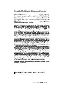
Fig. 11.3 An example hierarchical hidden Markov model. Only leaf nodes produce observations. Internal nodes can be viewed as generating sequences of observations.

11.3.2

Hierarchical Hidden Markov Models

Hidden Markov models (HMMs) are a widely-used probabilistic model for representing time-series data, such as speech [11]. Unlike an MDP, states are not perceivable, and instead the agent receives an observation o which can be viewed as being generated by a stochastic process P (o|s) as a function of the underlying state s. HMMs have been widely applied to many time-series problems, ranging from speech recognition [11], information extraction [8], and bioinformatics [12]. However, like MDPs, HMMs do not provide any direct way of representing higher-level structure that is often present in many practical problems. For example, an HMM can be used as a spatial representation of indoor environments [34], but typically such environments have higher order structures such as corridors or floors which are not made explicit in the underlying HMM model. As in the case with MDPs, in most practical problems, the parameters of the underlying HMM have to be learned from samples. The most popular method for learning an HMM model is the Baum-Welch procedure, which is itself a special case of the more general Expectation-Maximization (EM) statistical inference algorithm. Recently, an elegant hierarchical extension of HMMs was proposed [7]. The HHMM generalizes the standard hidden Markov model by allowing hidden states to represent stochastic processes themselves. An HHMM is visualized as a tree structure (see Figure 11.3) in which there are three types of states, production states (leaves of the tree) which emit observations, and internal states which are (unobservable)

SPATIOTEMPORAL ABSTRACTION OF MARKOV PROCESSES

291

hidden states that represent entire stochastic processes. Each production state is associated with an observation vector which maintains distribution functions for each observation defined for the model. Each internal state is associated with a horizontal transition matrix, and a vertical transition vector. The horizontal transition matrix of an internal state defines the transition probabilities among its children. The vertical transition vectors define the probability of an internal state to activate any of its children. Each internal state is also associated with a child called an end-state which returns control to its parent. The end-states (e1 to e4 in Figure 11.3) do not produce observations and cannot be activated through a vertical transition from their parent. Figure 11.3 shows a graphical representation of an example HHMM. The HHMM produces observations as follows: 1. If the current node is the root, then it chooses to activate one of its children according to the vertical transition vector from the root to its children. 2. If the child activated is a product state, it produces an observation according to an observation probability output vector. It then transitions to another state within the same level. If the state reached after the transition is the end-state, then control is returned to the parent of the end-state. 3. If the child is an abstract state then it chooses to activate one of its children. The abstract state waits until control is returned to it from its child end-state. Then it transitions to another state within the same level. If the resulting transition is to the end-state then control is returned to the parent of the abstract state. The basic inference algorithm for hierarchical HMMs is a modification of the “inside-outside” algorithm for stochastic context-free grammars, and runs in O(T 3 ), where T is the length of the observation sequence. Recently, Murphy developed a faster inference algorithm for hierarchical HMMs by mapping them onto a dynamic Bayes network [23]. 11.3.3

Factored Markov Processes

In many domains, states are composed of collections of objects, each of which can be modeled as a multinomial or real-valued variable. For example, in driving, the state of the car might include the position of the accelerator and brake, the radio, the wheel angle, and so on. Here, we assume the agent-environment interaction can be modeled as a factored semi-Markov decision process, in which the state space is spanned by the Cartesian product of random variables X = {X1 , X2 , ..., Xn }, where each Xi takes on values in some finite domain Dom(Xi ). Each action is either a primitive (single-step) action or a closed-loop policy over primitive actions. Dynamic Bayes networks (DBNs) [5] are a popular tool for modeling transitions across factored MDPs. Let Xit denote the state variable Xi at time t and Xit+1 the variable at time t+1. Also, let A denote the set of underlying primitive actions. Then, for any action a ∈ A, the Action Network is specified as a two-layer directed acyclic

292

HIERARCHICAL APPROACHES TO CONCURRENCY, MULTIAGENCY, & P. O.

graph whose nodes are {X1t , X2t , ..., Xnt , X1t+1 , X2t+1 , ..., Xnt+1 } and each node Xit+1 is associated with a conditional probability table (CPT) P (Xit+1 |φ(Xit+1 ), a) in which φ(Xit+1 ) denotes the parents of Xit+1 in the graph. Qn The transition probability P (X t+1 |X t , a) is then defined by: P (X t+1 |X t , a) = i P (Xit+1 |wi , a) where wi is a vector whose elements are the values of the Xjt ∈ φ(Xit+1 ). Figure 11.4 shows a popular toy problem called the Taxi Problem [6] in which a taxi inhabits a 7-by-7 grid world. This is an episodic problem in which the taxi (with maximum fuel capacity of 18 units) is placed at the beginning of each episode in a randomly selected location with a randomly selected amount of fuel (ranging from 8 to 15 units). A passenger arrives randomly in one of the four locations marked as R(ed), G(reen), B(lue), and Y(ellow) and will select a random destination from these four states. The taxi must go to the location of the passenger (the “source”), pick up the passenger, move to the destination location (the “destination”) and put down the passenger there. The episode ends when either the passenger is transported to the desired destination, or the taxi runs out of fuel. Treating each of taxi position, passenger location, destination and fuel level as state variables, we can represent this problem as a factored MDP with four state variables each taking on values as explained above. Figure 11.4 shows a factorial representation of taxi domain for Pickup and Fillup actions. While it is relatively straightforward to represent factored MDPs, it is not easy to solve them because in general the solution (i.e., the optimal value function) is not factored. While a detailed discussion of this issue is beyond the scope of this article, a popular strategy is to construct an approximate factored value function as a linear summation of basis functions (see [15]). The use of factored representations is useful not only in finding (approximate) solutions more quickly, but also in learning a factored transition model in less time. For the taxi task illustrated in Figure 11.4, one idea that we have investigated is to express the factored transition probabilities as a mixed memory factorial Markov model [33]. Here, each transition probability (edge in the graph) is represented a weighted mixture of distributions, where the weights can be learned by an expectation maximization algorithm. More precisely, the action model is represented as a weighted sum of crosstransition matrices: P (xit+1 |Xt , a) =

n X

ψai (j)τaij (xit+1 |xjt ),

(11.2)

j=1

where the parameters τaij (x0 |x) are n2 elementary × k transition matrices and Pk n parameters ψai (j) are positive numbers that satisfy j=1 ψai (j) = 1 for every action a ∈ A (here, 0 ≤ i, j ≤ n, where n is the number of state variables). The number of free parameters in this representation is O(|A|n2 k 2 ) as opposed to O(|A|k 2n ) in the non-compact case. The parameters ψai (j) measure the contribution of different state variables in the previous time step to each state variable in the current state. If the problem is completely factored, then ψ i (j) is the identity matrix whose ith component is independent of the rest. Based on the amount of factorization that exists

SPATIOTEMPORAL ABSTRACTION OF MARKOV PROCESSES

293

in an environment, different components of ψai (j) at one time step will influence the ith component at the next. The cross-transition matrices τaij (x0 |x) provide a compact way to parameterize these influences.

R

G

F

t

Fillup

Taxi position

Taxi position

passenger location

passenger location

Destination

Destination

Fuel

Y

t+1

Fuel

B

Fig. 11.4 The taxi domain is an instance of a factored Markov process, where actions such as fillup can be represented compactly using dynamic Bayes networks.

Figure 11.5 shows the learning of a factored MDP compared with a table-based MDP, averaged over 10 episodes of 50000 steps. Each point on the graph represents the RMS error between the learned model and the ground truth, averaged over all states and actions. The FMDP model error drops quickly in the early stages of the learning in both problems. Theoretically, the tabular maximum likelihood approach (which estimates each transition probability as the ratio of transitions between two states versus the number of transitions out of a state) will eventually learn the the exact model if every pair of states and action are visited infinitely often. However, the factored approach which uses a mixture weighted representation is able to generalize much more quickly to novel states and overall model learning happens much more quickly. 11.3.4

Structural Decomposition of Markov Processes

Other related techniques for decomposition of large MDPs have been explored, and some of these are illustrated in Figure 11.6. A simple decomposition strategy is to split a large MDP into sub-MDPs, which interact “weakly” [4, 25, 37]. An example of weak interaction is navigation, where the only interaction among sub-MDPs is the states that connect different rooms together. Another strategy is to decompose a large MDP using the set of available actions, such as in air campaign planning problem [21], or in conversational robotics [26]. An even more intriguing decomposition strategy is when sub-MDPs interact with each other through shared parameters. The transfer line optimization problem from manufacturing is a good example of such a parametric decomposition [44].

294

HIERARCHICAL APPROACHES TO CONCURRENCY, MULTIAGENCY, & P. O.

Taxi domain 0.16

Tabular Maximum-Likelihood FMDP

0.14

RMS Error

0.12 0.1 0.08 0.06 0.04 0.02 0 0

10000

20000

30000

40000

50000

Steps

Fig. 11.5

Comparing factored versus tabular model learning performance in the taxi domain.

$

Available Action Set

x $ Room 1

x x x x

Room 2 x x

x

x

x

MTS

x x Room 3

Room 4

x

x

Task 1 a)

Fig. 11.6

11.4

Task 2

Task n

b)

State and action-based decomposition of Markov processes.

CONCURRENCY, MULTIAGENCY, AND PARTIAL OBSERVABILITY

This section summarizes our recent research on exploiting spatiotemporal abstraction to produce improved solutions to three difficult problems in sequential decisionmaking: (1) learning plans involving concurrent action, (2) multiagent coordination, and (3) using memory to estimate hidden state. 11.4.1

Hierarchical Framework for Concurrent Action

We now describe a probabilistic model for learning concurrent plans over temporally extended actions [30, 31]. The notion of concurrent action is formalized in a general way, to capture both situations where a single agent can execute multiple parallel

CONCURRENCY, MULTIAGENCY, AND PARTIAL OBSERVABILITY

295

processes, as well as the multi-agent case where many agents act in parallel. The Concurrent Action Model (CAM) is defined as (S, A, T , R), where S is a set of states, A is a set of primary actions, T is a transition probability distribution S × wp(A) × S × N → [0, 1], where wp(A) is the power-set of the primary actions and N is the set of natural numbers, and R is the reward function mapping S →