1.2
PRELIMINARY RESULTS FROM THE ETL OPEN OCEAN AIR-SEA FLUX DATABASE C. W. Fairall *, J. E. Hare, and A. A. Grachev NOAA Environmental Technology Laboratory (ETL) Boulder, CO E. F. Bradley CSIRO Land and Water Canberra, Australia J. B. Edson Woods Hole Oceanographic Insitution Woods Hole, MA
1.
The transfer coefficients have a dependence on surface stability prescribed by MOS
INTRODUCTION
The COARE 2.5 algorithm (Fairall et al. 1996a) was developed for the Coupled Ocean Atmosphere Response Experiment (COARE) program (Webster and Lukas 1992) and has been evaluated against several sets of tropical data. It performs well, as do several other algorithms (Zeng et al. 1998). None of the new algorithms have been extensively tested against a large and latitudinally diverse data base. A joint CSIRO/ETL effort has been underway to use new data to evaluate the algorithm, continue improvements, and add better physics; this led to the recent issuance of a version 2.6 (Bradley et al. 2000). In this paper we evaluate the accuracy of version 2.6 against a database from 12 ETL flux cruises with about 5000 hr of usable direct flux measurements. 2.
, (3)
where > is the MOS stability parameter, the subscript n refers to neutral (> = 0) stability, z is the height of measurement of the mean quantity [X(z)], R an empirical function describing the stability dependence of the mean profile, 6 is von Karman’s constant, and zox parameter called the roughness length that characterizes the neutral transfer properties of the surface for the quantity, x. The MOS stability parameter is given by
BACKGROUND .
Bulk algorithms to estimate surface fluxes are widely used in numerical models and in applications (e.g., satellite retrievals) where highly detailed local information is not available. These are based upon Monin - Obukhov similarity (MOS) representations of the fluxes in terms of mean quantities (Smith et al. 1996) ,
(1)
where x can be the u, v wind components, the potential temperature, 2, the water vapor mixing ratio, q, or some atmospheric trace species mixing ratio. Here cx is the bulk transfer coefficient for the variable x (the d being used for wind speed) and Cx is the total transfer coefficient. )X is the sea-air difference in the mean value of x and S is the mean wind speed which is composed of a mean vector part (U and V components) and a gustiness part (Ug ) to account for subgridscale variability .
(2)
* Corresponding author address: C. W. Fairall, NOAA/ETL, 325 Broadway, Boulder, CO 80305-3328; e-mail:
[email protected]
(4)
The essence of the bulk model is contained in (1), (2), and (4) plus the representations (parameterizations) of the roughness lengths (or, equivalently the transfer coefficients) and the stability functions ( Rx ). While there are many algorithms available today and these will be considered in this work, for purposes of brevity we will restrict our comments in this paper to the TOGA COARE bulk algorithm (Fairall et al. 1996a). The velocity roughness length is specified via a Charnock plus a smooth flow limit
,
where
(5)
is the friction velocity. The scalar
roughness lengths are parameterized in terms of the roughness Reynolds number, . The stability functions are a blend of conventional well-determined overland functions near neutral stability with a form that obeys the theoretical scaling limit in highly convective conditions (Fairall et al. 1996a). In typical execution of a bulk algorithm, the atmospheric variables (U, V, T, q) at reference height z are provided through measurement or model output; the
Table 1. Summary of ETL air-sea flux and bulk meteorological data cruises used in the analysis. Cruise Name
Dates
Hours
Vessel
Latitude
Longitude
TIWE
11/21-12/13/91
460
Moana Wave
0
140 W
ASTEX
6/06-6/28/92
390
M. Baldrige
30 N
25 W
COARE-1
11/11/-12/03/92
589
Moana Wave
2S
156 E
COARE-2
12/17/-1/11/93
648
Moana Wave
2S
156 E
COARE-3
1/28/-2/16/93
385
Moana Wave
2S
156 E
SCOPE
9/17/-9/28/93
305
FLIP
33 N
118 W
FASTEX
12/23-1/24/97
730
Ron Brown
45 N
10-60 W
JASMINE
5/5-5/31/99
654
Ron Brown
8N
89 E
Nauru99
6/15-7/18/99
794
Ron Brown
0.5 S
167 E
KWAJEX
7/28-9/12/99
875
Ron Brown
8N
167.5 E
Moorings
9/14-10/21/99
746
Ron Brown
52 N
140 W
PACSF99
11/11-12/2/99
640
Ron Brown
±10 N
100 W
surface properties (surface current vector, water temperature) are also provided. Usually the water temperature at some depth, Tw(D), is given while the surface value is required by (1); the surface value for specific humidity is computed from the surface temperature and the vapor pressure of seawater (0.98 times the vapor pressure of pure water). If the true interface water temperature is not provided, then some method of estimating Ts from Tw must be used. In the COARE model this is accomplished through submodels that represent the millimeter-scale cool skin near the interface and the diurnal (solar) warm layer in the upper few meters of the ocean (Fairall et al. 1996b). Finally, in the COARE algorithm, the gustiness is represented as boundary-layer scale large eddies using the convective velocity scale ,
(6)
where $ is a parameter presently set to 1.25. 3.
IMPROVEMENTS IN COARE ALGORITHM
The published version (2.5b) of the COARE algorithm is in widespread use but the Flux Working Group has continued to pursue improvements in the various components of the model. A new version of the model (2.6a) has been made public; the changes are summarized in Bradley et al. (2000). Aside from various structural improvements, the neutral transfer coefficients have been ajdusted slightly. The Liu et al. (1979) scalar roughness relationship [ fx(Rr) ] has been replaced with a much simpler one that fits both the COARE and HEXMAX data bases and the Charnock parameter has been given a slight wind speed dependence for winds between 10
and 18 ms-1. These changes were intended to extend the algorithm’s region of applicability from a maximum wind speed of 10 ms-1 to 20 ms-1. Matlab and Fortran versions of both COARE 2.5b and 2.6a have been made publically available at the ftp site at ETL: ftp://ftp.etl.noaa.gov/et7/users/cfairall/bulkalg/. Included is a description of the codes and a test data set file. The programs are set up to read the test file and output the results; output files and graphs of results are also provided. 4.
ADDITIONS TO THE FLUX DATABASE
Version 2.6 was based on fits to ETL flux data from six cruises in the early 1990's plus published results on fluxes at high wind speeds (DeCosmo et al. 1998; Yelland and Taylor 1996). Six new cruises obtained with the ETL seagoing flux system (Fairall et al. 1997) recently became available and were combined with the original six cruises (see Table 1). This larger database has more highlatitude measurements and includes about 800 hrs of data at wind speed greater than 10 ms-1. Because the initial ETL database of six cruises had only 67 hrs of data at wind speed greater than 10 ms-1, this new data allows us to test the in the wind speed range of 10 - 20 ms-1. 5. FLUX AND TRANSFER COEFFICIENT EVALUATION The first step in evaluating the performance of the flux algorithm is to select a subset of the data that pass a set of criteria to reject invalid points. Such criteria include experimental aspects (such as the relative wind must fall within a certain range to eliminate obvious contamination by the ship’s structure), instrument performance indicators, ship motion-correction errors associated with ship maneuvers, and requirements that certain variables
COARE 2.6A. 14th Symposium on Boundary Layer and Turbulence, AMS. 7 - 11 August 2000, Aspen CO, 294-296. DeCosmo, J., K. B. Katsaros, S. D. Smith, R. J. Anderson, W. A. Oost, K. Bumke, and H. Chadwick, 1996: Air-sea exchange of water vapor and sensible heat: The Humidity Exchange Over the Sea (HEXOS) results. J. Geophys. Res., 101, 12001-12016. Fairall, C. W., E. F. Bradley, D.P. Rogers, J. B. Edson, and G. S Young, 1996a: Bulk parameterization of air-sea fluxes in TOGA COARE. J. Geophys. Res., 101, 3747-3767. Fairall, C. W., E. F. Bradley, J. S. Godfrey, G.A. Wick, J. B. Edson, and G. S. Young, 1996b: Cool skin and warm layer effects on the sea surface temperature. J. Geophys. Res., 101, 1295-1308. Fairall, C.W., A.B. White, J.B. Edson, and J.E. Hare, 1997: Integrated shipboard measurements of the marine boundary layer. J. Atmos. Oceanic Tech., 14, 338-359. Liu, W. T., K. B. Katsaros, and J. A. Businger, 1979: Bulk parameterization of the air-sea exchange of heat and water vapor including the molecular constraints at the interface. J. Atmos. Sci., 36, 2052-2062. Smith, S. D., C. W. Fairall, G. L. Geernaert, and L. Hasse, 1996: Air-sea fluxes: 25 years of progress. Bound.-Layer Meteorol., 78, 247-290. Yelland, M. and P. K. Taylor, 1996: Wind stress measurements from the open ocean. J. Phys. Oceanogr., 26, 541-558. Webster, P. J., and R. Lukas, 1992: The Coupled Ocean Atmosphere Response Experiment. Bull. Am. Met. Soc., 73, 1377-1416. Zeng, X., M. Zhao, and R. E. Dickinson, 1998: Comparison of bulk aerodynamic algorithms for the computation of sea surface fluxes using the TOGA COARE and TAO data. J. Clim., 11, 2628-2644.
300
250
200 Hl (W/m2)
(e.g., variances) fall within physically reasonable limits. The criteria are arbitrary but the results are only weakly affected by modest criteria changes. Both direct covariance and inertial-dissipation (ID) flux estimates are used in our analysis. The next step is to compare the values of fluxes obtained from the bulk algorithm with the measurements in some rational fashion. Usually we are interested in the average performance of the bulk algorithm plus some information on its statistical scatter about the observations. One can compute mean and standard deviations of differences, linear regressions, etc. In this paper we will show mean comparisons averaged in bins of 10-m neutral wind speed. Fig.1 shows a comparison of the mean latent heat flux computed in wind speed bins from 0 to 22 ms-1. The width of the bins is increased slightly at higher wind speeds where the density of data decreases. The turbulence values are the average of covariance and ID values; the bulk values (x’s) are COARE 2.6. We have used both medians and means to indicate skewed distributions or effects of outliers. Fig. 2 shows these same values plotted on a linear scale as flux vs flux. Fig. 3 shows a similar x - y plot for stress, except we have used only medians and have averaged the covariance and ID values separately; the display is log-log because of the much greater dynamic range of stress. Figs. 2 and 3 suggest very close agreement between the model and the data, but a more critical test comes when we evaluate the transfer coefficients (Eq. 1). Because of the noisy nature of flux data and the difficulties of making very accurate bulk meteorological measurements, the experimental evaluation of transfer coefficients is problematical. Using (1) we can compute a transfer coefficient for each observation and average in wind speed bins (method 1). Or, we can average the fluxes and bulk variables in wind speed bins, compute ‘effective’ transfer coefficients that deliver the correct average flux (method 2). Another approach is to compute an average transfer coefficient that is the mean bulk coefficient times the ratio of the mean measured flux to the mean computed bulk flux (method 3). We have experimented with these (and other) approaches; at the moment we weakly favor method 3. Our results are shown for moisture flux (Fig. 4) and stress (Fig. 5). The data for both variables show a tendency for slightly lower transfer coefficients for wind speeds below 8 ms-1 and greater transfer coefficients for greater wind speeds. Surprisingly, the moisture roughness length parameterization is in good agreement with the data; the difference in transfer coefficient for moisture is caused by the velocity contribution (i.e., the cd1/2 part of Eq. 1).
150
100
50
ACKNOWLEDGMENTS
This work is directly supported by the Office of Naval Research, the NSF Office of Climate Dynamics, The Department of Energy ARM program, and the NOAA Office of Global Programs. REFERENCES Bradley, E. F., C. W. Fairall, J. E. Hare, and A. A. Grachev, 2000: An old and improved bulk algorithm for air-sea fluxes:
0 0
5
10 u10n (m/s)
15
20
Fig. 1. Mean (line) and median (no line) fluxes computed in wind speed bins for 4272 selected hours of latent heat flux data. The x’s are COARE 2.6 values; the circles are the average of covariance and ID values.
0
250
10
200
150
Taucx, Tauib
Turb Hl (W/m2)
-1
10
100
-2
10
50 -3
10
0 0
100 150 200 250 2 Bulk Hl (W/m ) Fig. 2. The same data points from Fig. 1 but plotted as bulk latent heat flux values versus turbulent values. The x’s are the means; the circles are medians.
-2
-1
10
0
10
10
Taub
Fig. 3. As in Fig. 2 but for turbulent stress. The circles are the covariance values; the diamonds are the inertial-dissipation values. Negative covariances at very low winds are not shown.
-3
-3
1.4
-3
10
50
x 10
x 10
2.4 1.35
2.2 1.3
2 1.8 Cd10n
CE10n
1.25 1.2
1.6
1.15
1.4
1.1
1.2
1.05
1
1 0
5
10 U10n (m/s)
15
20
Fig.. 4. Median moisture 10-m neutral transfer coefficient as a function of 10-m neutral wind. The diamonds are computed with method 1 (see text); the circles with method 3. Errors bars indicate the statistical uncertainty (one sigma) of the mean estimate based on the distribution within the wind speed bin. The heavy solid line is COARE 2.6
0.8 0
5
10 U10n (m/s)
15
20
Fig. 5 Median 10-m neutral velocity transfer coefficient as a function of 10-m neutral wind. The circles are computed with 3. Errors bars indicate the statistical uncertainty (one sigma) of the mean estimate based on the distribution within the wind speed bin. The heavy solid line is COARE 2.6