Cost-Effective Condition-Based Maintenance Using Markov Decision Processes Suprasad V. Amari, Ph.D., Relex Software Corporation Leland McLaughlin, Relex Software Corporation Hoang Pham, Ph.D., Rutgers University Key Words: Cost-Effective Solution, Condition-Based Maintenance (CBM), Markov Decision Process (MDP) SUMMARY & CONCLUSIONS Investigations conducted in several industries indicate that there is no direct relationship between equipment failure and equipment age in the majority of cases. Most failures are caused by events or conditions that occur during component operation and manufacturing processes. Therefore, optimal maintenance decisions should be based on the actual deterioration conditions of the components. Condition-Based Maintenance (CBM) is a methodology that strives to identify incipient faults before they become critical to enable more accurate planning of preventive actions. For the ultimate success of CBM methodology, we must have sound methods for modeling deterioration (the propagation of faulty conditions), the conditions and their effects, and the optimal selection and scheduling of inspections and preventive maintenance actions (the right action at the right time). In this paper, we present a generalized CBM model that can be applied to a wide range of applications. The CBM model includes a stochastic deterioration process, a set of maintenance actions and their effects, and a scheduled inspection policy that identifies the condition of deterioration. Using Markov Decision Processes (MDP), we provide an optimal cost-effective maintenance decision based on the condition revealed at the time of inspection. In addition, we present a procedure for finding optimal inspection schedules. 1. INTRODUCTION System performance, productivity, and associated gain can be improved by using efficient maintenance policies. Knowledge of equipment failure mechanisms, causes, symptoms, detection and diagnosis procedures, and corrective and preventive mechanisms all play vital roles in the proper implementation of a maintenance program. However, few companies utilize this knowledge in an effective and systematic way. One reason for this might be the insufficient maturity level in the methods available for analyzing maintenance-related data and providing cost-effective maintenance decisions [1]. In this paper, we present a systematic procedure to perform cost-effective conditionbased maintenance (CBM) decisions.
1.1 Acronyms & Abbreviations CBM CM MDP MM MR NA PDM PM TBM
Condition-Based Maintenance Corrective Maintenance Markov Decision Process Minor Maintenance Minimal Repair No Action Predictive Maintenance Preventive Maintenance Time-Based Maintenance
1.2 A Brief Overview of Traditional Maintenance Models Traditional maintenance policies include corrective maintenance (CM) and preventive maintenance (PM). With CM policy, maintenance is performed after a breakdown or the occurrence of an obvious fault. With PM policy, maintenance is performed to prevent equipment breakdown. PM policy uses time-based maintenance (TBM) schedules to determine equipment replacement. For example, equipment might be replaced at the age of 2 years (age replacement) or in the first week of every quarter (constant time replacement). Some variations to TBM include group maintenance and virtual age-based maintenance. The main assumption in TBM models is that the chance of a component failure depends entirely on the age of the component. This means that two components of same type and same age have the same failure rate, regardless of the events that have occurred during their operation or the manufacturing process. These models are based on the concept of the bathtub curve, where hazard rate increases in a predetermined way. However, investigations conducted on United Airlines aircraft components indicate that only 3% to 4% of equipment failures can be explained using traditional bathtub curve type hazard functions [1]. The U.S. Navy conducted similar investigations and confirmed these findings. Additionally, several independent studies across various industries indicate that only about 15% to 20% of equipment failures are age-related. The other 80% to 85% of equipment failures are based totally on the effects of random events that happen in the system. This means that TBM is inappropriate in most cases.
1-4244-0008-2/06/$20.00 (C) 2006 IEEE
1.3 Reasons for Equipment Failures A proper understanding and modeling of age-independent failure behavior is important. If failure is solely dependent on the age of the component, then all components of the same type should fail at the same time. However, this is not true because varying levels of latent defects and impurities can exist. This leads to different rates or patterns of defect propagation. Moreover, variations in raw material, loads, operator skills, maintenance activities, and other events such as floods and earthquakes can all influence the failure mechanisms. The presence of defective components in the system may also cause damage to other components. For example, failure of a bearing shaft can depend on the conditions of the bearing casing, the lubrication process, and vibrations of the equipment structure. Therefore, the failure propagation is a complex stochastic process not only depends on age but also depends on several other factors and events. 1.4 Failure Rate vs. Maintenance Actions When the effects of age on the failure are less influential than other factors, there may not be any correlation between failure and age. When the failure rate is expressed as a function of time, it may not follow the bathtub curve. In addition, even though the failures rates of individual components are strictly increasing, the overall failure rate of the population can have a decreasing trend [1]. However, this does not mean that the hazard rate is meaningless or that preventive actions are unnecessary. There may be some other factor, such as temperature rise, vibration level, or corrosion deposit that accurately explains the failure rate. In most cases, the failure rate depends on a combined index of various factors such as corrosion and deformation. Therefore, if we fit the failure distribution with respect to these other factors that cause the failure, we may find an increasing failure rate function. This is an example where we employ preventive actions when failure rate with respect to time is nonincreasing, but it is increasing with some other measurable factor such as wear. An example of wear-based maintenance is the replacement of a car tire. 1.5 Deterministic vs. Stochastic Deterioration In most reliability textbooks, the reason for an increasing failure rate is explained as the effects of wear and tear (deterioration). Therefore, the failure distributions that represent increasing failure rates, such as Weibull and Gamma distributions, are recommended. However, the well-defined failure rate as a function of time is an indication of a deterministic wear propagation (deterioration) process, which is a major limitation of time-based models. The second limitation is the inherent assumption that age can be observed but not deterioration. However, in the majority of cases, we can measure deterioration. For example, deterioration can be a reduction in shaft diameter or impurities in oil analysis. Therefore, whenever possible, it is better to perform the maintenance based on the level of deterioration, which is the basis for CBM models. For a detailed discussion, refer to [1].
2. CONDITION-BASED MAINTENANCE CBM, which is an effective form of predictive maintenance (PDM), is based on detecting causes or symptoms of a future failure early so that this failure can be handled most cost effectively before its occurrence. CBM actions are performed based on actual equipment condition, rather than on time or usage interval. Vibration measurement on rotating equipment is probably the best known of current predictive applications, but other categories of industrial equipment also benefit from a CBM approach. A spectrum of traditional PDM that include equipment type and category, failure mode and cause, and the detection method is provided in [1]. With traditional PDM, the condition of the system is predicted based on the trend of measures of physical parameters against established engineering limits for the purpose of detecting, analyzing, and correcting problems before failure occurs. The physical parameters are measured periodically (weekly, biweekly, monthly, etc.). If the measurement exceeds the established limit, it must be analyzed further. For example, a vibration signature can be taken on rotating equipment. A trained analyst can review the signature for the presence of problems such as misalignment, imbalance, and resonance. Correction of the root problem is the key to most predictive efforts. The traditional PDM cycle is graphically shown in Figure 1. Periodic Monitoring No
Repair Equipment
Measurement Exceeds Engineering Limit?
Yes
Analyse Problem
Figure 1: Traditional PDM Cycle In the traditional PDM approaches, the decision is either to correct the problem completely or to take no action. However, CBM decisions can include a wide range of actions, such as: 1. Adjustments to the equipment. An adjustment can be a simple fine-tuning of a cam on a limit switch or involve the tuning of a boiler combustion control system to maximize fuel efficiency. 2. Replacement of damaged or warn components. 3. Replacement of disposable components such as air, oil, or fuel filters. 4. Performance of an overhaul that aims to restore the equipment to as-good-as-new condition. Some advantages of CBM are: 1. Reduction in the total maintenance program cost. 2. Avoidance of very disruptive equipment outages. 3. Reduction of costly PM activities when condition assessment shows no need of the scheduled maintenance.
CBM not only reduces the amount of maintenance performed but also avoids maintenance-induced failures. A review on CBM-related technologies and the strengths and weaknesses of various maintenance models is presented in [1]. 2.1 CBM Requirements The effective implementation of CBM involves the following tasks. 1. Identify failure mechanisms, causes, and detection and prevention methods. This involves the engineering aspects of the system under study. A review of the existing standards that provide such knowledge is presented in [4]. 2. Identify the deterioration model associated with the system. The model can be built using the knowledge of failure mechanisms as well as the existing data related to failures. Hidden Markov models, data mining techniques, and statistical techniques can be used for this purpose. 3. Determine the costs and effects associated with the various kinds of failures and maintenance actions. 4. Develop an optimal CBM policy that involves optimal inspection schedules for condition monitoring and the optimal maintenance decisions. This is the main contribution of this paper. An overview of current practices for CBM decisions is provided in reference [3]. 3. RELATED WORK 3.1 Deterioration Models To incorporate the stochastic nature of the deterioration process, researchers introduced multi-stage deterioration models using Markov chains. In these models, the system can have several stages of unidirectional deterioration. The first stage is the good stage, and the last stage is the failed stage. In addition to deterioration failures, the system can also fail randomly (Poisson failure) from any stage where the failure rate varies with the system deterioration stage. Multi-stage deterioration models are further extended to incorporate the CBM concepts of periodic inspections and deterioration stagebased maintenance actions such as no action (NA), minimal maintenance (MM), and preventive maintenance (PM), which is also called major maintenance. In addition to this, a minimal repair (MR) is performed upon a Poisson failure, and a corrective maintenance (CM) is performed upon a deterioration failure. The description of a commonly used CBM model follows: 1. The system is subjected to k stages of deterioration. 2. The system is subjected to periodic inspections. 3. Following an inspection, based on the current deterioration value of i, one of these steps is taken: a. 1 ≤ i ≤ n1 : NA is performed; the system is returned to its operation. b. n1 < i < n2 : MM is performed; the system is returned to its previous deterioration stage. c. n2 ≤ i ≤ k : PM is performed; system reaches the perfectly good stage.
Following the completion of k stages of deterioration, which is failure, a CM is performed so that the system is restored to an as-good-as-new condition. 5. Upon a Poisson failure, a MR is performed so that the system is returned to its operation with no change in its deterioration level. Several extensions and special cases of this model are studied in the literature. They include state independent Poisson failures ( λ = λi ), general distributions for failures and repairs, and deterministic (fixed) time inspection intervals. 4.
3.2 Limitations of Existing CBM Models 1.
Inspection Distribution: The major limitation with existing CBM models is that the exponentially distributed inspection intervals do not help engineers to determine when to perform inspections. 2. Inspection Schedule: The existing CBM models assume that inspections intervals are independent of the system deterioration condition, which is an inefficient schedule. This leads to performing inspections unnecessarily when the system is functioning properly. Additionally, it leads to not performing inspections when there is a need. 3. Deterioration Model: The existing CBM models are limited to unidirectional, single-step deterioration that neither models the combined effects of various deterioration mechanisms nor the effects of random events such as floods and earthquakes. 4. CBM Decisions: In existing models, only a few kinds of CBM decisions are considered: NA, MM, and PM. In reality, there can be several types of maintenance decisions such as refill the lubricant, replace the screws, align the bearing, and replace the bearing. 5. Effects of Maintenance: All existing CBM models support only the maintenance actions that reduce the current deterioration level. However, in some cases, the CBM actions may reduce the rate of deterioration instead of actual deterioration. For example, the wear propagation of a cutting tool can be reduced by changing the cutting depth, cutting speed, or the lubrication flow rate. 6. Optimization Procedure: Another major disadvantage of existing CBM models stems from their procedures for finding the optimal decisions. The existing models first find a closed-form cost function and then compute the cost for all possible combinations of parameters to find the minimal cost. This approach is feasible only for simple deterioration processes and a limited number of decision variables. Therefore, we need better models and algorithms for handling all kinds of complex situations that arise in practical CBM decision-making. For a detailed discussion, refer to [1]. 4. CBM MODEL 4.1 Deterioration 1.
The system deterioration is a function of a set of deterioration parameters. Example: deformation level,
corrosion level, diameter of shaft, temperature, depth of cut, and lubrication condition. 2. Each parameter may again be subjected to stochastic deterioration, which can depend on other deterioration parameters (as well as the CBM actions performed). 3. For each parameter, the deterioration level can be described in discrete levels or categories. 4. Some deterioration stages themselves can be considered as failures. The failure of the system can be identified immediately or only through inspection. Therefore, all of these scenarios can be modeled using acyclic Markov chains. 4.2 Inspections 1. 2. 3. 4.
The system is subjected to scheduled inspections. Inspections reveal the system condition (state) perfectly. Cost of inspection may vary based on system condition. The schedule for the next inspection depends on the current system condition.
4.3 Actions Based on CBM Decisions 1. 2.
3. 4. 5.
6.
A CBM decision is a combination of two decisions: maintenance action and the next inspection schedule. CBM decisions can be categorized into two types: (a) decisions based on inspection results, and (b) pre-fixed decisions triggered by self-announcing system conditions; e.g., CM after a deterioration failure. Based on the condition revealed by the inspection, a specific CBM action is performed. One of the possible maintenance actions can be “no action” or “do nothing.” A system-level action can be a unique combination of several lower-level actions. For example, the action “Type-A maintenance” can be a combination of “rotate tires,” “change oil filter,” and “fill windshield fluid.” The results of a maintenance action need not be deterministic (cannot be predicted precisely) and may depend on various factors that cannot be controlled. Therefore, there can be a set of possible system states that can be reached after a maintenance action.
4.4 Cost Factors 1. 2. 3. 4.
A cost is associated with each inspection. The cost may vary with the system condition. A cost is associated with each maintenance action. The cost can also include system downtime cost. There is a cost per unit time for each undetected failure. A cost is associated with each failure.
a decision strategy to optimize a particular criterion such as minimizing the total cost [5]. MDP not only provides the consequences of a policy, but it also guarantees that no better policy exists [5]. A tutorial on MDP is provided in [6]. 5.2 Existing Difficulties in Solving CBM The CBM model considered here does not fall into any standard MDP formulation. One reason is that the maintenance actions are discrete and the inspection intervals are continuous. Another difficulty arises from the complex nature of the cost structure and decision epochs. To make use of the available well proven algorithms, we convert the CBM problem as a Semi-MDP formulation. The solution is provided using the well known policy iteration algorithm. 5.3 Standard Semi-MDP Solution The MDP has a set of states ( S ). For each state s ∈ S , a set of actions As are available. The action a performed in state s: • Brings the system to state s ' with probability P (s, s ', a ) . •
Produces an expected immediate cost r (s, a ).
•
Takes an expected transition time y(s, a ). A policy π is a mapping from s ∈ S to a ∈ As , where
π(s ) = a. The objective is find the optimal policy π * that minimizes average cost ( ρ ) in a long run. Let Rπ (s ) be the average cost associated with policy π , given that the system is in state s ∈ S . The policy iteration algorithm follows: 1. Select an arbitrary policy: π = π0 . 2. Value determination: Arbitrarily select a state s0 ∈ S and set Rπ (s 0 ) = 0. Solve the following equations for unknowns: ρπ and Rπ (s ), s ∈ S ; s ≠ s0 .
Rπ (s ) = r (s, π(s )) − ρπ ⋅ y(s, π(s )) +
∑ P(s, s ', π(s)) ⋅ Rπ (s '),
s ∈S
(1)
s ' ∈S
Policy improvement: For each s ∈ S , determine the alternative action a ' ∈ As that yields: r (s, a ') − ρπ ⋅ y(s, a ') , s ∈ S arg min (2) + ∑ P (s, s ', a ')Rπ (s ') a' s '∈S The resulting optimum actions for states s ∈ S constitute the new policy π ' . If π and π ' are identical, π is optimum. Otherwise, set π = π ' : go to step 2. To find the cost-effective CBM policy, the inputs for the MDP algorithm should be computed from the CBM model. 3.
5. MARKOV DECISION PROCESS
6. COST-EFFECTIVE CBM SOLUTION
5.1 MDP Basics
6.1 Inputs
An MDP is similar to a Markov process, except that the decision maker must make decisions at various time epochs. The goal of an MDP is to provide an optimal policy, which is
1.
MC: Markov Chain for the deterioration model. S : state space of MC.
S f : set of failed states; S f ⊂ S . .
a.
Sr : set of states where the system condition is revealed without inspections; Sr ⊂ S . S p : set of states where the maintenance actions are predetermined; S p ⊂ S .
b.
If the system state is revealed prior to the scheduled inspection: go to step 2. Else, perform the scheduled inspection: go to step 1. 7. EXAMPLE
2.
Maintenance Actions M s : set of alternative maintenance actions in state s. If s ∈ S p , size(Ms ) = 1.
The proposed method is demonstrated through a simple hypothetical example of locomotive diesel engine. Detailed analyses of complex problems and associated MATLAB code are provided in a separate document [1], which can be obtained from the authors.
3.
Cost Structure cM (m ) : cost of maintenance action m ∈ M .
7.1 Problem Description
λij : transition rate from state i to state j.
cF (s ) : one time cost of each failure, where s ∈ S f . cI (s ) : cost of inspection in state s ∈ S ; s ∉ Se . cS (s ) : cost per unit time stay in state s ∈ S f ; s ∉ Se . 4.
qij (m ) : probability that maintenance action m ∈ M performed in state i brings the system to state j.
6.2 Algorithm 1.
2.
For each state s, select N values for the next inspection interval that are equally distributed over a possible range [1]. Let Ts be the set of possible values in state s. Solve the MC for pij (t ) and τij (t ) , where:
pij (t ) : Pr{state j at time t | initial state is i} τij (t ) : E{time spent in state j in (0, t) | initial state is i} 4.
Each CBM action a in state s is a combination of maintenance action m ∈ M s and the next inspection time t ∈ Ts . Hence, a = (m, t ). Let As be the all possible
The health condition (deterioration level) of the engine is classified into six stages, i.e., s ∈ S = {1, …, 6} . The first stage ( s = 1 ) is the perfect condition stage, and the last stage ( s = 6 ) is a failed stage. The failure of the engine can be identified without inspections. Upon a failure, the system is restored to perfect stage (s=1) through a CM. Inspections that include emission and vibration analysis can be performed to know the system deterioration condition perfectly at any time. Based on the system deterioration, one of the following maintenance actions can be performed: • NA: no change in system deterioration. • MM: restores to its pervious condition. • PM: restores to the perfect condition. The objective is to find the most cost-effective CBM policy,which provides the optimal maintenance actions and inspection intervals. The deterioration model is shown in Figure 2. 1 NA
CBM actions in state s: size(As ) = size(M s ).size(Ts ). 5.
For s, s ' ∈ S ; a = (m, t ) ∈ Ai ; compute P (s, s ', a ).
P (s, s ', a ) =
∑ qsk (m).τks ' (t )
(3)
For s ∈ S ; a = (m, t ) ∈ Ai ; compute y(s, a ).
y(s, a ) =
∑ ∑ qsk (m).τks ' (t )
(4)
s ' ∈S ;s ' ∉ Sr k ∈S
7.
For s ∈ S ; a = (m, t ) ∈ Ai ; compute r (s, a ).
r (s, a ) = cM (s, m ) +
∑ P(s, s ', a ) ⋅ cF (s ')
s ' ∈S f
λ 4
λ 5
The mean time between two successive deterioration stages is 1000 hours ( λ = 0.001 per hour). Further, 1. All failures are self-announcing. Hence: S f = Se = {6}. 2.
Cost of failure: s ∈ S f , cF (s ) = $5000.
3.
Cost of inspection: s ∉ Se,cI (s ) = $100.
qsk (m ) ⋅ τks ' (t ) ⋅ cS (s ')
4.
Cost of NA: cM (NA) = 0.
5.
Cost of MM: cM (MM ) = $1, 000.
∑
P (s, s ', a ) ⋅ cI (s ')
6.
Cost of PM: cM (PM ) = $5, 000.
7.
Cost of CM: cM (CM ) = $7, 500.
8.
Cost of undetected failures: s ∈ S , cS (s ) = 0.
(5)
s ' ∈S ;s ' ∉ Sr
Using P (s, s ', a ), y(s, a ), and r (s, a ) , compute optimal policy using policy iteration algorithm.
6 CM
7.2 Inputs
∑
+
the
6.3 CBM Implementation as an MDP Policy 1. 2.
λ 3
s ' ∈S f ;s ' ∉ Sr
+
8.
λ 2
Figure 2: Deterioration Model
k ∈S
6.
λ
Find the current system condition (state). Based on the current state of the system, perform the maintenance action and schedule the next inspection as per the optimal policy.
7.3 Problem Formulation There are four types of maintenance actions: NA, MM , PM , and CM . The actions in s ∈ S p = {1, 5} are pre-determined.
M 1 = {NA}, M 6 = {CM }
(6)
The maintenance actions for s ∈ {2, 3, 4, 5} have to be determined. M 2 = M 3 = M 4 = M 5 = {NA, MM , MP } (7) If NA is performed, there is no change in the deterioration. 1 for i = j (8) qij (NA) = 0 for i ≠ j If MM is performed, one stage of deterioration is reduced. 1 for i = j + 1 (9) qij (MM ) = 0 for i ≠ j + 1 If PM or CM is performed, the system reaches the perfect stage. 1 for j = 1 qij (PM ) = qij (CM ) == (10) 0 for j ≠ 1 Further, inspection intervals must be determined for all states. 7.4 Optimal Solution The minimum and maximum possible values considered for the next inspection interval are 100 hours and 5000 hours. The range is divided equally to find the 20 possible values for the inspection interval. The initial policy is: π(s ) → (NA,100) for s ∈ {1, 2, 3, 4, 5} and π(6) → (CM ,100) The solution is stabilized within three policy iterations. The optimal policy is shown in Table 1. The corresponding average cost is ρ = $2.0002 per hour. State Maintenance Inspection Action Interval 1 NA 2163 2 MM 2163 3 MM 1390 4 MM 616 5 PM 2163 6 CM 2163 Table 1: Optimal CBM Policy 8. CONCLUSIONS The paper discusses the need for CBM methodologies and explains the limitations of time-based maintenance models as well as existing CBM models. A generalized CBM model that is applicable for a wide range of systems is presented. Using MDP, a generic procedure to obtain optimal inspection schedules as well as optimal maintenance decisions, is presented. The approach given in this paper offers reliability and maintenance engineers a practical and systematic procedure to perform CBM. REFERENCES 1.
S.V. Amari, A detailed version of the paper.
2. 3. 4. 5. 6.
F.S. Nowlan, H.F. Heap, “Reliability-centered maintenance”, U.S. Department of Commerce, 1978. A.K.S. Jardine, “Optimizing condition based maintenance decisions”, Proc. RAMS 2002, pp. 90-97. M. Bengtsson, “Condition based maintenance system technology - where is development heading?”, Proc. Euromaintenance, May 2004. M.L. Puterman, Markov Decision Processes, Wiley, 1994. http://www.autonlab.org/tutorials/mdp09.pdf (9-9-2005) BIOGRAPHIES
Suprasad V. Amari, PhD Relex Software Corporation 540 Pellis Road Greensburg, PA 15601 USA email:
[email protected] Suprasad Amari is a Senior Reliability Engineer at Relex Software Corporation. Dr. Amari received both his MS and PhD in Reliability Engineering from the Indian Institute of Technology, Kharagpur. He is an editorial board member of the International Journal of Reliability, Quality and Safety Engineering. He is a senior member of ASQ and IEEE, and member of IIE, SRE, SSS, and SOLE. Leland McLaughlin Relex Software Corporation 540 Pellis Road Greensburg, PA 15601 USA email:
[email protected] Leland McLaughlin has an extensive and diversified background in technical sales, engineering project management, and new market penetration. As Director of Global Sales and Marketing for Relex Software Corporation, he is responsible for coordinating and supervising Relex's international sales force. Hoang Pham, PhD Department of Industrial Engineering, Rutgers University, 96 Frelinghuysen Road Piscataway, NJ 08854 USA email:
[email protected] Dr. Hoang Pham is Professor at Rutgers University, Piscataway, NJ. He is the author of Software Reliability and the editor of the Handbook of Reliability Engineering among many others. He is editor-in-chief of the International Journal of Reliability, Quality and Safety Engineering. He is an editorial board member of several journals and has been conference chair and program chair of over 25 international conferences and workshops. He is a fellow of the IEEE.