14-1: Blow Simulation Test to Measure Coefficient of Friction between

Blow Simulation Test to Measure Coefficient of Friction between (Micro)Duct and Cable 1

W. Griffioen1, S. Zandberg2, P. M. Versteeg1, M. Keijzer3

Draka Comteq Telecom B.V., Zuidelijk Halfrond 11, 2801 DD Gouda, The Netherlands 2 Draka Comteq Telecom B.V., IJzerweg 2, 9936 BM Farmsum, The Netherlands 3 Vecom Metal Treatment B.V., Mozartlaan 3, 3144 NA Maassluis, The Netherlands +31-182-592490 · [email protected]

Abstract

2. Existing Test Methods

There is a need for a quick test to evaluate the blowing performance of a cable in a (micro)duct. An important parameter for this is the coefficient of friction (COF) between cable and (micro)duct. A summary is given of existing techniques to measure this parameter. It is concluded that none of these techniques offers sufficient reliable values to guarantee good blowing performance. In this paper an alternative technique, a blow simulation test, is described. Here a cable moves back and forth in a (micro)duct with airflow, simulating a “window” in a real field installation. The measured forces supply information on both friction and air drag force. Measurements show excellent correlation with blowing reference tests.

A summary is given of existing test methods to measure the COF between a cable and a (micro)duct.

2.1 Wheel Tests

Zwick or Instron

Keywords: Optical cable; microduct cable; duct; microduct; coefficient of friction; jetting; blowing; lubricant; lubricator.

R

1. Introduction For (micro)duct cabling a blowing test is needed to guarantee good blowing performance. Measurements of the coefficient of friction (COF) between (micro)duct and cable (or fibre unit) could serve as a quick alternative for blowing tests. Such tests would require less material and there would be no need to have a test trajectory. The blowing length in practical situations is than calculated from theory [1,2,3] (software exists which is based on this theory [4]), taking into account cable, (micro)duct and equipment properties and the typical undulations and bends in the trajectory. Many different techniques to measure the COF are used: wheel tests (different variants), sloped (micro)duct and cable tests and the bullet test from British Telecom [5].

M

In this paper the shortcomings of these techniques are listed. It appears that the correlation with blowing reference tests is poor. These matters are currently discussed in IEC 86A WG3, concerning the draft specification for microduct cabling [6]. Probably the only reliable tests until now turn out to be blowing reference tests themselves. For blown fibres (not cables) it is possible to perform such tests with the microduct on drum [7].

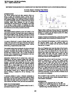
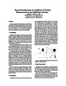
Figure 1. Sketch of a wheel test. A cable sample with attached weight is pulled through a (micro)duct sample around a wheel and the pulling force is measured. Several variants are used with different weights, diameters and angles over which the (micro)duct is pulled over the wheel. Sometimes also a pulley is used to direct the cable in line with the pulling/force-measuring device. One variant for use with microducts is given here as an example.

In this paper a new technique, a blow simulation test, is presented to measure the COF between (micro)duct and cable, based on but differing from the test of [8]. The cable is moved back and forth in a 17.1 m long (micro)duct while air is forced through. At the same time the force to move the cable is measured. The cablemoving equipment and force-measuring device are placed in a pressure chamber. The flow is such that real blowing conditions are simulated, e.g. the input and output pressures are the same as for a window of the same length in a blowing reference test. In this test the magnitudes of air-propelling force and COF can be acquired separately, showing e.g. the effect of textured cable surfaces. Tests so far have shown excellent correlation with blowing reference tests, also in cases where the wheel test failed.

International Wire & Cable Symposium

A wheel with radius R of 52 cm is placed before a pulling/forcemeasuring device, e.g. an Instron or Zwick, see Figure 1. The microduct sample is wound firmly around the wheel over 360º. The free angle φ for both microduct ends is about 10º (minimises effect of bending a cable with stiffness from straight to curved). A weight of which the mass M is about the mass of a length of 2 m

413

Proceedings of the 54th IWCS/Focus

extra friction due to spring action of the cable ends. The cable samples must be started by hand for the best result.

of the cable sample is attached to the cable. The force F to pull the cable through the duct (speed 1.0 or 1.8 m/min) after 20 cm of pulling is measured. A new clean, grease free cable sample has to be used to test every other duct sample. Sometimes a dummy cable, with the same weight but a lower stiffness than the cable to be tested, is used to minimise stiffness effects at the ends of the microducts. The COF can be calculated with the expression [1]:

F = ( Mg + W∆l ) exp(2πf ) +

2f 1+ f

2

WR[exp(2πf ) − 1]

This test is used mainly for traditional optical cables and ducts. 2.1.1 Sloped cable. In this test a piece of cable, over which a short piece of (micro)duct is sleeved, is mounted straight, under a little tension, in a clamping device. The angle α with the horizontal at which the (micro)duct starts sliding is measured. Also here the COF f follows from (2).

(1)

Here W is the weight of the cable sample per unit length, g the acceleration of gravity (9.81 m/s2), ∆l the length of cable outside the duct circle, R the radius of wheel, M the mass of the weight and f the COF. The value of f can be calculated by iteration. The friction is the average of the values of the third, fourth and fifth measurement. In order to simulate the friction in blowing practice as good as possible the attached weight shall be small, see Appendix A (A7). This is the reason that (1) is a little intricate (tests with different angles require different formulas), the simple exponential formula giving too large errors. The low forces involved also do not allow the use of (relatively small diameter) pulleys, where bending the cable, dissipating energy, results in extra forces.

α

duct mass

Figure 3. Sketch of the sloped cable test. Care shall be taken that the length of the piece of (micro)duct is small enough. The (intrinsic) bend radius of the (micro)duct shall not result in touching the cable with opposite walls of the (micro)duct, which would result in extra friction due to spring action of the duct ends. Longer lengths are possible when using a straight (metal) cylinder around the (micro)duct sample, which at the same time serves as a weight, of course respecting (A7). The (micro)duct samples must be started by hand for the best result.

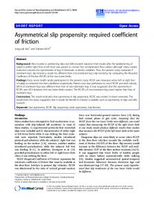
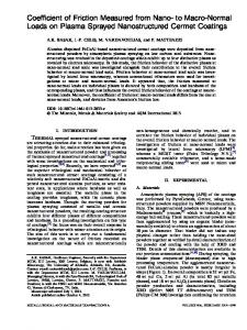
2.2 Slope Tests Slope tests are simple tests. They come with 2 variants, the sloped (micro)duct and the sloped cable test. They are easy to construct and are also available on the market [4]. 2.1.1 Sloped (micro)duct. In this test a (micro)duct sample, in which a short cable sample is placed, is mounted straight on a clamping device. The angle α with the horizontal at which the cable starts sliding is measured. The COF f simply follows from:

f = tan(α )

cable

This test is used for smaller types of cable, like microduct cables.

2.3 Bullet Test

(2)

A brass slider is shot through a curved piece of (micro)duct and the speed difference between two points is measured. This test is described in [5]. After analysing the forces it turns out that the sidewall forces fall outside the window of (A7) of Appendix A. The test, with its brass slider, is not suitable to distinguish between different constructions of cable or fibre unit.

3. Test Results Existing Test Methods

A: duct fixing strap B: duct C: setting wheel D: cable or fibre E: coefficient of friction indicator

Wheel tests are expected to give the right values for the COF, when using the proper weights, eliminating small diameter pulleys and using the right formula’s. Also slope tests, when using the proper weight around the (micro)duct sample in the sloped cable test, give those expectations. Users of said tests also claim good correlation between the measured COF and the blowing performance. However, the comparison found for different cable and (micro)duct samples (next paragraph), with different lubrication procedures, does not always show good correlation. Here the COF’s calculated from blowing reference tests can be much higher than measured with the wheel test described in this paper, see Figure 4 and text in next paragraphs. For this reason a decision was taken in IEC 86A WG3 not to incorporate tests to measure the COF in standards, but to write a separate technical document. Tests to measure the COF have been done on different 3.9 mm cables and 7 mm microducts (different suppliers) with the wheel test described in this paper. The microducts as received from the supplier were either dry, with low-friction liner or pre-lubricated. Tests have been performed with or without additionally lubricating the microducts with Jetting Lub [9] before blowing.

F: level indicator G: level setting screw H: blocking wheel I: base plate J: duct support

Figure 2. Sketch of the sloped (micro)duct test. Care shall be taken that the length of the piece of cable is small enough. The (intrinsic) bend radius of the cable shall not result in touching opposite walls of the (micro)duct, which would result in


414


mounted in the flow path. This equalizes the pressure when the cable is moved and air is pushed aside. Also it minimizes the effect of friction caused by the intrinsic curvature of the cable, an end effect disturbing the measurement.

COF calculated from blow ref test

0,6

0,5

L cable

0,4

pi

pe

F

0,3

airflow

0,2

microduct

Figure 5. Sketch of the blow simulation test. 0,1

0 0

0,1 0,2 Measured COF (w heel)

0,3

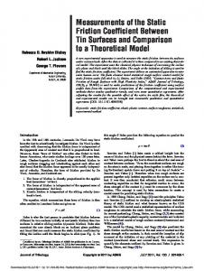
Figure 4. Calculated COF’s, from blowing reference tests of different cables in different microducts, plotted against measured COF’s (wheel test). The line represents 100% correlation. Blowing reference tests have also been performed. They were done in a trajectory of about 1500 m long with loops of 125 m long and in between them 180-degree bends of 0.25 m radius. The blowing pressure is maintained at 10 bar and the experiment is stopped when the blowing speed drops below 20 m/min. The COF has been calculated from the blowing distance, using Draka software which takes into account the filling of the duct by the cable (needed to obtain realistic COF-values when not reaching the duct-end, see Appendix B). Since this software cannot handle the separate bends this is simulated by windings with amplitude of 10 cm and period of 5 m (same result as for 180-degree bends of 0.25 m radius every 125 m, according to JETplanner [4]).

Figure 6. Picture of the pressure chamber of the blow simulation test. A Picture of the pressure chamber is shown in Figure 6. In Figure 7 the half of the test length is shown. The length extends in another room, through the wall. The total (micro)duct test length is 17.1 m. On the left side in Figure 7 a pneumatic extension can be seen, for the movement of the cable.

No points have been found under the line in Figure 4. This means that combinations of cables and microducts never perform better in blowing than what follows from the COF measured with the wheel test. But, many combinations perform less than what follows from the wheel test, especially the ones with the microducts which have not been additionally lubricated. For the well-performing combinations the correlation with blowing reference tests is rather good. Test methods to guarantee good blowing performance should also measure the effects of tacky lubricants and non-straight cables having little space. This can only be done with blow simulation.

4. Blow Simulation Apparatus A sketch of the blow simulation test is given in Figure 5. A sample cable is placed in a sample (micro)duct of length L. Air is forced to flow through the (micro)duct via a pressure chamber. The pressure and flow are controlled such that pressures pi and pe are maintained at the inlet and exit of the sample duct, respectively. The pressures and the flow are monitored. In the pressure chamber the cable is attached to a force sensor and moved back and forth (speed about 20 m/min), while monitoring the force. At the end of the sample duct a piece of a larger duct is


Figure 7. Half of the test length (rest through wall).

415


Here µ is the dynamic viscosity of the flowing medium (1.8×10-5 Pas for air) and ρa its density at atmospheric pressure (1.3 kg/m3 for air), Dh the hydraulic diameter (Dd with correction when filled with cable, see Appendix B) and pi and pe the pressures at the inlet and exit of the length L, respectively (note that Re is constant over the entire length of a duct when its hydraulic diameter is constant). It follows that exact copies of both forces on the cable and flow properties can only be obtained by cutting out windows from Figure 8. The relation between pi and pe is then found using (3):

5. Blow Simulation Theory When blowing a cable with pressure p0 the pressure p as a function of position x over the length l is given by [1,2]: p=

(

p 02 − p 02 − p a2

) xl

(3)

Here pa is the (atmospheric) pressure at the end of the (micro)duct. The pressures are given as absolute pressures. The net force dF/dx on a piece dx of the moving cable, which is the blowing force minus the friction force, is given by [1,2]: dp dp dF = − π4 Dd Dc ± fW ≡ −C blow ± fW dx dx dx

(4)

Re = 2.9

µ

2 2   ρ a pi − p e  2 Lp a 

   

)

(6)

For a moving cable in a straight length L, on which the pressure drop can be approximated linearly, and for a tensile force on the cable (F positive), the COF follows from (4):

Here W is the weight of the cable per unit of length, f is the COF between cable and (micro)duct and Dd and Dc are the inner diameter of the (micro)duct and outer diameter of the cable, respectively. For forward movement the sign of the friction force is negative, for backward movement positive, while a tensile force is positive. The pressure, blowing force and friction force on the cable are given in arbitrary units in Figure 8. Here the friction force is also given, at the same scale as the blowing force, for a typical jetting (synergy of blowing and pushing) installation. In a blow simulation test the parameters are chosen the same as in the blowing reference test. Take samples of the cable and the (micro)duct and copy the lubrication process (if any). Then choose the same conditions for the airflow. The length L of the samples shall be large enough that onset of the flow occurs at a relative short length and the flow can be considered as “fully developed”. Also the Reynold number Re shall be the same as in the practical installation. For turbulent flow (Blasius equation) this number follows from [1,2]: Dh12 / 7 8/ 7

(

L 2 p 0 − p a2 l

p i2 − p e2 =

π

4

f =±

D d Dc ( p i − p e ) − F

(7)

WL

Here the positive sign represents forward movement and the negative sign backward movement. During forward movement the force may also be compressive (when the friction forces are higher than the air propelling forces). In this case f is found numerically. When the air propelling factor Cblow is indeed given by the theoretical expression from (4) the COF found for forward and backward movement will be the same. If the air propelling force is also influenced in another way, e.g. by a textured surface on the cable, different and hence wrong results are found. In this case the factor Cblow shall be regarded as unknown. From the 2 equations (one for forward and one for backward) the 2 unknowns f and Cblow are found: f =

4/7

(5)

Fb − F f

(8)

2WL

C blow =

Fb + F f

(9)

2( p i − p e )

Here Ff and Fb are the forces measured in forward and backward movement, respectively.

p

pi pe

6. Test Results Blow Simulation

- C blow dp dx

L

The blow simulation tests have been performed on 7, 10 and 12 mm microducts (one supplier) with different cable types at pressures as listed in Table 1. They represent “windows” of 17.1 m on a 1ength l of 1500 m and a pressure p0 of 10 bar at the beginning of this length, pi and pe obtained with Equation (6). In Table 1 also the relative positions x/l have been given of these “windows”.

window

Table 1. Pressures for 7, 10 and 12 mm microducts

fW 0

l

Figure 8. Pressure p, blowing force Cblow × dp/dx and friction force fW as a function of the position in a duct of length l in a blowing reference tests. Windows of length L, with pressure pi and pe at inlet and exit, respectively, are taken for the blow simulation test.


x/l

0.45

0.60

0.75

0.90

1.00

pi (bar)

7.18

6.00

4.56

2.61

0.54

pe (bar)

7.10

5.90

4.44

2.41

0.00

The samples were taken from blowing reference tests. From these tests the COF was calculated in the same way as those from Figure 4. The results from the field tests and the blow simulation tests are given in Figure 9. Microducts with too little (none) or too much lubricant (Microlub or Jetting lub [9]) were also used, by purpose, to get more information about the validity of the blow simulation test.

416



0,5

The blow simulation tests also gives information about the air drag force. This force usually varies between the same as resulting from the existing blowing theory [1,2] and 10% more. No significant correlation of the air drag force and the roughness of either the cable or the (micro)duct has been found in our experiments. Bearing in mind that changing either the roughness of the cable or the (micro)duct (grooves) has in some cases led to increased blowing performance (much more than 10%) leads to the conclusion that this had affected rather the COF than the air drag force. The blowing theory is therefore confirmed as a good tool to forecast blowing performance.

0,4

0,3

0,2

The blow simulation test has helped in the further improvement of the microduct cabling and their installation. One such development is the cable lubricator [11], see Figure 11. The use of this apparatus corresponds to the most left point in Figure 9 (COF of 0.06, really effective now; note that such a value was measured often in a wheel test). Not only the 1500 m blowing reference test could be done at low pressure, also a new record in microduct cabling was achieved: at CERN [12] a 24 fibre cable (3.9 mm) was recently blown with the help of the cable lubricator into a 7/5.5 mm microduct over a length of 3.5 km (in one shot!).

0,1

0 0

0,1 0,2 0,3 0,4 Measured COF (sim ulation)

0,5

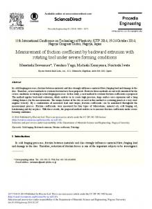
Figure 9. Calculated COF’s, from blowing ref. tests of different cables in different microducts, plotted against measured COF’s with the blow simulation test. The line represents 100% correlation. In Figure 10 the results are given of the wheel tests, from the same samples as from Figure 9. Clearly there is little correlation between the measured COF here and the COF obtained from the blowing reference tests, while the blow simulation test showed excellent correlation in Figure 9. The small deviations in Figure 9 were attributed to not constant lubrication over the length of the blowing reference tests, as was observed by performing blow simulation tests on samples taken from different locations. A blow simulation reference test only gives one (average) value for the COF, while in the blowing reference tests the different local values are found.


0,5

0,4

0,3

0,2

Figure 11. Cable blowing equipment (blue apparatus) and cable lubricator (red apparatus) at work during one-shot 3.5 km blowing of a 24-fibre cable into a 7/5.5 mm microduct at CERN.

0,1

7. Conclusions

0 0

0,1

0,2 0,3 0,4 Measured COF (w heel)

It is concluded that existing techniques to measure the COF between cable and (micro)duct, such as the wheel test, do not offer sufficient reliable values to guarantee good blowing performance. An alternative test, the blow simulation test, has been described in this paper. Here a cable moves backward and forward in a microduct with airflow, simulating a window in a real installation (when moving forward). The measured forces supply information on both friction and air drag force. Measurements show excellent correlation with blowing. The air drag force is the same or 10% more than

0,5

Figure 10. Calculated COF’s, from blowing reference tests of different cables in different microducts, plotted against measured COF’s with the wheel test. The samples are the same as used for Figure 9. The line represents 100% correlation.


417


would result from the existing blowing theory, confirming this theory.

Hydrodynamic or “thick-film” friction is significant on sections with low sidewall bearing pressure between cable and duct. Under these conditions the cable actually floats on a “thick” film of lubricant. The viscosity of the lubricant (low for low friction of this type) plays an important role. This type of friction also increases at higher cable speeds.

8. Acknowledgments Special thanks to Willie Greven, Thomas Pothof, Frans Bakker, Ate de Jong and Cees van ‘t Hul (Draka Comteq Telecom B.V.) for performing the blowing reference tests, and to Arie van Wingerden, Arnie Berkers and Dick Huisman (Draka Comteq Telecom B.V.) for the supply of (special) cables. Also acknowledged are John Fee (Polywater Inc.) and Gerard Plumettaz (Plumettaz S.A.) for their stimulating discussions. Finally acknowledged are Ted Sugito (Draka Comteq Telecom B.V.), Luit de Jonge (CERN), Philippe Pache, Tony Garcia and crew (Mauerhofer & Zuber) for the 3.5 km one shot blowing.

Boundary or “thin film” friction is significant on sections with high sidewall bearing pressure between cable and duct. Under these conditions lubricants get squeezed into a thin film and may break down and loose effectiveness. This type of friction is also dominant when no lubricants are used. With cable blowing both types of friction may occur, depending on cable weight, forces in the cable, cable speed, lubricant used and bend radii in the duct trajectory. It is important that the conditions in the COF measurement are as close as possible to those in the actual blowing situation.

9. References [1] W. Griffioen, ”Installation of optical cables in ducts, Plumettaz, Bex (CH) 1993. [2] W. Griffioen, "The installation of conventional fibre optic cables in conduits using the viscous flow of air", J. Lightwave Technol., Vol. 7, no. 2 (1989) 297. [3] IEC 60794-1-1, Annex C, “Generic specification for optical fibre cables”, edited 2004. [4] JETplanner and slope test equipment, Plumettaz, Bex, Switzerland, www.plumettaz.ch. [5] D. Butler, D.J. Stockton, “Duct surface testing for use in optical fibre transmission lines”, Patent application GB2205960A (1987). [6] IEC 60794-5, “Sectional specification for microduct cabling for installation by blowing”, Committee Draft from SC 86A WG3. [7] W. Griffioen, A. van Wingerden, C. van 't Hul, M. Keijzer, "Microduct cabling: Fiber to the Home", Proc 52nd IWCS (2003) 431-437. [8] J.M. Fee, S.H. Dahlke, D.P. Solheid, “Analysis and measurement of friction in high speed air blowing installation of fiber optic cable”, Presented at the National Fiber Optic Engineers Conference, June 18-22, 1995, Boston, MA. [9] Jetting Lub and Microlub, Polywater, Stillwater, Minnesota, www.polywater.com and Plumettaz, Bex, Switzerland, www.plumettaz.ch. [10] G.C. Weitz, “Prediction and minimization of fiber optic pulling tensions”, IEEE Journal of Selected Areas in Communications, vol. sac-4, no. 5, 1986, pp. 686-690. [11] Optical cable installation with cable lubricator, United State Patent US 6,848,541, Feb. 1, 2005. [12] W. Griffioen, C. van ‘t Hul, I. Eype, T. Sugito, W. Greven, T. Pothof, R. Khiar, L.K. de Jonge, “Microduct cabling at CERN”, Proc 53rd IWCS (2004) 204-211.

Another contributor to friction is the effect of static electricity. This is especially important for the very low weight “cables”, like microduct fibre units. This effect depends strongly on speed and also on environmental conditions as present with blowing. It is extremely difficult to test this effect in ways other than blowing tests. Finally the effect of wear of cable and duct on friction during installation are mentioned. While this phenomena occurs with cable pulling it is hardly present with cable blowing, where forces involved are an order of magnitude smaller. The actual friction is not only determined by a pure COF and the other parameters following from blowing theory and used in planner software [4]. Other effects also play an important role, like non-straightness or memory of the cable or microduct, squeezing the cable between the inner walls of the microduct by their own “spring action”, especially when the diameter of the cable is relatively large. This effect is also measured in some tests, like an effective COF, but most tests do not measure this.

A2. Forces during Blowing One of the important factors mentioned in the previous section is the sidewall bearing pressure between cable and (micro)duct. This is best expressed in sidewall (normal) force Fn. Often a much higher sidewall force is used in a measurement of the COF than is present in an actual blowing situation. For blowing in a straight (micro)duct the sidewall force is simply the weight of the cable. For a cable with weight W per unit of length and length l this is: Fn = Wl

In a bend with radius Rb in the duct trajectory the sidewall force depends on the longitudinal force F in the cable: Fn =

Appendix A: Analysis of Friction In an experiment to measure the COF the conditions during the actual blowing need to be approximated as much as possible. In order to indicate which parameters are important, and which boundary conditions need to be taken for them, a short analysis of friction will be given in this appendix.

F l Rb

(A2)

Usually the length of a bend is shorter than the length in the measurement of the COF, especially for sharp bends in the trajectory, so the force found in this formula gives the upper limit of effective sidewall force. The force can be tensile or compressive, both resulting in an absolute positive value for the sidewall force. In blowing usually compressive forces dominate, especially short after the installation equipment. A typical value of the pushing force used for blowing is:

A1. Friction Contributors In most cases lubricants are used to reduce friction between cable and duct. Two types of friction can be distinguished: hydrodynamic friction and boundary friction [10].


(A1)

418


F push = W × 500m

with (following with Blasius equation [1,2]):

(A3)

However, the pushing force rapidly decreases more than an order of magnitude short after the installation equipment [1,2] and the COF in this high pushing force section does not count significantly to the total blowing length that can be reached. Most important for the blowing performance is the part where blowing forces are about equal to the friction. And here again (A1) holds.

p ch =

π 4

Dc Dd ∆p

(A4)

For longitudinal extending flow channels, not deviating too much from cylindrical, the hydraulic diameter Dh is defined as 4 times the wetted area divided by the wetted surface of the cross-sectional area. For a (micro)duct with cable then simply follows:

Here Dc and Dd are the diameters of the cable and the (inner) duct and ∆p is the pressure drop over a duct section. Since airpropelling forces built-up at one section can only reach sections not too far away, because of friction, only a part of the pressure drop of the total is effectively contributing to the cumulative blowing force. Also a part of the cumulative blowing force is already used for compensation of friction in the section where it is built-up. A good approximation of the excess cumulative blowing force that can be generated (in a trajectory of about the maximum blowing length) is obtained by using (A4) with a pressure drop of about 0.5 bar (this can be the drop over 200 m) for the excess blowing force. For a constant filling rate of (micro)duct with cable the blowing force is proportional to the square of the cable diameter and hence proportional to the cable weight (for a constant cable density). For a typical microduct cable in a microduct this results, using the previous information, in an excess blowing force: Fblow,excess = W × 5m

D h = D d − Dc

p i2 − p e2 µ 1 / 4 ρ a3 / 4 7 / 4 = 0.24 Φa 2 Lp a Dd19 / 4

(

Dd19 / 4 ⇒ Dd2 − Dc2

 D Dh = Dd 1 −  c   Dd 

(A7)

Appendix B: Calculate COF from blowing In order to calculate the COF from blowing experiments where the cable does not reach the duct end it is needed to know the effect of filling of the (micro)duct with cable, i.e. the effective hydraulic diameter Dh as appearing in (5).

(

) xx

Dh5 / 4

(B5a)

   

2

  

−7 / 5

Φf  Φ  e

   

7/5

(B6)

Taking into account only the data in the turbulent regime the flow in the empty microduct is up to 15 % higher than following from (B5). This is not unusual. Blasius’ equation is valid for smooth walls. Surface roughness will decrease the flow and longitudinal ribs (as is the case with the tested microduct) may increase the flow, due to directing effects of the ribs on the flow. From (B6) an hydraulic diameter Dh is found of 0.4 Dd. This is a little higher than what follows from (B3).

Equation (3) is valid for a flow channel of uniform (hydraulic) diameter, e.g. an empty (micro)duct or a (micro)duct entirely filled with cable. When the cable gets stuck somewhere underway this is not the case anymore. Now (3) needs to be replaced by the expression for the pressure over the cable, until the pressure pch at the location xch of the cable head: 2 p 02 − p 02 − p ch

7/4

In Figure B1 an example is given for a 7/5.5 mm microduct of 19 m. The flow is measured as function of the inlet pressure while the exit pressure is atmospheric, for an empty microduct and for a microduct filled with a 3.9 mm cable. The effect of filling can be clearly seen. Also the transition from laminar to turbulent flow can be seen for the filled microduct. The present blowing theory is not valid for laminar flow. Fortunately both practical installation of microduct cables (e.g. 1500 m with 10 bar) and the resulting blow simulation friction measurements (pi of 0.59 bar for pe = 0 and L = 19 m) occur in the turbulent regime.

Together with the condition (A1) for straight duct sidewall force this results in the following window for the normal force per unit of length in a COF measurement for microduct cabling:

p=

)

From measuring the flow Φf for the filled and then the flow Φe for the unfilled (micro)duct (both under atmospheric conditions), at the same pressures, the hydraulic diameter can then be obtained with:

(A6)

Fn ≤ 10W l

(B5)

Here the volume flow Φa is defined at atmospheric conditions. For a filled (micro)duct (B5) is valid with the following replacement:

This excess force is much more relevant for the blowing length that can be reached than the force from (A3). Microducts are usually not bent sharper than with a radius of 0.5 m over the trajectory (sometimes a sharper bend at a branch location). Hence for microduct cabling (A2) and (A5) result in:

W≤

(B3)

However, the situation of a (micro)duct filled with cable appears to be too far away from the cylindrical case and (B3) does not give the right result. Fortunately the effective hydraulic diameter can be obtained from measuring the flow through the (micro)duct when empty and when filled. For turbulent flow (Blasius equation) [1,2] it follows, for an empty (micro)duct:

(A5)

Fn = 10Wl

(B2)

This effect of filling the (micro)duct with cable only counts for ducts with high filling degree (such as is often the case with microduct cables) and when the cable does not reach the end. Draka has developed jet-planning software that takes this filling into account. Using this software the COF can be calculated from blowing experiments using (micro)ducts with fixed length where not always the end is reached. This COF can than be compared to the COF from the friction or blow simulation experiments.

Because of expansion of the air the blowing force is not equally distributed over the duct length. Hence longer cable sections can experience a mismatch between friction and compensation by airpropelling forces. The cumulative blowing force given by [1,2]: Fblow =

(l − xch ) p02 (Dd2 − Dc2 )7 / 4 Dh5 / 4 + xch p a2 Dd19 / 4 (l − x ch )(Dd2 − Dc2 )7 / 4 Dh5 / 4 + xch Dd19 / 4

(B1)

ch


419


Sito Zandberg attended the Hogere Technische School in Leeuwarden where he received a B.Sc. in Chemical Engineering in 1982. After he fulfilled his duty in the Dutch Army he joined the Dutch Oil Company NAM as a Drilling Fluid Engineer. Here he worked on the improvement of the solid removal system of drilling rigs. In 1987 he joined Draka Comteq as a production engineer. In 1992 he became head of the laboratory that checks all incoming goods. At the moment he works as a Production Material Engineer and is responsible for new materials for cables, trouble shooting if there are processing problems and testing of microducts, cables and COF measurements. Draka Comteq Telecom, IJzerweg 2, 9936 BM Farmsum.

0.8

flow (ml/s)

empty

0

filled

0

p i (bar)

0.6

Figure B1. Flow as a function of inlet pressure pi (zero at exit) of a 7/5.5 mm microduct of 19 m. Square symbols represent an empty microduct, circle symbols the microduct filled with a 3.9 mm cable. Gray symbols indicate laminar flow.

Biographies Willem Griffioen received an M.Sc. degree in Physics and Mathematics from Leiden University (Netherlands) in 1980 and worked there until 1984. He joined KPN Research, St. Paulusstraat 4, 2264 XZ Leidschendam, The Netherlands. Responsibilities R&D of Outside-Plant and Installation Techniques. He worked at Ericsson Cables, Hudiksvall (Sweden) and at Telia Research, Haninge (Sweden) in the scope of exchange/joint projects with KPN Research. He received his Ph.D. (Reliability of Optical Fibers) in 1995 from the Technical University of Eindhoven (Netherlands). Currently, since 1998, he is product manager at Draka Comteq Telecom, Zuidelijk Halfrond 11, 2801 DD Gouda, The Netherlands.


Menno Versteeg attended the Leidse Instrumentmakers School (metal 1989) at Leiden. In 1997 he received his B.Sc. degree in Applied physics (Photonics). Also in 1997 he fulfilled his duty to the Dutch Army as a Medical Engineer (N39XO), he was responsible for checking, repairing and setup of the all medical equipment being used by the Dutch Army. He has worked at ESAESTEC (1995), Fokker Space (1996) and TNO-TPD (1998) as Head of Technical Support in the Optical Components and Thin Layers Department. During the above he gave technical support in optical systems of different satellite components (GOME and OMI). Currently, since 2001, he is System Engineer at Draka Comteq Telecom - Zuidelijk Halfrond 11, 2801DD, Gouda, The Netherlands. Maja Keijzer received a BSc degree, a MSc degree, and PhD in Chemical Engineering respectively in 1990 (The Hague), 1993 (Eindhoven) and 1998 (Delft) on polymer science, (in)organic chemistry, electro-chemistry and corrosion protection. She worked at Netherlands Energy Research Foundation ECN as project leader on material development for solid polymer fuel cells. In 2001 she joined Draka Comteq Telecom as product manager. Currently, since 2003, she works as Technical Manager on corrosion protection at Vecom Metal Treatment B.V., Mozartlaan 3, 3144 NA Maassluis, The Netherlands.

420
