An excellent discussion on data modeling and optimization can be found in ..... a stochastic approximation method, evolution algorithms, a multiple-level single-.
1.7 Parameter Optimization and Nonlinear Fitting JIÌÍ ŠIMæNEK, George E. Brown, Jr. Salinity Laboratory, USDA-ARS, Riverside, California JAN W. HOPMANS, University of California, Davis, California
1.7.1 Introduction Experimentalists often collect data that later need to be summarized to infer or investigate cause–effect relationships. The data sets and derived relationships can be either static or dynamic. Soil water retention data (relating soil water matric head with soil water content; Section 3.3) or hydraulic conductivity data (relating unsaturated hydraulic conductivity with soil water matric head or water content; Section 3.5) represent typical examples of such data sets. The data can be expressed in a graphical form by simply drawing an eye-balled curve, or in functional form by fitting a curve from a selected class of functions through the data. The fitting process is called curve fitting or model fitting, depending on whether an arbitrary or theoretically derived function was selected to describe the behavior of the physical and/or chemical system under observation. For example, fitting a soil water retention curve (e.g., van Genuchten’s [1980] equation) can be considered as curve fitting since the equation is almost completely empirical, whereas fitting a solute breakthrough curve can be viewed as a model fitting process if the fitted function is an analytical solution of the convection–dispersion equation (see Sections 6.3 and 6.5). Alternatively, fitting the van Genuchten–Mualem unsaturated hydraulic conductivity function (van Genuchten, 1980) is a combination of curve and model fitting since the conductivity function is derived theoretically from a pore-size distribution model, but uses an empirical retention function. Although, in principle, curve and model fitting are not much different, curve fitting is more arbitrary. One typically selects an arbitrary function and the best-fit criterion is often formulated independent of statistical considerations (Bard, 1974). For model fitting, the functional relationship is well defined and only the parameters are unknown. Thus, functions obtained from curve fitting summarize the available data without necessarily increasing insight into the nature of observed processes and are generally limited to the measurement range. The process of model fitting is closely related to parameter estimation. Theoretically derived models (i.e., relationships describing a particular physical process) include parameters that describe physical properties of the observed system (e.g., the saturated hydraulic conductivity, porosity, diffusion coefficient, cation exchange capacity, infiltration rate, or others). Hence, one would expect that fitting 139
140
CHAPTER 1
a correct model produces estimated parameters that describe these physical properties with a certain accuracy. Consequently, the results of model fitting can often be extrapolated to beyond the measurement range. By comparison, parameters obtained by curve fitting generally have little or no physical significance. A simple case of curve or model fitting arises when fitting a functional relationship between a dependent variable y and a set of n variables xi, i = 1,..., n. A more complex problem arises when the fitting model is represented by one or more differential equations, with the measured variables representing either primary or secondary variables (the latter being derived from the primary variables). A typical example of such a problem involves the transient variably saturated water flow equation. The model is represented by the Richards equation, while the measured variables are matric heads and/or water contents (primary variables), or water fluxes and the sample soil water storage (secondary variables). To match the model with experimental variables, selected parameters in the soil hydraulic properties are usually fitted to functional relationships. In this section we briefly describe the process of parameter estimation. We include a discussion on least-squares and maximum-likelihood estimators, minimization techniques, significance of optimized parameters and their confidence intervals, and goodness of fit. Readers interested in more details are encouraged to study the texts of Bard (1974) and Beck and Arnold (1977), among many others. Detailed descriptions of proven experimental techniques that utilize parameter estimation to estimate soil hydraulic and transport properties are presented in Sections 3.6.2 and 6.6, respectively. 1.7.2 Maximum-Likelihood and Weighted Least-Squares Estimator The general approach in model fitting is to select a merit or objective function that is a measure of the agreement between measured and modeled data, and which is directly or indirectly related to the adjustable parameters to be fitted. The best-fit parameters are obtained by minimizing (or maximizing, depending on how the function is defined) this objective function. If no model and measurement errors exist, this minimum value would be zero. However, even if the model is perfect, experimental errors will generally create a non-zero minimum value for the objective function. An excellent discussion on data modeling and optimization can be found in Press et al. (1992). When measurement errors follow a multivariate normal distribution with zero mean and covariance matrix V, the likelihood function can be written as (Bard, 1974) β) = (2π)−n/2(detV)−1/2exp{(−1/2)[q* − q(β β)]TV−1[q* − q(β β)]} L(β
[1.7–1]
β) is the likelihood function, β = {β1, β2,..., βm} is the vector of optimized where L(β parameters, m is the number of optimized parameters, q* = {q*1, q*2,..., q*n} is a vecβ) = {q1, q2,..., q*n} is the corresponding vector of model pretor of observations, q(β dictions as a function of the unknown parameters being optimized, and n is the number of observations. The differences between measured and computed quantities, β), are called residuals. The likelihood function L(β β) is defined as the joint q* − q(β probability density function of the observations and identifies the probability of the
SOIL SAMPLING AND STATISTICAL PROCEDURES
141
data, given the parameter vector β (Bard, 1974). The maximum-likelihood estimate is that value of the unknown parameter vector β that maximizes the value of the likelihood function. Since the logarithm is a monotonically increasing function of its β) also maximize argument, the values of β that maximize the likelihood function L(β β). This property of the logarithm is frequently used in parameter identificalnL(β tion studies since lnL is a simpler function than L itself. Hence, Eq. [1.7–1] is reformulated as the log-likelihood or support criterion (Carrera & Neuman, 1986a) β) = −(L*/2) = −(n/2) ln(2π) − (1/2) ln(detV) ln L(β β)]T V−1 [q* − q(β β)] − (1/2) [q* − q(β
[1.7–2]
The notation of L* is used in Section 1.7.5. The maximum of the likelihood function must satisfy the set of m β-likelihood equations β)]/∂βi = 0 [∂ln L(β
i = 1,...., m
[1.7–3]
If all elements of the covariance matrix V are known, then the value of the unknown parameter vector β which maximizes Eq. [1.7–3] must minimize Φ: β) = [q* − q(β β)]TV−1[q* − q(β β)] Φ(β
[1.7–4]
which constitutes the last term of Eq. [1.7–2]. If information about the distribution of the fitted parameters is known before the inversion, that information can be included in the parameter identification procedure by multiplying the likelihood function by the prior probability density funcβ), which summarizes this prior information. Estimates that make use of tion, p0(β prior information are known as Bayesian estimates, and lead to the maximizing of β), given by a posterior probability density function, p*(β β) = cL(β β)p0(β β) p*(β
[1.7–5]
in which c is a constant that insures that the integral of the posterior probability density function is equal to one. The posterior density function is proportional to the likelihood function when the prior distribution is uniform. Inclusion of prior information leads to the following expression to be minimized β) = [q* − q(β β)]TV−1[q* − q(β β)] + (β β* − β)TVβ−1(β β* − β) Φ(β
[1.7–6]
where β* is the parameter vector containing the prior information and Vβ is a covariance matrix for the parameter vector β. The first term in Eq. [1.7–6] penalizes for deviations of model predictions from measurements, while the second term penalizes for deviations of parameter estimates β from the prior estimate of the parameters β*; this prior estimate may be viewed as a reasonable first guess of β (McLaughlin & Townley, 1996). The second term of Eq. [1.7–6], also called the penalty function, ensures that the obtained parameter estimate is constrained to a physically meaningful range of values. The solution of the minimization problem,
142
CHAPTER 1
Eq. [1.7–6], is a compromise between the best-fit estimate associated with minimization of the first term, and the prior estimate associated with the second term (McLaughlin & Townley, 1996). Russo et al. (1991) showed that the use of a penalty function can significantly improve the uniqueness of the estimated parameters. The covariance matrices V and Vβ are also referred to as weighting matrices and provide information about measurement accuracy and correlation between measurement errors, V, and between parameters, Vβ (Kool et al., 1987). When the covariance matrix V has only non-zero diagonal elements, then the measurement errors are uncorrelated. No prior information about the optimized parameters exists if all elements of Vβ are equal to zero. In that case, the problem simplifies to a weighted least-squares problem β) = Φ(β
n
Σ wi[q*i − qi(ββ)]2 i=1
[1.7–7]
where wi is the weight of a particular measured point. The weighted least-squares estimator of Eq. [1.7–7] is a maximum-likelihood estimator as long as the weights, wi, contain the measurement error information such that wi = 1/σ2i = 1/variance of measurement error of q*i
[1.7–8]
However, in many applications, the measurement errors are either unknown or weights are not specified based on probabilistic assumptions. It is then difficult to interpret the resulting optimized parameters, their confidence intervals, correlations, and in general their relationship with the true parameter values (Bard, 1974). Weights significantly affect the shape and the absolute values of the objective function, and when selected arbitrarily, this arbitrariness is reflected in all subsequent statistical evaluations given in Sections 1.7.4 and 1.7.5. Improper selection of weights can influence not only the confidence regions of optimized parameters, but also the location of the minimum of the objective function (Hollenbeck & Jensen, 1998). The robustness of the least-squares criterion for the estimation of model parameters has recently been questioned by Finsterle and Najita (1998). They pointed out that the least-square criterion causes outliers to strongly influence the final values of optimized parameters. Hence, outliers (e.g., individual data points with large measurement errors, as is often the case with field measurements) can introduce a significant bias in the estimated model parameters. Finsterle and Najita (1998) studied several other more robust estimators with different error distributions that reduce the effect of outliers on the optimized parameters. For example, they suggest use of the least absolute deviates or L1 estimator if errors follow a double exponential distribution: β) = Φ(β
n
Σ (1/σi)|q*i − qi(ββ)| i=1
[1.7–9]
and the maximum-likelihood estimator for measurement errors that follow a Cauchy distribution:
SOIL SAMPLING AND STATISTICAL PROCEDURES
β) = Φ(β
143
n
Σ log{1 + (1/2)wi[q*i − qi(ββ)]2}
i=1
[1.7–10]
Still other estimators that do not correspond to any standard probability density function were suggested by Huber (1981) and Andrews et al. (1972). Robust estimators decrease the relative weights of outliers and thus make the estimated parameters less affected by the presence of random errors following a heavy tailed distribution (Finsterle & Najita, 1998). Uniqueness, identifiability, stability, and ill-posedness are terms often encountered in the parameter estimation literature. Since exact definitions and detailed discussions of these terms were given by Carrera and Neuman (1986b), we will only present a brief definition of each. The solution is said to be nonunique whenever the minimization criterion (i.e., the objective function) is nonconvex, that is, has multiple local minima or the global minimum occurs for a range of parameter values. The convexity of the objective function can be enhanced by inclusion of prior information, Eq. [1.7–6], in the analysis. The parameters are nonidentifiable when different combinations of parameters lead to a similar system response, thereby implying that a unique solution is impossible. Stability is achieved if the optimized parameters are insensitive to measurement errors, that is, small errors in the system response must not result in large changes in the optimized parameters. Finally, the inverse problem is ill-posed if the identified parameters are unstable and/or nonunique. Inverse problems used to estimate parameters of the unsaturated soil hydraulic functions are often ill-posed, but can become well-posed in case of welldesigned experiments for homogeneous soils with small measurement and model errors (Hopmans & Šimçnek, 1999). An ill-posed problem can be replaced by a wellposed problem by adding more or other type of measurements, and/or by constraining the value range of the set of adjustable parameters. 1.7.3 Methods of Solution Many techniques have been developed to solve the nonlinear minimization or maximization problem (Bard, 1974; Beck & Arnold, 1977; Yeh, 1986; Kool et al., 1987). Most of these methods are iterative by requiring an initial estimate β i of the unknown parameters to be optimized. The behavior of the objective function, β), in the neighborhood of this initial estimate is subsequently used to select a Φ(β direction vector v i, from which updated values of the unknown parameter vector are determined, that is, β i+1 = β i + ρ iv i = β i − ρ iRipi
[1.7–11]
The direction vector is computed so that the value of the objective function decreases, or Φi+1 < Φi
[1.7–12]
where Φi+1 and Φi are the objective functions at the previous and current iteration level, Ri is a positive definite matrix, pi is the gradient vector, and ρ i is the step size.
144
CHAPTER 1
Methods based on Eq. [1.7–11] are called gradient methods. The various gradient methods used in the literature (e.g., steepest descent, Newton’s method, directional discrimination, Marquardt’s method, the Gauss method, variable metric methods, and the interpolation–extrapolation method) differ in their choice of the step direction, vi, and/or the step size, ρ i (Bard, 1974). The steepest descent method uses ρ i = 1 and Ri = I, where I is an identity matrix. The Newton method uses ρi = 1 and β): Ri = H−1, where H is the Hessian matrix of Φ(β β) = (∂2Φ/∂βi∂βj) Hij (β
i, j = 1,...., m
[1.7–13]
The steepest descent method is often inefficient, requiring many iteration steps to reach the minimum, and consequently is not recommended. The Newton method is usually not recommended because it requires evaluation of second derivatives, thus making it computationally inefficient, especially for problems involving solution of partial differential equations. The Gauss–Newton method simply neglects the higher-order derivatives in the definition of the Hessian matrix and assumes that H can be approximated by a matrix N using only the first-order derivatives. For nonlinear weighted least squares this leads to H ≈N = JwT Jw
[1.7–14]
where Jw is the product of the Jacobian matrix J β)] β) ∂[qi* − qi(β ∂qi(β Jij = ____________ = − ________ ∂βj ∂βj
[1.7–15]
and the lower triangular matrix L of the Cholesky decomposition of V −1 (Jw = LJ). Marquardt (1963) proposed a very effective method, commonly called the Marquardt–Levenberg method, which has become a standard in nonlinear leastsquare fitting among soil scientists and hydrologists (van Genuchten, 1981; Kool et al., 1985, 1987). The method represents a compromise between the inverse-Hessian and steepest descent methods by using the steepest descent method when the objective function is far from its minimum, and switching to the inverse-Hessian method as the minimum is approached. This switch is accomplished by multiplying the diagonal in the Hessian matrix (or its approximation N), sometimes called the curvature matrix, with (1 + λ), where λ is a positive scalar, leading to H ≈ JwTJw + λDTD
[1.7–16]
where D is a diagonal scaling matrix whose elements coincide with the absolute values of the diagonal elements of the matrix N. When λ is large, the Hessian matrix is diagonally dominant, resulting in the steepest descent method. On the other hand, when λ is zero, Eq. [1.7–16] reduces to the inverse-Hessian method. A common strategy is to initially select a modest value of λ (e.g., 0.02) and then decrease its value as the solution approaches the minimum (e.g., multiply λ by 0.1 at each iteration step).
SOIL SAMPLING AND STATISTICAL PROCEDURES
145
The computationally most time-consuming part of both the Gauss–Newton and Marquardt–Levenberg methods is the evaluation of Jacobians. The sensitivity coefficients may be calculated using three different methods (Yeh, 1986): the influence coefficient method (finite differences), the sensitivity equation method, and the variational method. When using the influence method, one has to balance trunβ, with rounding errors that decrease with ∆β β. A cation errors that increase with ∆β common practice is to use a one-sided difference method, that is, to change the optimized parameters by 1% β + ∆β βej) − qi(β β) ∂qi qi(β ___ ≈ _______________ ∂βj ∆βj
[1.7–17]
β is the small increment of β (e.g., 0.01β β). With where ej is the jth unit vector, and ∆β a total number of m fitting parameters, the governing equation must be solved (m + 1) times during each iteration of the nonlinear minimization. A better estimate of the sensitivity coefficients can be obtained by using a central difference scheme β + ∆β βej) − qi(β β − ∆β βej) ∂qi qi(β ___ ≈ _____________________ ∂βj 2∆βj
[1.7–18]
However, since this scheme requires evaluation of the objective function for two additional parameter values for each optimized parameter, contrary to only a single evaluation for a one-sided difference scheme, the central difference approach is usually not recommended. Depending upon the problem being considered (e.g., measurement errors, number of optimized parameters, type of measurements), the objective function Φ may be topographically very complex without a well-defined global minimum and/or having several local minima in parameter space. The behavior of the objective function is often analyzed using contour plots of response surfaces. Specifically, the objective function is calculated for two selected perturbed parameters, while the other optimized parameters are kept constant, so that the contours can be graphically represented in a two-parameter plane. Contours of the objective function will reveal the presence of local minima, parameter sensitivity, and parameter correlation. Since a response surface analysis studies only cross-sections of the full parameter space, such an analysis can therefore only suggest how the objective function might behave in the full m-dimensional parameter space (Hopmans & Šimçnek, 1999). Minimization methods can be highly sensitive to the initial values of the optimized parameters. Depending upon the initial estimate, the final solution may not be the global minimum, but instead a local minimum. Consequently, when using gradient-type minimization techniques, it is generally recommended to repeat the minimization problem with different initial estimates of the optimized parameters and to select those parameter values that minimize the objective function. More robust minimization techniques have recently been used by Pan and Wu (1998), who used the annealing-simplex method; by Abbaspour et al. (1997), who used a sequential uncertainty domain parameter fitting (SUFI) method; and by Vrugt et al. (2001), who used a genetic algorithm.
146
CHAPTER 1
In recent years, the increased interest in robust minimization algorithms has led to global optimization techniques (e.g., Barhen et al., 1997) that uniquely search for the global minimum. These methods include fast simulated annealing, a stochastic approximation method, evolution algorithms, a multiple-level singlelinkage method, an interval arithmetic technique, taboo search schemes, subenergy tunneling, and non-Lopschitzian terminal repellers (Barhen et al., 1997), but have not yet, or only sparingly, been used for unsaturated zone flow and transport problems. 1.7.4 Correlation and Confidence Intervals Since parameter estimation involves a variety of possible errors, including measurement errors, model errors, and numerical errors, an uncertainty analysis of the optimized parameters constitutes an important part of parameter estimation. Parameter uncertainty analyses usually assume that the solution converges to a global minimum, and that the model error is zero, so that parameter uncertainty is limited to measurement errors only. A confidence region of the parameter estimates can then be defined exactly by using a maximum allowable objective function increment (from its minimum) β) − Φmin| ≤ ε |Φ(β
[1.7–19]
where Φmin is the best attainable value of the objective function Φ, and ε is the largest difference between risks that one is willing to consider as being insignificant (Bard, 1974). The set of values β that satisfies this equation is known as the ε−indifference region. If ε is sufficiently small so that Φ can be approximated by means of its Taylor series expansion, the indifference region has a typical m-dimensional ellipsoid-type shape. An exact confidence region for nonlinear problems can be obtained by contouring the objective function with reference to some fixed levels of confidence (ε). This procedure is rather computationally expensive, especially for problems involving numerical solution of partial differential equations, since it usually requires discretizing the parameter space and computing the objective function value for each grid point (Hollenbeck et al., 2000). The appropriate contour value ε for a desired level of confidence can be selected based on a chi-square or F distribution (Beck & Arnold, 1977; Press et al., 1992; Hollenbeck et al., 2000). The approximate estimate of the parameter standard error is based on the Cramer–Rao theorem (e.g., Press et al., 1992), defining an estimate of the lower bound of the parameter covariance matrix C ≥ H−1
[1.7–20]
Since this estimate of the standard error is derived from linear regression analysis, it holds only approximately for nonlinear problems. The inequality in Eq. [1.7–20] becomes an equality if the model is linear in the parameters β, and the confidence region becomes an ellipsoid. Under the stated assumptions, the parameter covariance matrix C (previously referred to as Vβ when used as a weighting matrix for prior information) can be estimated directly from the variance, se2, of the residuals e (= q* − q)
SOIL SAMPLING AND STATISTICAL PROCEDURES
se2 = (eTe)/(n − m)
147
[1.7–21]
and the Jacobian or derivative matrix J (Eq. [1.7–15]) (Carrera & Neuman, 1986a; Kool & Parker, 1988) C ≈se2(JwTJw)−1
[1.7–22]
The estimated standard deviation of the parameter βj can then be determined from the diagonal elements of C as follows sj = %C && jj
[1.7–23]
from which γ% (γ = 1 − α) confidence intervals can be estimated using the Student’s t distribution βj,min = βj − tv,1−α/2sj βj,max = βj + tv,1+α/2sj
[1.7–24]
where v denotes the number of degrees of freedom (n − m). The uncertainty in the parameter estimates is underestimated when the parameters are correlated. A conservative way to find the confidence interval for correlated parameters is to find the projections of the confidence ellipsoid on the parameter axes by multiplying the parameter standard error sj with the square root of ε (Press et al., 1992; Hollenbeck et al., 2000). Correlation between optimized parameters can be estimated using the diagonal and off-diagonal terms of C. The parameter correlation matrix R can be directly obtained from the covariance matrix as follows Rij = Cij/(%C &&%C ii &&) jj
[1.7–25]
The correlation matrix quantifies changes in model predictions caused by small changes in the final estimate of a particular parameter i, relative to similar changes as a result of changes of the other parameter j. The correlation matrix reflects the nonorthogonality between two parameter values. A value of −1 or +1 suggests a perfect linear correlation, whereas 0 indicates no correlation. The correlation matrix may be used to select the nonadjustable parameters because of their high correlation with other fitting parameters. Interdependence of optimized parameters can cause a slow convergence rate and nonuniqueness, and increase parameter uncertainty. Although restrictive and only approximately valid for nonlinear problems, an uncertainty analysis provides a means to compare confidence intervals between parameters, thereby indicating those parameters that should be measured or estimated independently (Hopmans & Šimçnek, 1999). Alternatively, on the basis of the sensitivity analysis, one can collect observations of dependent variables at locations and times that will reduce confidence intervals and allow independent estimation.
148
CHAPTER 1
1.7.5 Goodness of Fit The maximum-likelihood approach leads to optimized parameters for a selected model without questioning the adequacy of the given model. Different criteria may be used to characterize the goodness of fit. The most popular criteria are given below. Absolute Error (AE): n
AE =
Σ |qi* − qi(ββ)|
i=1
[1.7–26]
Root Mean Squared Error (RMSE): n
Σ wi [q*i − qi (ββ)]2 i=1 RMSE = r_______________ n−m
[1.7–27]
Akaike Information Criterion (AIC): AIC = L* + 2m
[1.7–28]
(Akaike, 1974; Russo et al., 1991), where L* is the negative log likelihood for the fitted model (see Eq. [1.7–2]) and m is the total number of independently optimized parameters. For a Gaussian process, AIC can be estimated from the residual sum of squares (RSS) of deviations from the fitted model: AIC = n{ln(2π) + ln[RSS/(n − m)] + 1} + m
[1.7–29]
Bayesian Information Criterion (BIC): BIC = (AIC − 2m) + mlnn
[1.7–30]
(Akaike, 1977). φ): Hannan Criterion (φ φ = L* + cmln(lnn) [1.7–31] (Hannan, 1980), where c is a constant larger or equal to 2 (Carrera & Neuman, 1986a). Kashyap Criterion (dM): dM = L* + mln(n/2π) + ln|FM|
[1.7–32]
(Kashyap, 1982), where FM is the Fisher information matrix. The Kashyap criterion minimizes the average probability of selecting the wrong model among a set of alternatives. The best model is the one that minimizes AIC, BIC, φ, or dM. The Akaike and Bayesian information criteria, or Hannan and Kashyap criteria, all penalize for
SOIL SAMPLING AND STATISTICAL PROCEDURES
149
adding fitting parameters; that is, everything else being equal, the model with the smallest number of parameters is preferred. r2 Value. An important measure of the goodness of fit is the r2 value for reβ), values: gression of observed, qi*, vs. fitted, qi(β {Σwiq*i qi − [(Σwiq*i Σwiqi)/Σwi]}2 r2 = ________________________________________ *2 {Σwiqi − [(Σwiq*i )2/Σwi]}{Σwiq2i − [(Σwiqi)2/Σwi]}
[1.7–33]
The r2 value is a measure of the relative magnitude of the total sum of squares associated with the fitted equation, with a value of 1 indicating a perfect correlation between the fitted and observed values. Of the above goodness of fit criteria, the AE and the r2 value only relate observed and calculated quantities, whereas the RMSE, AIC, BIC, φ, or dM also take the number of optimized parameters into consideration. 1.7.6 Examples and Optimization Programs Many curve fitting and/or parameter optimization codes have been developed in the past two decades. One of the most widely used codes is the RETC (RETention Curve) program (van Genuchten et al., 1991) for estimating parameters in the soil water retention curve and hydraulic conductivity functions of unsaturated soils. The RETC program uses the parametric models of Brooks–Corey (Brooks & Corey, 1966) and van Genuchten (1980) to represent the soil water retention curve, and the theoretical pore-size distribution models of Mualem (1976) and Burdine (1953) to predict the unsaturated hydraulic conductivity function from observed soil water retention data (see Sections 3.3.4 and 3.6.3). Figure 1.7–1 shows one application in which RETC was used to simultaneously fit six hydraulic parameters to observed retention and conductivity data of crushed Bandalier Tuff (Abeele, 1984; van Genuchten et al., 1991). The observed hydraulic data were obtained by means of an instantaneous profile type drainage experiment involving an initially saturated 6-m-deep and 3-m-diameter caisson (lysimeter), as well as from independent laboratory analyses at relatively low water contents (Table 1.7–1). The soil hydraulic properties were described using the van Genuchten– Mualem model (van Genuchten, 1980) (see also Section 3.3.4): θ(hm) − θr 1 Se(hm) = ________ = __________ θs − θr (1 + |αhm|n)m
[1.7–34]
K(θ) = KsSel[1 − (1 − Se1/m)m]2
[1.7–35]
where θ is the volumetric water content (L3 L−3), hm is the soil water matric head (L), K is the hydraulic conductivity (L T−1), Se is effective fluid saturation (-), Ks is the saturated hydraulic conductivity (L T−1), θr and θs denote the residual and saturated water contents (-), respectively; l is the pore-connectivity parameter (-), and α (L−1), n (-), and m (= 1 − 1/n) (-) are empirical shape parameters. The above hydraulic functions contain six unknown parameters: θr, θs, α, n, l, and Ks.
150
CHAPTER 1
Fig. 1.7–1. Observed and fitted unsaturated soil hydraulic functions for crushed Bandalier tuff. The (a) calculated retention and (b) hydraulic conductivity curves are based on the van Genuchten (1980) model.
The objective function was defined as a weighted least-squares problem as follows β) = Φ(β
n1
n2
Σ w [θ*(hm,i) − θ(hm,i,ββ)]2 + W i=1 Σ wi[lnK*(θi) − lnK(θi,ββ)]2 i=1 i
[1.7–36]
where n1 and n2 are numbers of retention and hydraulic conductivity data pairs, respectively, θ*(hm,i) is the measured water content at the matric head hm,i, K*(θi) is the measured hydraulic conductivity for the water content θi, and W is the weight that insures that proportional weight is given to the two different types of data; that is, it corrects for the difference in number of data points and for the effect of having different units for θ and K (van Genuchten et al., 1991): n2
W = [n2
n2
Σ wiθ*(hm,i)]/[n1 i=1 Σ wi|ln K*(θi)|] i=1
[1.7–37]
SOIL SAMPLING AND STATISTICAL PROCEDURES
151
Table 1.7–1. Observed retention and conductivity data of crushed Bandalier tuff (Abeele, 1984). Matric head
Water content
Water content
Hydraulic conductivity cm d−1
cm −293.9 −322.5 −409.6 −453.2 −596.6 −641.5 −801.5 −860.1 −949.7 −1192.0 −1298.0 −1445.0 −1594.0 −1760.0 −1980.0 −16.9 −25.1 −27.2 −43.7 −61.5 −64.0 −66.4 −79.8 −85.2 −91.6 −91.2 −98.6 −104.8 −118.2 −122.4 −136.2 −142.6 −142.0 −150.2 −160.7 −169.9 −180.9 −190.9 −201.8 −204.1 −228.1 −232.6 −234.0 −229.3 −263.2 −287.3 −307.7
Laboratory data
Laboratory data 0.165 0.162 0.147 0.139 0.127 0.125 0.116 0.113 0.109 0.103 0.101 0.0988 0.0963 0.0915 0.0875
Caisson data 0.319 0.313 0.294 0.289 0.294 0.268 0.257 0.264 0.257 0.257 0.248 0.239 0.241 0.237 0.236 0.219 0.226 0.222 0.222 0.215 0.200 0.212 0.208 0.197 0.183 0.191 0.184 0.182 0.177 0.177 0.170 0.165
0.0859 0.0912 0.0948 0.0982 0.102 0.108 0.114 0.125 0.140 0.161
0.000411 0.000457 0.000719 0.00087 0.00149 0.00314 0.00377 0.00635 0.018 0.0303 Caisson data
0.165 0.169 0.175 0.177 0.180 0.183 0.184 0.191 0.196 0.199 0.201 0.205 0.210 0.214 0.215 0.218 0.219 0.219 0.224 0.234 0.235 0.239 0.239 0.247 0.256 0.256 0.256 0.262 0.267 0.288 0.293 0.294 0.313 0.320 0.330
0.0262 0.0317 0.0548 0.0852 0.0623 0.0940 0.0691 0.114 0.132 0.194 0.133 0.140 0.160 0.267 0.161 0.418 0.273 0.185 0.339 0.550 0.400 0.878 0.680 0.769 0.804 1.219 1.394 1.573 2.335 3.286 1.650 3.143 6.275 9.715 12.83
Although this type of weighting, as well as the logarithmic transformation of conductivities, has no support in the maximum-likelihood theory (Hollenbeck et al., 2000), it proved to be useful for a simultaneous fitting of retention and hydraulic
152
CHAPTER 1
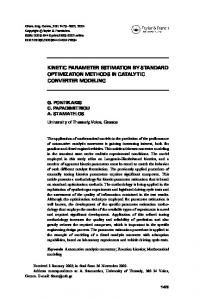
Fig. 1.7–2. Breakthrough curves for nonreactive tritium as analyzed with the two-region physical nonequilibrium model.
conductivity data. The optimized parameters were as follows: θr = 0.028, θs = 0.325, α = 0.0113 cm−1, n = 1.58, l = 0, and Ks = 19.5 cm d−1. Effluent curves derived from the laboratory miscible displacement column experiments often have been analyzed using the CFITIM (van Genuchten, 1981), CXTFIT (Parker & van Genuchten, 1984; Toride at al., 1995), and STANMOD (Šimçnek et al., 1999b) codes. These programs may be used to solve the inverse problem by fitting analytical solutions of theoretical transport models, based on the advection dispersion equation, to experimental results (see Sections 6.3 through 6.5). Figure 1.7–2 shows measured and fitted breakthrough curves of a nonreactive (3H2O) solute for transport through a Glendale clay loam soil. A tritiated water pulse of 3.102 saturated pore volumes was applied to a 30-cm-long column, with the breakthrough curve being determined from the effluent (Table 1.7–2). An analytical solution for a two-region (mobile–immobile) physical nonequilibrium model (van Genuchten, 1981) was used for the analysis (see Eq. [6.3–42] in Section 6.3). The objective function was defined as the least-squares problem β) = Φ(β
n
Σ wi[c*(ti) − c(ti,ββ)]2
i=1
[1.7–38]
with weights wi equal to one. With the pore water velocity known (v = 37.5 cm d−1) and assuming that the retardation factor R is equal to 1 for 3H2O, only three parameters were optimized against the breakthrough curve: the dispersion coefficient D (= 15.6 cm2 d−1), the dimensionless variable β (= 0.823) for partitioning mobile and immobile water in nonequilibrium transport models, and the dimensionless mass transfer coefficient ω (= 0.870). Unfortunately, the optimized parameters are highly correlated with a positive correlation for parameters D and β with the correlation coefficient RDβ = 0.96, and a negative correlation for parameters D and ω with RDω = −0.93, and β and ω with Rβω = −0.985. The high correlation between optimized parameters leads to a relatively large uncertainty of final parameter estimates, cal-
SOIL SAMPLING AND STATISTICAL PROCEDURES
153
Table 1.7–2. Measured breakthrough curve of a nonreactive solute (3H2O) for transport through a Glendale clay loam soil (fine-silty, mixed, superactive, calcareous, thermic Typic Torrifluvents). Pore volume
Concentration
Pore volume
Concentration
0.512 0.599 0.686 0.73 0.817 0.904 0.992 1.079 1.166 1.253 1.34 1.428 1.558 1.646 1.754 2.016 2.604 3.125
0.001 0.016 0.082 0.138 0.296 0.465 0.593 0.685 0.764 0.806 0.85 0.901 0.915 0.923 0.947 0.967 0.981 1
3.342 3.516 3.712 3.842 3.951 4.038 4.125 4.255 4.386 4.516 4.777 5.037 5.385 5.818 6.251 6.791 7.331 7.439
0.986 1.015 0.971 0.838 0.638 0.48 0.353 0.236 0.166 0.118 0.066 0.038 0.018 0.008 0.004 0.002 0.006 0.0003
culated using the Student’s t distribution with the 95% confidence intervals, as follows: D ∈ (7.13, 24.0 cm2 d−1), β ∈ (0.76, 0.89), and ω ∈ (0.33, 1.41). Figure 1.7–3 shows the contours of the objective function, Eq. [1.7–38], calculated at the cross-sections through the global minimum. Notice the long valleys in the horizontal direction in the D–β plane and in the vertical direction in the β–ω plane, which explains the large confidence intervals for the D and ω variables, respectively. Also notice that the contours around the minimum are only approximately elliptical. Soil hydraulic parameters are increasingly being estimated from transient variably saturated flow experiments (see Section 3.6.2). Several optimization codes have been developed that can be used only for specific applications, such as one-step (Kool et al., 1985b) or multistep outflow (van Dam et al., 1994; Chen et al., 1999) experiments. More versatile codes that can be applied to a wider range of problems with various initial and boundary conditions and several different soil layers have also been developed (Kool & Parker, 1987; Šimçnek et al., 1998, 1999a). The SFIT model (Kool & Parker, 1987) may be used to estimate soil hydraulic parameters, while the HYDRUS-1D and HYDRUS-2D models (Šimçnek et al., 1998, 1999a) can estimate simultaneously or independently both soil hydraulic and solute transport parameters from one- and two-dimensional experiments, respectively. The SFIT and HYDRUS models also consider hysteresis in the unsaturated soil hydraulic properties. In addition to codes designed specifically for estimation of soil hydraulic properties, general optimization codes, such as PEST (Doherty, 1994), LM-OPT (Clausnitzer & Hopmans, 1995), and UCODE (Poeter & Hill, 1998), can be coupled with any parameter estimation problem. Alternatively, one can also interface optimization algorithms as listed in Press et al. (1992) with specific flow and transport simulation codes. In addition, software such as MS EXCEL can now be used simply and conveniently to solve a variety of parameter estimation problems (e.g., Wraith
154
Fig. 1.7–3. Contours of the objective function (Eq. [1.7–38]) as calculated at the cross-sections through the global minimum.
CHAPTER 1
SOIL SAMPLING AND STATISTICAL PROCEDURES
155
& Or, 1998). Many examples illustrating the versatility of parameter optimization methods for estimating soil hydraulic and solute transport parameters are presented in Sections 3.6.2 and 6.6, respectively. 1.7.7 Discussion During the past two decades, curve and model fitting have become relatively standard techniques to analyze a variety of biophysicochemical data involving the unsaturated zone. Such curve fitting codes as RETC and CXTFIT are now widely used for analyzing experimental data, such as retention and conductivity data, breakthrough curves, as well as other data. A major recent promise in applying parameter estimation and nonlinear fitting techniques is the effective coupling of optimization and advanced numerical codes, and applying these codes to complex transient flow and transport experiments (see Sections 3.6.2 and 6.6). Many commonly used inversion methods (e.g., CXTFIT) are based on analytical solutions for transport or Wooding’s solution for tension infiltrometry that require relatively simple initial and boundary conditions. The resulting optimization approach then often requires experiments that repeatedly achieve steady-state or equilibrium conditions. The form of the hydraulic and transport properties is also often severely restricted using analytical methods. Application of inverse modeling techniques can alleviate some of these difficulties. Coupling of parameter estimation and nonlinear fitting techniques with numerical models provides greater flexibility by allowing different experimental boundary and initial conditions. This is important especially for field experiments where it is difficult and expensive to control the initial and boundary conditions on a large scale; parameter estimation methods permit conditions encountered in the field to be analyzed more easily. In addition, more general soil hydraulic and transport property models can be used to better represent field behavior. Analytical methods were generally preferred some 20 yr ago because of limitations in numerical methods and computer technology, thus compromising experimental procedures for the purpose of keeping the mathematics as simple as possible. Recent advances in computer software and hardware now make it possible to couple sophisticated parameter estimation algorithms with state-of-the-art, integrated numerical flow and transport codes that do not sacrifice experimental aspects for numerical expediency. The limitations of this type of parameter estimation are mostly related to factors that determine the well-posedness of the solution. For example, which variables to measure and which parameters to optimize is not known a priori for flow and transport experiments. Also, it is not obvious, in advance, whether or not a given type of experiment, or a given data set, will result in a well-posed inverse problem and how many parameters can be uniquely estimated. Since it is not always clear what is causing nonunique or unstable solutions, an inverse problem always requires in-depth analysis to determine whether it is well-posed and, if not, the cause of the ill-posedness (see also Section 3.6.2). Because of its generality (in terms of the definition of the objective function, the possible combination of boundary and initial conditions, options for considering multilayered systems, and flexibility in selecting optimized parameters), pa-
156
CHAPTER 1
rameter estimation by inverse modeling can be an extremely useful tool for analyzing a broad range of steady-state and transient, laboratory and field, flow and transport experiments. 1.7.8 References Abbaspour, K.C., M.Th. van Genuchten, R. Schulin, and E. Shläppi. 1997. A sequntial uncertainty domain inverse procedure for estimating subsurface flow and transport parameters. Water Resour. Res. 33:1879–1892. Abeele, W.V. 1984. Hydraulic testing of crushed Bandelier tuff. Report no. LA-10037-MS. Los Alamos National Laboratory, Los Alamos, NM. Akaike, H. 1974. A new look at statistical model identification. IEEE Trans. Automat. Contr., AC-19, 716–722. Akaike, H. 1977. On entropy maximization principle. p. 27–41 In P.R. Krishnaiah (ed.) Applications of statistics. North-Holland, Amsterdam, the Netherlands. Andrews, D.F., P.J. Bickel, F.R. Hampel, P.J. Huber, W.H. Rogers, and J.W. Tukey. 1972. Robust estimates of location: Survey and advances. Princeton Univ. Press, Princeton, NJ. Bard, Y. 1974. Nonlinear parameter estimation. Academic Press, New York, NY. Barhen, J., V. Protopopescu, and D. Reister. 1997. TRUST: A deterministic algorithm for global optimization. Science 276:1094–1097. Beck, J.V., and K.J. Arnold. 1977. Parameter estimation in engineering and science. John Wiley & Sons, New York, NY. Brooks, R.H., and A.T. Corey. 1966. Properties of porous media affecting fluid flow. J. Irrig. Drain. Div. Am. Soc. Civ. Eng. 92:61–88. Burdine, N.T. 1953. Relative permeability calculations from pore-size distribution data. Petrol. Trans. Am. Inst. Min. Eng. 198:71–77. Carrera, J., and S.P. Neuman. 1986a. Estimation of aquifer parameters under transient and steady state conditions. 1. Maximum likelihood method incorporating prior information. Water Resour. Res. 22:199–210. Carrera, J., and S.P. Neuman. 1986b. Estimation of aquifer parameters under transient and steady state conditions. 2. Uniqueness, stability, and solution algorithms. Water Resour. Res. 22:211–227. Chen, J., J.W. Hopmans, and M.E. Grismer. 1999. Parameter estimation of two-fluid capillary pressuresaturation and permeability functions. Adv. Water Resour. 22:479–493. Clausnitzer, V., and J. W. Hopmans. 1995. Non-linear parameter estimation: LM_OPT. General-purpose optimization code based on the Levenberg–Marquardt algorithm. Land, Air and Water Resources Paper No. 100032. University of California, Davis, CA. Doherty, J. 1994. PEST. Watermark computing. Corinda, Australia. Finsterle, S., and J. Najita. 1998. Robust estimation of hydrologic model parameters. Water Resour. Res. 34:2939–2947. Hannan, E.S. 1980. The estimation of the order of an ARMA process. Ann. Stat. 8:1971–1081. Hollenbeck, K., and K.H. Jensen. 1998. Maximum-likelihood estimation of unsaturated hydraulic parameters. J. Hydrol. 210:1992–205. Hollenbeck, K., J. Šimçnek, and M.Th. van Genuchten. 2000. RETCML: Incorporating maximum-likelihood estimation principles in the hydraulic parameter estimation code RETC. Comput. Geosci. 26:319–327. Hopmans, J.W., and J. Šimçnek. 1999. Review of inverse estimation of soil hydraulic properties. p. 643–659. In M.Th. van Genuchten et al. (ed.) Characterization and measurement of the hydraulic properties of unsaturated porous media. University of California, Riverside, CA. Huber, P.J. 1981. Robust statistics. John Wiley, New York, NY. Kashyap, R.L. 1982. Optimal choice of AR and MA parts in autoregressive moving average models. IEEE Trans. Pattern Anal. Mach. Intel. PAMI-4(2):99–104. Kool, J.B., and J.C. Parker. 1987. Estimating soil hydraulic properties from transient flow experiments: SFIT user’s guide. Electric Power Research Institute Report, Palo Alto, CA. Kool, J.B., and J.C. Parker. 1988. Analysis of the inverse problem for transient unsaturated flow. Water Resour. Res. 24:817–830. Kool, J.B., J.C. Parker, and M.Th. van Genuchten. 1985. ONESTEP: A nonlinear parameter estimation program for evaluating soil hydraulic properties from one-step outflow experiments. Bull. 853. Virginia Agric. Exp. Stn., Blacksburg, VA.
SOIL SAMPLING AND STATISTICAL PROCEDURES
157
Kool, J.B., J.C. Parker, and M.Th. van Genuchten. 1987. Parameter estimation for unsaturated flow and transport models—A review. J. Hydrol. 91:255–293. Marquardt, D.W. 1963. An algorithm for least-squares estimation of nonlinear parameters. SIAM J. Appl. Math. 11:431–441. McLaughlin, D., and L.R. Townley. 1996. A reassessment of groundwater inverse problem. Water Resour. Res. 32:1131–1161. Mualem, Y. 1976. A new model for predicting the hydraulic conductivity of unsaturated porous media. Water Resour. Res. 12:513–522. Pan, L., and L. Wu. 1998. A hybrid global optimization method for inverse estimation of hydraulic parameters: Annealing-simplex method. Water Resour. Res. 34:2261–2269. Parker, J.C., and M.Th. van Genuchten. 1984. Determining transport parameters from laboratory and field tracer experiments. Bull. 84-3. Virginia Agric. Exp. Stn., Blacksburg, VA. Poeter, E.P., and M.C. Hill. 1998. Documentation of UCODE, A computer code for universal inverse modeling. Water-Resources Investigations Report 98-4080. U.S. Geological Survey, Denver, CO. Press, W.H., B.P. Flannery, S.A. Teukolsky, W.T. Vetterling. 1992. Numerical recipes, The art of scientific computing. 2nd ed. Cambridge University Press, Cambridge, Great Britain. Russo, D., E. Bresler, U. Shani, and J. C. Parker. 1991. Analysis of infiltration events in relation to determining soil hydraulic properties by inverse problem methodology. Water Resour. Res. 27:1361–1373. Šimçnek, J., M. Šejna, and M.Th. van Genuchten. 1998. The HYDRUS-1D software package for simulating the one-dimensional movement of water, heat, and multiple solutes in variably-saturated media. Version 2.0. IGWMC-TPS-70. International Ground Water Modeling Center, Colorado School of Mines, Golden, CO. Šimçnek, J., M. Šejna, and M.Th. van Genuchten. 1999a. The HYDRUS-2D software package for simulating the two-dimensional movement of water, heat, and multiple solutes in variably-saturated media. Version 2.0. IGWMC-TPS-56. International Ground Water Modeling Center, Colorado School of Mines, Golden, CO. Šimçnek, J., M.Th. van Genuchten, M. Šejna, N. Toride, and F. J. Leij. 1999b. The STANMOD computer software for evaluating solute transport in porous media using analytical solutions of convection-dispersion equation. Versions 1.0 and 2.0. IGWMC-TPS-71. International Ground Water Modeling Center, Colorado School of Mines, Golden, CO. Toride, N., F.J. Leij, and M.Th. van Genuchten. 1995. The CXTFIT code for estimating transport parameters from laboratory or field tracer experiments. Version 2.0. Research Report no. 137. U.S. Salinity Laboratory, USDA-ARS, Riverside, CA. van Dam, J.C., J.N. M. Stricker, and P. Droogers. 1994. Inverse method to determine soil hydraulic functions from multistep outflow experiment. Soil Sci. Soc. Am. Proc. 58:647–652. van Genuchten, M.Th. 1980. A closed-form equation for predicting the hydraulic conductivity of unsaturated soils. Soil Sci. Soc. Am. J. 44:892–898. van Genuchten, M.Th. 1981. Non-equilibrium transport parameters from miscible displacement experiments. Research Report no. 119. U.S. Salinity Laboratory, USDA-ARS, Riverside, CA. van Genuchten, M.Th., F.J. Leij, and S.R. Yates. 1991. The RETC code for quantifying the hydraulic functions of unsaturated soils. EPA/600/2-91-065. USEPA, Office of Research and Development, Washington, DC. Vrugt, J.A., J.W. Hopmans, and J. Šimçnek. 2001. Calibration of a two-dimensional root water uptake model for a sprinkler-irrigated almond tree. Soil Sci. Soc. Am. J. 65:1027–1037. Wraith, J.M., and D. Or. 1998. Nonlinear parameter estimation using spreadsheet software. J. Nat. Resour. Life Sci. Educ. 27:13–19. Yeh, W.W-G. 1986. Review of parameter identification procedures in groundwater hydrology: The inverse problem. Water Resour. Res. 22:95–108.