this paper is to present a design for scenario management in Web-based ... eters including a specific combination of doctors, nurses and beds, as input.
Proceedings of the 1999 Winter Simulation Conference P. A. Farrington, H. B. Nembhard, D. T. Sturrock, and G. W. Evans, eds.
SCENARIO MANAGEMENT IN WEB-BASED SIMULATION
Andrew F. Seila
John A. Miller
Department of MIS Terry College of Business University of Georgia Athens, GA 30602-6273, U.S.A.
Department of Computer Science University of Georgia Athens, GA 30602-7404, U.S.A.
ABSTRACT
simulations, store the output data, apply appropriate methods to statistically analyze the output data (i.e., compute both parameter estimates and measures of sampling error), and present the results of the data analysis. That is, the Webbased simulation needs to include tools that let the user define and control simulation runs interactively. The purpose of this paper is to present a design for scenario management in Web-based simulation that is expected to achieve these objectives. The simulation is assumed to be correct for the intended system, so this paper does not consider problems with simulation verification. As a typical example, consider a model of a hospital emergency room. The decision maker might wish to determine appropriate staff levels (numbers of doctors and nurses) and resource levels (beds) to keep mean patient waiting times below a given maximum acceptable level. In order to do this, scenarios consisting of combinations of 1, 2, 3 and 4 doctors, 3, 4, 5, 6, 7 and 8 nurses, and all values between 11 and 20 beds are specified. The total number of scenarios is 240 in this case. For each scenario, a simulation run is defined which uses all system parameters including a specific combination of doctors, nurses and beds, as input. For each scenario, a simulation run consisting of 100 replications of 15 weeks duration is specified. The data produced by each replication consists of the mean waiting time for all patients during the last 10 weeks of the replication. The first five weeks are the warm-up period, so the waiting times produced during this period will be discarded. When the replications are run, they will be distributed among a collection of computers on the Web. Data will be collected in a database and used to compute a confidence interval for the mean waiting time for each scenario. Once the confidence intervals for all 240 scenarios are computed, the user will use a graphical tool to display them and select all scenarios for which the mean waiting time is significantly below the specified limit. Depending upon the results of this set of runs, the user might want to define further collections of scenarios and make additional runs
Internet communications in general and the World-Wide Web specifically are revolutionizing the computer industry. Today, the Web is full of important documents and clever applets. Java applets and servlets are beginning to appear that provide useful and even mission critical applications. From the perspective of simulation, a future Web will be full of simulation models and large amounts of simulationgenerated data. Many of the models will include two or three dimensional animation as well as virtual reality. Others will allow human interaction with simulation models to control or influence their execution no matter where the user is located in the world. Analysis of data from Webbased simulations involves greater degrees of freedom than traditional simulations. The number of simulation models available and the amount of simulation data are likely to be much greater. In order to assure the quality of data, the execution of models under a variety of scenarios should be well managed. Since the user community will also be larger, quality assurance should be delegated to agents responsible for defining scenarios and executing models. A major element of simulation analysis is the analysis of output data, which manages the execution of simulation models, in order to obtain statistical data of acceptable quality. Such data may be used to predict the performance of a single system, or to compare the performance of two or more alternative system designs using a single or multiple performance measures. 1
INTRODUCTION
If a Web-based simulation model is to be put to practical use to evaluate system performance and allow a decision maker to evaluate system performance and/or select from among alternative decision, then it must include software and be implemented in a way that lets the user quickly define scenarios or collections of scenarios, specify experimental designs and performance measures to be evaluated, run the
1430
Seila and Miller to refine the search for an optimal configuration for the emergency room. It might be the case that runs for some scenarios have already been made and output data are stored in a database, so these runs will not need to be executed, and the new runs can be merged with the existing runs. Additionally, the analyst could find that several designs are equivalent with respect to the mean waiting time, so she might wish to reevaluate these runs using a different performance measure or by extending the run lengths to get more precise estimates. This could require additional runs, depending upon whether appropriate data had already been collected for evaluation of the new performance measure. Thus, a scenario manager needs to provide a flexible interface with the simulation model, data sources (typically databases), and the user. It is through this interface that the user is able to implement the model as a decision support system. For the purposes of this paper, a scenario will be defined to be a single simulation run utilizing a specific set of inputs that represent a specific system configuration along with specific decisions and policies relating to the system, and produces a set of output data that can be used to compute point and interval estimates for a group of performance measures. A particular application of the model may consist of a large number of scenarios that will be searched to find the best performing decision(s). In section 2, some issues relating to input and output data are discussed. Section 3 outlines the requirements for simulation output analysis and puts them in the context of Web-based simulation. Section 4 discusses Web-based model federates. Section 5 presents a design for a scenario manager and its integration into Web-based simulation. A summary and conclusions is contained in section 6.
be noted that the collection of input data parameters defines the scenario. Thus, when defining a scenario, the input data should be linked to the scenario definition. Output data is the data produced by the simulation as it is running. Of course, these are the observations of variables measuring system behavior that are used to compute estimates of system performance measures. In real simulations, one usually records observations on many variables when the simulation is running, as opposed to just one or two variables. Thus, a simulation can produce an enormous amount of data. Even though data storage is very inexpensive, it often does not make sense to store the raw data, though this should always be kept as an option. Given all of the inputs, including the initial random number seeds, the output data can always be recreated by rerunning the simulation. This can be more or less expensive than storing the data, depending upon the complexity of the simulation. The decision about what summary statistics to store is intimately related to the experimental design and the parameters to be estimated. Normally, aggregated values or summary statistics for output data would be stored. For example, if 100 replications of a model will be run, the sample means for each variable in each replication would be stored. If the objective is to estimate the mean, this data would be sufficient, and this approach would greatly reduce the amount of storage needed. It should be noted, however, that if the objective is to estimate the 95th percentile of the distribution of the variable recorded, then the sample mean is not sufficient, and some other statistic, such as the sample 95th percentile of the observations collected in each replication would need to be stored.
2
Both input data and output data will normally be stored on a Web-enabled database, so that the simulation can access the data from any workstation on the Web that has the appropriate permission. The input data must be stored with read and write permission enabled, since the specification of a scenario would begin with a particular base set of input parameters, and then would modify some of the parameters to define the scenario. Indeed, a more efficient way of storing a scenario or group of scenarios is to reference a complete set of input parameters, then apply a "difference list" that specifies the parameters that are to be changed and the new values of these parameters. In contrast to input data, simulation output data should be stored in a read-only mode, since the only generator of this data is the simulation program. In particular, one of the security issues in a Web-based simulation is the integrity of the output data database. As mentioned earlier, each output data record must reference its associated input data to completely specify the scenario.
2.1 Data Access
WEB-BASED SIMULATION DATA
Any simulation program must deal with two types of data: input data and output data. Input data consists of all values that must be supplied to the simulation program in order for the model to be fully specified and the program to run correctly. Examples of input data for the emergency room model referred to in Section 1 are the hourly arrival rates for patients, the numbers of beds and the schedule giving the number of doctors working on each shift during the week. For a so-called trace driven simulation, the input data might also include the actual interarrival times and service times for a particular period of operation for the real system. Input data should also include all initial random number seeds so the user can have complete control over the running of the model. Since realistic simulations require large numbers of input parameters, input parameter values need to be stored in a database, and the simulation will need to be able to access the database to retrieve these values. It should also
1431
Scenario Management in Web-Based Simulation 2.2 Data Generation
protocols used to transmit the data and the security and reliability provisions for the database.
A scenario manager should be able to handle a large number of simulation runs. It could be the case that some runs have already been made and the results, i.e., output data, exist in a database. In this case, the scenario manager should be able to query the database and eliminate those runs that exist on the database. When the runs are being made, they will typically be distributed among a number of nodes on the Web. Thus, the scenario manager or some other agent will need to monitor the generation of output data and store it on the database as runs are completed.
3
There are many techniques for the analysis of simulation output. The particular technique used depends upon (1) the nature of the data produced by the model, (2) the parameter(s) to be estimated, and (3) the experimental design used in the simulation runs. This section will present a taxonomy of data analysis techniques to provide a framework for designing scenario agents, model agents and Web-based simulation systems to handle this array of possibilities. For a more in-depth discussion of simulation output analysis methods, see (Alexpoulos and Seila 1998a) or (Alexpoulos and Seila 1998b).
2.3 Data Quality Potential problems exist regarding the quality of both input data and output data. For input data, quality degradation can result from the data being old, or from the data being incomplete or having been edited and changed. The hardware and software used to store the data are assumed to be reliable. Obviously, all necessary safeguards need to be in place to prohibit the corruption of the data. To assure and maintain the quality of the data, the following facilities are recommended: • • •
SIMULATION OUTPUT DATA ANALYSIS
3.1 Finite Horizon Simulations If a simulation is designed to stop when a specified event or condition occurs, it is called a finite horizon simulation. Usually, these models represent nonstationary systems that cannot run indefinitely without becoming unstable or stopping. An example is an overloaded queueing system, where the length of the queue continues increasing indefinitely as the system runs. Data from finite horizon simulations must be collected by running independent replications, and computing one or more summary statistics from each replication. If the parameter to be estimated is the mean value of a variable, such as the mean cost before termination, then on each replication, that variable is observed and recorded. Thus, the data produced by a finite horizon simulation is a sequence of independent observations recorded from each replication. Statistical techniques appropriate for independent, identically distributed observations are used to compute point estimates and confidence intervals.
A means to automatically record dates and times the data were originally stored. A means to automatically record dates and times the data were edited. A procedure to check the input data for completeness and consistency.
The first two facilities are very similar to a revision control system, and can easily be constructed to implement a versioning system for input data. When edits are made to the data, the option can be provided to keep the older version and store the newer version of the data as a new scenario. The last item is specific to the input data. For example, if the model is a queueing system with three servers, and each server’s service time distribution has a normal distribution with its own mean and variance (truncated at zero, since service times cannot be negative), then the input data should contain three means and three variances, and the means and variances should all be positive numerical values. To handle this, the model would have to provide a set of rules for the input parameters, and the model agent would have to use these rules to determine if a particular set of input data is complete and consistent. Since the output data is generated by the simulation and cannot (or should not) be modified by any other agent, the only source of quality problems in the output data comes from transmission errors and corruption of stored data on the database. These problems are handled by the Internet
3.2 Infinite Horizon An infinite horizon simulation consists of a model of a stationary system that can conceptually run for an indefinitely long time. Examples are a stationary queueing system in which the traffic being offered to the servers is less than the servers’ capacity, and a stationary inventory system in which the inventory is periodically replenished. With infinite horizon simulations, the output data is asymptotically stationary, possibly with cyclical properties, meaning that if the simulation runs long enough, the distribution of the output data will eventually converge to a distribution that is independent of the initial state of the system when the simulation was begun. Data with these characteristics are somewhat more difficult to analyze than observations from independent replications because the analysis must identify an appropriate truncation point in the output process where
1432
Seila and Miller the influence of the initial conditions is no longer present, and the autocorrelation among the observations must be dealt with. The presence of autocorrelation means that alternative statistical techniques must be used to compute confidence intervals for the parameters to be estimated. A number of techniques are available for determining the truncation point. Unfortunately, there are none that are or can be fully automated and also are universally accepted as being reliable. As a result, it is a good idea to either use estimation techniques that are robust with respect to the truncation point, or to keep the transient data, i.e., all data from the start of the simulation runs, on the database so the user can participate in selecting the truncation point. One method that has been widely promoted is Welch’s method (Welch 1981). This method, which should be applied to a set of preliminary simulation runs, allows the user to display a graph showing how the mean of the variable of interest converges to the stationary mean. The techniques for estimating the mean of a stationary output process (with the initial transient observations removed) include batch means, independent replications, regeneration cycles, standardized time series and spectral estimation. In fact, often these techniques are used in combination. For example, batch means can be computed within independent replications or data can be batched before applying standardized time series. Techniques are also available for estimating probabilities and quantiles from stationary output processes. Computational details of these methods are available in (Alexpoulos and Seila 1998b) and the references therein. The batch means method has received a lot of attention from researchers in simulation output analysis over the past twenty-five years, and is generally accepted as being a robust and reliable method to compute confidence intervals for the mean of a stationary output process. For the batch means method, one organizes a single long simulation run into batches, computes the mean of each batch, and then applies computational methods designed for independent observations to these batch means. Theory says that if the batch size is large enough, then the batch means will be approximately uncorrelated. Fishman (Fishman 1978) proposed using an hypothesis test to determine if a set of batch means are significantly autocorrelated, and proposed a sequential procedure for increasing the batch size until there was no strong evidence of autocorrelation among batch means. (Fishman and Yarberry 1997) have developed dynamic procedures for increasing the batch size and increasing the number of batches as more data becomes available.
specified confidence interval width or statistical precision is achieved, work in an iterative manner by generation one or more observations, computing a test statistic, deciding whether to generate more data or not, and finally, computing the confidence interval. Sequential methods are easy to automate with simulations since the data are generated by a simulation program. However, they require a fundamentally different relationship between the user and the simulation model. With fixed sample size methods, all estimation computations are performed after the last simulation run. With sequential methods, some computations are done during the run and the decision to stop the run depends upon the results of these computations. Output analysis has been discussed in the context of parameter estimation and decision making. However, output analysis is also an integral part of the system validation process, in which data from the simulation is compared to data from the real system and a conclusion is drawn as to whether the model is an adequate representation of the real system. In this case, output data must be collected and analyzed, but also the analyst must have access to a database of data from the real system. This data is not input data, but measurements on “output variables,” i.e., variables that measure system performance, such as waiting times or queue lengths. 3.4 Multivariate Methods and Graphical Presentations Output analysis generally doesn’t stop with confidence intervals for a single parameter. Usually, multiple parameters are estimated and simultaneous confidence intervals are computed. Simultaneous confidence intervals are a set of confidence intervals which include all parameters with a given probability. A number of multivariate techniques are available for computing simultaneous confidence intervals. Analysts also have the need to examine relationships between variables in simulations by fitting statistical models to the output data. Such a model is often called a metamodel. These models frequently take the form of regression models where one performance measure is expressed as a linear or nonlinear function of input parameters. Graphical displays are an indispensable part of output analysis, both for summarizing the results of single and multiple scenarios, and for examining the characteristics within individual simulation runs or scenarios. For example, to display the results of multiple scenarios, one might use a graph to show the relationship between mean patient waiting time and the number of doctors on duty in an emergency room. Or, within a single simulation run, one might display the p-values of von Neumann’s test for serial correlation to judge how well the batch size was chosen. Given the requirements of the output analysis methods and adding the environment of Web-based simulation, it seems clear that the design of a system to provide output
3.3 Sequential Methods Sequential methods are available for estimating parameters. These methods, which aim to generate data until a pre-
1433
Scenario Management in Web-Based Simulation jqds
analysis is challenging. The simulation runs can be done on multiple nodes, so data must be collected and coordinated from multiple locations. The actual simulation model could be obtained on the Web, so the user may not be familiar with the details of the model. Users of the output analysis can also be distributed, so the application of output analysis methods and the display of results also must be coordinated. 4
QDS Agent
EXECUTE
STORE
VIEW
jmodel
jrun
jquery
jview
Synthesis Agent
Scenario Agent
DBQuery Agent
Analysis Agent
Design Agent
Model Agent
DBUpdate Agent
Browsing Agent
MODEL FEDERATES
Since the simulation will be Web-based, a model can actually consist of a collection of models distributed on the Web. For example, consider once again the emergency room model. It could consist of a model representing arrivals to the emergency room from various sources, a model of emergency room operations, and models of lab operations and x-ray department services. These models could be stored on different nodes on the Web, but collected and run on a single computer, or the runs themselves could be distributed. Models can communicate with one another using standard Web protocols. Normally, one would expect the relationships and dependencies between model components to be loose because communication over the Web is currently much slower than communication within a single node. Thus, simulation runs would be unacceptably slow if communication between nodes is a significant part of the model run. The model includes the actual simulation code, but it also must include an interface to access and input the model parameters, and specify what variables are to be observed and recorded during the simulation run. This object is supplied to the scenario agent by the model agent so the user can specify the input parameters for a specific run or set of runs. This interface should also provide any other model specifics that might be used in output analysis. For example, if the model has a natural cycle of a week, then the model should be run for a number of weeks and the data should be collected in units of weeks. 5
DESIGN
Databases
Bank
FoodCourt
ERoom
Model Repositories
Figure 1: JSIM Schematic Diagram
Agent Design Synthesis Model Scenario DBUpdate DBQuery Browsing Analysis QDS
Table 1: JSIM’s Agents Expertise Visually designing simulation models. Composing model federations. Managing model execution. Running federations under scenarios. Updating databases. Querying databases. Browsing databases and repositories. Analyzing/visualizing results. Automating simulation and modeling.
low. Since this paper is focused on generating, analyzing and viewing simulation data, only the jrun and jview packages will be discussed in detail (see Miller et al. 1999) for a discussion of other packages).
PROVIDING AND CONTROLLING DATA THROUGH AGENTS
5.1 Design Agents
The JSIM project (Nair et al. 1996; Miller et al. 1997; Miller et al. 1998; Miller et al. 1999) includes output analysis as part of a Web-based simulation modeling system. The system in general consists simulation models implemented as Java Beans and executed within an environment consisting of specialized agents. Each of the agents are also implemented as Java Beans. Figure 1 shows a schematic depicting the relationship between these components (beans). The function and purpose of each type of agent is defined in Table 1. Each of the five agent packages (jmodel, jrun, jquery, jview and jqds) is briefly discussed in the subsections be-
1434
The jmodel package contains agents (beans) for designing and synthesizing models and model federations. Theses agents facilitate rapid visual design of simulation models. Since these agents are only concerned with developing and verifying models, and not with actually executing the models in production runs, they do not need to communicate with any agents other than the QDS agent. 5.2 Execution Agents The other agents in Figure 1 are concerned with creating scenarios, running the simulations, storing the results and
Seila and Miller analyzing the data produced. That is, the rest of the agents are concerned with utilizing the simulation as a decision support system. The jrun package contains agents (beans) to control the execution of models and model federations.
scenarios exist in a database and if not, provide a list of scenarios that do exist. It can also manage the collection and storage of output data for a scenario or collection of scenarios. If output data are to be accessed and analyzed by the output analysis agent, the database agent can query the database and either provide the user with the requested data or report that it cannot be found and provide a list of scenarios that are present on the database.
5.2.1 Model Agents A model agent provides the interface between the model and all other agents in the system. Thus, the model must only be concerned with communication with the model agent, and the model agent then can provide the necessary information to the other agents. For example, the model agent can get the input parameter dialog from the model, and pass it on to the scenario agent so it can be displayed and input data provided by the user. The model agent manages and monitors the execution of the model and is responsible for stopping the model. It can also query the model about the types of output analysis that are appropriate for the output data, and can provide this information to the user. Thus, if the model is not stationary, only independent replications can be run and it does not make sense to specify that output be batched. Output data is transmitted to the model agent, who then passes it to the database agent to be stored on the database. It is also the model agent’s responsibility to associate a particular set of input data with the output data to fully specify the scenario to the database agent.
5.4 View Agents The jview package contains agents (beans) for conveniently accessing and visualizing simulation data as well as simulation models. These agents work naturally together because a user might want to search for models of particular systems and, if the models are found, she might want to examine the results of some scenarios that have been run. 5.4.1 Browsing Agents These agents make it easy for users or other agents to access information in simulation databases or model repositories. They are ideal when one is looking for available simulation results or possible models to run. 5.4.2 Analysis Agents
5.2.2 Scenario Agents
An analysis agent performs statistical computations for detailed output analysis and provides the results in text and graphical form. A model agent will store intermediate results (e.g., all batch means and variances for all monitored variables) in a database for post-processing by an analysis agent. To a large extent, this agent is much like a statistical analysis program. It must be able to handle much of the requirements for estimation of the mean and quantiles for i.i.d. data, and in addition it needs to implement some of the methods for estimation of the mean and quantiles for stationary data. It is necessary that the results of output analysis be presented in graphical form so they can be displayed locally and over the Web. Thus, the analysis agent must be able to produce various graphs, especially histograms, bar charts, line graphs, scatterplots, and versions of these with error bars. Additionally, an analysis agent may be used on data sets used to determine inputs to simulations. The statistical methods normally applied to input data involves estimating parameters of candidate distributions and testing for goodness of fit for these distributions. Other methods needed for input data analysis include fitting of statistical models and analysis of time series data. Since these techniques overlap considerably with those needed for output analysis, it makes sense to include these in the analysis agent.
A scenario agent provides a high-level graphical user interface (GUI) allowing a user to define a scenario under which to run a model or model federation. Thus, the scenario agent allows the user to (1) specify a collection of input parameters to define a scenario, (2) specify a collection of variables on which to collect observations, (3) provide the experimental design, i.e., how many replications to run, how many batches per replication, etc., (4) provide additional scenario identification such as a descriptive phrase for the scenario, and (5) present any other objects that are provided by the model through the model agent. An example of the last item is an animation that the model might provide while the simulation is running, although normally animations are not made on production runs. The scenario agent must interface with the database agent to store the input parameters and descriptive data for each scenario. 5.3 Storage Agents The jquery package contains agents (beans) that make it easy for other agents to access a variety of databases. The database agents (DBUpdate and DBQuery) facilitate communication between the model agent, scenario agents, output analysis agents and the databases. Such an agent can query the database of simulation results to see if any specified
1435
Scenario Management in Web-Based Simulation Miller, J., Ge, Y., and Tao, Z. (1998). Component-Based Simulation Environments: JSIM as a Case Study Using Java Beans. In Proceedings of the 1998 Winter Simulation Conference, pages 786–793, Washington, DC. Miller, J., Nair, R., Zhang, Z., and Zhao, H. (1997). JSIM: A Java-Based Simulation and Animation Environment. In Proceedings of the 30th Annual Simulation Symposium, pages 31–42, Atlanta, Georgia. Miller, J., Seila, A., and Xiang, X. (1999). The JSIM WebBased Simulation Environment. Future Generation Computer Systems. Miller, J. and Weyrich, O. (1989). Query Driven Simulation Using SIMODULA. In Proceedings of the 22nd Annual Simulation Symposium, pages 167–181, Tampa, Florida. Nair, R., Miller, J., and Zhang, Z. (1996). A Java-Based Query Driven Simulation Environment. In Proceedings of the 1996 Winter Simulation Conference, pages 786– 793, Coronado, California. Welch, P. D. (1981). On the problem of the initial transient in steady state simulations. Technical Report, IBM Watson Research Center, Yorktown Heights, NY.
5.5 QDS Agent A user may interact with with any of the following three packages jmodel, jrun or jview in order to design, execute and view the results of simulation models. A QDS agent is an attempt to build an intelligent agent to automate and make transparent the steps necessary to produce simulation results. Users ask questions and the agent responds to the users query; hence the name Query Driven Simulation (QDS) (Miller and Weyrich 1989). For more details about this agent see (Miller et al. 1999). 6
CONCLUSIONS AND FUTURE WORK
The objective of the JSIM project is to provide a flexible, platform-independent, user-friendly environment for developing and running simulation models on the Web. This paper has outlined the needs of the end-user who plans to use the Web-based simulation models as a decision analysis tool. The requirements for scenario development and output analysis have been outlined and a design for the environment that includes these requirements has been provided. The JSIM project is currently implementing this design. JSIM is open source software that is freely available on the Web and can be modified by anyone.
AUTHOR BIOGRAPHIES ANDREW F. SEILA is an Associate Professor in the Terry College of Business at the University of Georgia, Athens, Georgia. He received his B.S. in Physics and Ph.D. in Operations Research and Systems Analysis, both from the University of North Carolina at Chapel Hill. Prior to joining the faculty of the University of Georgia, he was a Member of Technical Staff at the Bell Laboratories in Holmdel, New Jersey. His research interests include all areas of simulation modeling and analysis, especially output analysis. He has been actively involved in the Winter Simulation Conference since 1977, and served as Program Chair for the 1994 conference.
http://orion.cs.uga.edu:5080/∼jam/jsim The authors invite anyone who is interested in participating to contact them. Currently, prototype versions of jmodel, jquery, and jrun are available. Work is ongoing on jview and jqds. REFERENCES Alexopoulos, C. and Seila, A. (1998) Output Data Analysis. Chapter 7 inHandbook of Simulation, John Wiley and Sons, pages 225–272, New York. Alexopoulos, C. and Seila, A. (1998) Advanced Methods for Simulation Output Analysis. In Proceedings of the 1998 Winter Simulation Conference, pages 113–120, Washington, DC. Fishman, G. S. (1998). Labatch.2: Software for statistical analysis of simulation sample path data. In Proceedings of the 1998 Winter Simulation Conference, pages 131– 139, Washington, DC. Fishman, G. S. (1996). Monte Carlo: Concepts, Algorithms and Applications. John Wiley and Sons, New York Fishman, G. S. (1978) Grouping observations in digital simulation. Management Science, Vol. 24, pages 510–521. Fishman, G. S. and Yarberry, S. (1997) An implementation of the batch means method. INFORMS Journal on Computing, Vol. 9, pages 296–310.
JOHN A. MILLER is an Associate Professor and the Graduate Coordinator in the Department of Computer Science at the University of Georgia. His research interests include Database Systems, Simulation and Workflow as well as Parallel and Distributed Systems. Dr. Miller received the BS degree in Applied Mathematics from Northwestern University in 1980, and the M.S. and Ph.D. in Information and Computer Science from the Georgia Institute of Technology in 1982 and 1986, respectively. During his undergraduate education, he worked as a programmer at the Princeton Plasma Physics Laboratory. Dr. Miller is the author of over 60 technical papers in the areas of Database, Simulation and Workflow. He has been active in the organizational structures of research conferences in all these three areas. He has served in positions from Track Coordinator to Publications Chair to General Chair of the following conferences:
1436
Seila and Miller Annual Simulation Symposium (ANSS), Winter Simulation Conference (WSC), Workshop on Research Issues in Data Engineering (RIDE), NSF Workshop on Workflow and Process Automation in Information Systems, and Conference on Industrial & Engineering Applications of Artificial Intelligence and Expert Systems (IEA/AIE). He has also been a Guest Editor for the International Journal in Computer Simulation as well as IEEE Potentials.
1437