This algorithm is a reformulation of the well-known AC3 al- gorithm. The evaluation section shows that 2-C3 is able to prune more search space than AC3 and ...
2-C3: From Arc-Consistency to 2-Consistency Marlene Arangu´ and Miguel A. Salido and Federico Barber Instituto de Autom´atica e Inform´atica Industrial Universidad Polit´ecnica de Valencia. Valencia, Spain
Abstract Arc consistency algorithms are widely used to prune the search space of Constraint Satisfaction Problems (CSPs). Since many researchers associate arc consistency with binary normalized CSPs, there is a confusion between the notion of arc consistency and 2-consistency. 2-consistency guarantees that any instantiation of a value to a variable can be consistently extended to any second variable. Thus, 2-consistency can be stronger than arc-consistency in binary CSPs. In this paper, we present a new algorithm, called 2-C3, wich achieves 2-consistency in binary and non-normalized CPSs. This algorithm is a reformulation of the well-known AC3 algorithm. The evaluation section shows that 2-C3 is able to prune more search space than AC3 and AC4.
Introduction Constraint programming is a software technology for the description and effective solving of large and complex problems ( in many areas of the real life), particularly combinatorial problems (Dechter 2003; Bart´ak 1999). Many of these problems can be modeled as constraint satisfaction problems (CSPs) and can be solved using constraint programming techniques. The basic idea of CSP is to model the problem as a set of variables with finite domains (the values for the variables) and a set of constraints that impose a limitation on the values that a variable, or a combination of variables, may be assigned. The task is to find an assignment of values for the variables that satisfy all the constraints. In general, the tasks posed in the CSP paradigm are computationally intractable (NP-Complete). Some of the algorithms used to manage CSP are systematic search, constraint propagation and consistency techniques. For reasons of brevity in this paper we only explain the consistency techniques. The consistency-enforcing algorithm performs any partial solution of a small sub-network that is extensible to a surrounding network. The number of possible combinations can be huge, while only very few are consistent. By eliminating redundant values from the problem definition, the size of the solution space decreases. If any domain becomes empty as a result of reduction, then it is immediately known that the problem has no solution (Ruttkay 1998). There exist c 2009, Association for the Advancement of Artificial Copyright ° Intelligence (www.aaai.org). All rights reserved.
many levels of consistency depending on the number of variables involved: node-consistency involves only one variable; arc-consistency involves two variables; path-consistency involves three variables; and k-consistency involves k variables. More information can be seen in (Bart´ak 2001; Dechter 2003). Arc-consistency algorithms are a major component of many industrial and academic CSP solvers. Arc consistency algorithms are based on the notion of support. These algorithms ensure that each value in the domain of each variable is supported by one o more values in the domain of each variable by which it is constrained. Arc consistency algorithms which lie at the heart of a CSP solver, are very-time consuming. For this reason, arc consistency algorithms and their time complexity are areas that have been heavily researched (van Dongen, Dieker, and Sapozhnikov 2008). Proposing efficient algorithms to enforce arc-consistency has always been considered as a central question in the constraint reasoning community. Thus, there are many arc-consistency algorithms such as: AC1, AC2, and AC3 (Mackworth 1977); AC4 (Mohr and Henderson 1986); AC5 (Perlin 1992; Hentenryck, Deville, and Teng 1992); AC6 (Bessiere and Cordier 1993); AC7 (Bessiere, Freuder, and R´egin 1999); AC8 (Chmeiss and Jegou 1998); AC2001, AC3.1 (Bessiere et al. 2005); and more. However, AC3 and AC4 are the ones most often used (Bart´ak 2001). Algorithms that perform arc-consistency have focused their improvements on time-complexity and spacecomplexity. The main improvements have been achieved by: changing the means of propagation from arcs to values, (i.e., changing the granularity from coarse-grained to finegrained); appending new structures; performing bidirectional searches (AC7); changing the support search: searching for all supports (AC4) or searching for only the necessary supports (AC6, AC7, AC8 and AC2001); improving the propagation (i.e., AC7 and AC2001, which perform propagation only when necessary); etc. The concept of consistency was generalized to kconsistency by (Freuder 1978). Thus, 2-consistency is related to constraints that involve two variables. Furthermore, many works on arc-consistency made the simplified assumptions that CSPs are binary (all constraints involve two variables) and normalized (two different constraints do not involve exactly the same variables), these notations are very
simple and the new concepts are easy to present. In their work (Rossi, Van Beek, and Walsh 2006) show a strange effect of associating arc-consistency with binary normalized CSPs: the confusion between the notions of arc-consistency and 2-consistency (2-consistency guarantees that any instantiation of a value to a variable can be consistently extended to any second variable). In binary CSPs, 2-consistency is at least as strong as arc-consistency. When the CSP is binary and normalized, arc-consistency and 2-consistency perform the same pruning. However, this is not true in general. For more details see (Rossi, Van Beek, and Walsh 2006). Few works have been done to develop algorithms to achieve 2-consistency in binary CSPs. Therefore, in the following section, we provide the necessary definitions to understand the rest of the paper, and we present an example to clarify some important concepts. Later, we present our 2C3 algorithm. This algorithm is a reformulation of AC3 to achieve 2-consistency in binary and non-normalized CSPs. An evaluation is presented to compare the behavior of the 2-C3 algorithm against AC3 and AC4 algorithm. Finally, some conclusions are presented.
Definitions By following the standard notations and definitions in the literature (Bessiere 2006; Bart´ak 2001; Dechter 2003), we have summarized the basic definitions that are used throughout the paper. Definition 1. Constraint Satisfaction Problem (CSP) is a triple P = hX, D, Ri where: X is the finite set of variables {X1 , X2 , ..., Xn }; D is a set of domains D = D1 , D2 , ..., Dn such that for each variable Xi ∈ X there is a finite set of values that the variable can take; R is a finite set of constraints R = {R1 , R2 , ..., Rm } which restrict the values that the variables can take simultaneously. Definition 2. Binary constraint. A constraint is binary if it involves only two variables. A CSP is binary iff all constraints are binary. Definition 3. Block of constraints. A block of constraints Cij is a set of binary constraints that involve the same variables Xi and Xj . Definition 4. Normalized CSP. A CSP is normalized iff two different constraints do not involve exactly the same variables. Definition 5. Instantiation. It is a pair hXi , ai, which represents an assignment of the value a to the variable Xi , and a is in the domain of Xi . We can use (Xi = a) ≡ hXi , ai. Definition 6. Constraint Satisfy: A constraint Rij is satisfied if the instantiation of hXi , ai and hXj , bi is legal for this constraint (hXi , ai, hXj , bi) ∈ Rij . Definition 7. Value arc-consistency. A value a ∈ Di is arc-consistent relative to Xj , iff there exists a value b ∈ Dj such that (Xi , a) and (Xj , b) satisfy the constraint Rij ((Xi = a, Xj = b) ∈ Rij ). Definition 8. Variable arc-consistency: A variable Xi is arc-consistent relative to Xj iff all values in Di are arcconsistent. Definition 9. CSP arc-consistency. A CSP is arcconsistent iff all the variables are arc-consistent, e.g., all the
constraints Rij and Rji are arc-consistent. (Note: here we are talking about full arc-consistency). Definition 10. Value 2-consistency. A value a ∈ Di is 2-consistent relative to Xj , iff there exists a value b ∈ Dj k such that (Xi , a) and (Xj , b) satisfy all the constraints Rij k (∀k : (Xi = a, Xj = b) ∈ Rij ). Definition 11. Variable 2-consistency: A variable Xi is 2-consistent relative to Xj iff all values in Di are 2consistent. Definition 12. CSP 2-consistency. A CSP is 2-consistent iff all the variables are 2-consistent, e.g., any instantiation of a value to a variable can be consistently extended to any second variable. We will focus our attention on binary and non-normalized CSPs. Figure 1 left shows a binary CSP, which is presented in (Rossi, Van Beek, and Walsh 2006) with two variables X1 and X2 , D1 = D2 = {1, 2, 3} and two constraints 0 R12 : X1 ≤ X2 , R12 : X1 6= X2 . It can be observed that this CSP is arc-consistent due to the fact that every value of every variable has a support for constraints R12 0 and R12 . In this case, arc-consistency does not prune any value of the domain of variables X1 and X2 . However, as (Rossi, Van Beek, and Walsh 2006) show, this CSP is not 2-consistent because the instantiation X1 = 3 can not be extended to X2 and the instantiation X2 = 1 can not be extended to X1 . Thus, Figure 1 right presents the resultant CSP filtered by arc-consistency and 2-consistency. It can be observed that 2-consistency is at least as strong as arcconsistency.
The Cost of Translating a non-normalized CSP into a Normalized One The only way to translate a non-normalized CSP into a normalized one is by means of the extensional representation of constraints. It is well known that a constraint can be represented intensionally (by an expression) or extensionally (by the set of allowed or disallowed tuples). The vast majority of constraints presented in real problems are modeled intensionally. Some of these constraints are then extensionally represented to be managed by CSP solvers, filtering techniques, etc. However, this is a very hard task, particulary if the domains are huge or impossible in continuous domains. Actually, from the mathematical point of view, the extensional and intensional representation are equal. From the computation perspective, however, the intensional one is a lot more compact and expressive than the extensional one. For instance, for D1 = D2 = {0, 1, 2}, a constraint C12 with the intensional meaning R12 : X1 < X2 could be defined extensionally by allowed tuples R12 = {(0, 1), (0, 2), (1, 2)} or disallowed tuples R12 = {(0, 0), (1, 0), (1, 1), (2, 0), (2, 1), (2, 2)}. In CSPs with large domains, for instance, D1 = D2 = {1, 2, ..., 1000}, a constraint C12 with the extensional representation generates one million of tuples (D1 xD2 ) to be labeled as allowed or disallowed tuples. This task has a high temporal and spatial complexity. Once, all the constraints of the non-normalized CSP have been translated into an extensional representation (allowed
Figure 1: Example of Binary CSP. or disallowed tuple sets), the constraints that involve the same variables must be grouped in order to select all intersected tuples. For instance, if there exist two constraints that 0 0 involve variable i and j (Rij , Rij ), and Sij , Sij are the sets of allowed tuples respectively, then Cij = {(a, b)|(a, b) ∈ 0 Sij ∧ (a, b) ∈ Sij } For instance, Figure 2 shows an example of nonnormalized CSP due to the fact that variables X1 and X2 0 ). are restricted by two different constraints (R12 and R12 The Cartesian Product of variable domains is D1 xD2 = {(0, 0), (0, 1), (0, 2), (1, 0), (1, 1), (1, 2), (2, 0), (2, 1), (2, 2)}. The allowed tuples for the constraint R12 are S12 = {(0, 0, (0, 1), (0, 2), (1, 1), (1, 2), (2, 2)}, 0 are while the allowed tuples for the constraint R12 0 S12 = {(0, 1), (0, 2), (1, 0), (1, 2), (2, 0), (2, 1)}; so that 0 = {(0, 1), (0, 2), (1, 2)}. Thus, by apC12 = S12 ∩ S12 plying arc-consistency we can achieve the reduced domains D1 = {0, 1} and D2 = {1, 2}. Although this translation technique is quite simple, its implementation consumes a lot of time and requires the generation of structures that consume memory. In conclusion, the cost of translating a non-normalized CSP into a normalized one is a prohibitive task in problems with large domains. The main research carried out regarding filtering techniques for constraint satisfaction has focused attention on normalized CSPs or extensionally represented constraints. However, real life problems are usually represented as CSPs with non-normalized CSPs with intensionally represented constraints. Therefore, the development of filtering techniques to manage these problems is necessary.
Algorithm 2-C3 2-consistency guarantees that any instantiation of a value to a variable can be consistently extended to any second variable. While arc-consistency only checks the support hold in the constraint, 2-consistency checks the support hold in all constraints of the set. Therefore, 2-consistency can be stronger than arc-consistency in binary CSPs. Following, we present a new algorithm called 2-C3 that
achieves 2-consistency in binary and non-normalized CSPs. This algorithm is a reformulation of the well-known AC3 algorithm. The main algorithm is a simple loop (see Algorithm 2, lines 10-20) that selects and revises the block of constraints stored in a queue Q (see Algorithm 1) until no change occurs (Q is empty), or until the domain of a variable becomes empty. The first case ensures that all values of domains are consistent with all constraints, and the second case returns that the problem has no solution. Algorithm 1 Revise procedure Input: A CSP P 0 defined by two variables X = (Xi , Xj ), domains Di and Dj , and constraint set Cij . Output: Di , such that Xi is 2-consistent relative Xj and the boolean variable change 1: change ← false 2: for each a ∈ Di do 3: if @b ∈ Dj such that (Xi = a, Xj = b) ∈ Cij then 4: remove a from Di 5: change ← true 6: end if 7: end for 8: return change The Revise procedure of 2-C3 is very close to the Revise procedure of AC3. The only difference is that the instantiation (Xi = a, Xj = b) must be checked with the block of constraints Cij instead of with only one constraint. This set of constraints Cij could also be ordered in order to avoid unnecessary checks. If we order this set from the tightest constraint to the loosest constraint, the constraint checking will find inconsistency constraints sooner, in which case no further constraint checks must be carried out. For the example shown in Figure 2, Q initially stores 0 0 the constraints Q = {C02 , C20 , C12 , C21 }. This table also shows the corresponding constraints (Figure 2, right). Table 1 shows how the 2-C3 procedure evaluates each constraint for this example. In loops 1 and 2, sets C02 and 0 0 C02 have only one constraint: R02 and R02 ,respectively.
Figure 2: Example of Binary non-normalized CSP. The arc-consistency algorithms do not perform any pruning, unless normalization is performed on the restrictions. Algorithm 2 2-C3 procedure Input: A CSP, P = hX, D, Ri Output: true and P 0 (which is 2-consistent) or false and P 0 (which is 2-inconsistent because some domain remains empty) 1: for every i, j do 2: Cij = ∅ 3: end for 4: for every arc Rij ∈ R do 5: Cij ← Cij ∪ Rij 6: end for 7: for every set Cij do 8: Q ← Q ∪ {Cij , Cji } 9: end for 10: while Q 6= ∅ do 11: select and delete Cij from queue Q 12: if Revise(Cij ) = true then 13: if Di 6= ∅ then 14: Q ← Q ∪ {(Cki | k 6= i, k 6= j} 15: else 16: return false /*empty domain*/ 17: end if 18: end if 19: end while 20: return true
AC3 and AC4 do not prune any value nor do they carry out any propagation. AC3 carries out 29 constraint checkings, and AC4 carries out 54 constraint checkings. Table 1: Loops carried out by 2-C3 for the example shown in Figure 2. Loop
Set Cij
1
C02
1 2 0 2
0 C20
1 2
val b 0 0 1 0 1 2 0 0 1 0 1 2 0
0 1 0 3
C12
1
1 2
2
0 1 2
0 4
Thus, their checks are equivalent to AC3, however, in loops 3 and 4, each set has two constraints, so 2-C3 checks that both values hold with all the constraints of the set. Thus, in loop 3, where C12 is processed, it is verified whether or not value 0 of D1 has support with value 0 of D2 . This is true for R12 ; however, when the same values are checked 0 with the next constraint of set (R12 ), this constraint is not satisfied. For this reason, the next value in D2 (value 1) is 0 sought, and both constraints (R12 , R12 ) are satisfied with values X1 = 0 and X2 = 1. We denote the set that must be re-evaluated (C02 ) using dotted lines. This set constraint was added to the queue Q (See Table 1, loop 4). In the above example to achieve 2-consistency, 2-C3 performs 3 prunes of domain values, carries out 37 constraint checkings (Cc), and carries out 1 propagation (Np) in Q.
val a 0
0 C21
1 1 2 0
5
C02
0
1 2
0 0 1 2 1 1 2
Rij R02 R02 R02 R02 R02 R02 0 R20 0 R20 0 R20 0 R20 0 R20 0 R20 R12 R120 R12 R120 R12 R12 R120 R12 R120 R12 R12 R12 R120 0 R21 0 R21 0 0 R21 0 R21 0 R21 0 0 R21 0 R210
hold yes no yes no no yes yes no yes no no yes yes no yes yes no yes no yes yes no no yes no yes no no yes yes yes yes
R02 R02 R02 R02 R02
no no yes no yes
change
Prune Xi
Add Q
false
false
true
hX1 , 2i
true
hX2 , 0i
C02 true
hX2 , 0i
Experimental Results In this section, we compare the behavior of the arcconsistency algorithms AC3 and AC4 and our proposed 2-consistency algorithm (2-C3). Furthermore, we implemented the most efficient versions of AC3 and AC4 with the improvement shown in (Mackworth 1977; Dechter 2003; Bessiere 2006; Bart´ak 2001), in order to remove ambiguity and improving efficiency.
Table 2: Number of pruning and constraint checks by using AC3, AC4 and 2-C3 in problems < n, 20, 800, 2 >. value n 50 70 90 110 130 150
Arc-consistency AC AC3 AC4 pruning checks checks 331 351565 642314 303 339410 660984 289 324385 671040 240 317697 681837 255 295527 682225 254 267646 684949
2-consistency 2-C3 pruning checks 627 496202 582 546119 566 512247 559 475114 554 462976 548 411415
The experiments were performed on random instances. A random CSP instance was characterized by the 4-tuple < n, d, m, c >, where n was the number of variables, d the domain size, m the total number of binary constraints and c the number of constraints in each block. The constraints were in the form Xi op Xj , where Xi , Xj ∈ X and op ∈ {, ≥}. We randomly generated binary and non-normalized problems. All the variables maintained the same domain size. The problems were randomly generated by modifying these parameters. We evaluated 50 test cases for each type of problem. Thus, Tables 2 and 3 fixed three of the parameters and varied the other one in order to evaluate the algorithm performance when this parameter was increased. Performance was measured in terms of number of values pruned. All algorithms were written in C. The experiments were conducted on a PC Pentium IV (3.0 GHz processor and 1 GB RAM). Table 2 shows the number of constraint checks and prunes using AC3, AC4 and 2-C3: the number of variables was increased from 50 to 150; the domain size was set to 20; the number of constraints was set to 800; and the number of blocks of constraints was set to 2 ( < n, 20, 800, 2 >). The results show that the number of prunes was lower in both AC3 and AC4 than in 2-C3 in all cases. This is due to the fact that the problems start with same domain size (from 1 to 20) and they have constraints with operators (=, 6=, ≤, or ≥). Therefore, AC3 and AC4 did not prune any value by analyzing the constraints individually. However, 2-C3 analyzed the blocks of constraints that had a mix of these operators, and it was able to prune more search space. Furthermore, the ratio between checks and prunes of 2C3 was better than both AC3 and AC4 (845 checks/pruning for 2-C3; 1141 checks/pruning for AC3; and 2403 checks/pruning for AC4). Thus, the large number of checks for 2-C3 was offset by a greater amount of pruning. Table 2 also shows that the number of constraint checks and pruned values was reduced since the number of variables increased in AC3, AC4, and 2-C3. Arc-consistency is reached sooner because the number of variables increased and the number of constraints remained constant. Thus, the random problems were loose. Table 3 presents the number of constraint checks, where the number of constraints was increased from 50 to 700 and the number of variables, the domain size, and block of constraints were set at 50, 20, and 2, respectively (
Table 3: Number of pruning and constraint checks by using AC3, AC4 and 2-C3 in problems < 50, 20, m, 2 >. value m 50 100 150 200 300 450 600 700
Arc-consistency AC AC3 AC4 pruning checks checks 17 11559 43449 34 25245 86475 53 46410 130053 61 56745 172084 104 111268 255652 172 178341 376226 218 240995 496307 285 297126 567492
2-consistency 2-C3 pruning checks 34 13455 70 37422 106 65060 140 99430 217 166531 330 283190 447 396326 535 451253
< 50, 20, m, 2 >). As in the above evaluation, the results were similar. 2-C3 was able to carry out more pruning (> 50%) than AC3 and AC4. In this case, the number of constraint checks increased as the number of constraints increased. Since the random problems maintained the same number of variables but the number of constraints increased, the random problems were tight.
Table 4: Number of pruning and constraint checks by using AC3, AC4 and 2-C3 in inconsistent problems < n, 20, 1200, 2 >. value n 50 70 90 110 130 150
Arc-consistency AC3 AC4 pruning checks pruning checks 1447 1896 2396 712 927 1170
143166 150560 169577 180873 217657 237029
712 927 1146 1429 1638 1665
728983 748371 796207 817588 856362 865837
2-consistency 2-C3 pruning checks 1179 1763 1083 642 716 1063
166639 125626 134138 142184 170743 115141
Table 5: Number of pruning and constraint checks by using AC3, AC4 and 2-C3 in inconsistent problems < 50, 20, m, 2 >. value m 150 300 450 600 750 900 1050 1200
Arc-consistency AC3 AC4 pruning checks pruning checks 863 904 881 893 712 711 697 719
104619 85368 90910 98802 100136 114720 129463 142499
323 611 722 708 709 711 697 719
119852 224419 321714 410981 482775 566505 649768 728237
2-consistency 2-C3 pruning checks 605 647 485 521 463 669 563 556
29756 44464 48963 69526 83646 115648 131904 141429
Tables 4 and 5 show the number of constraint checkings and propagations in inconsistent instances where the number of variables (n) or the number of constraints increased (m), respectively. 2-C3 carried out fewer prunes and fewer checkings than AC3 and AC4, 2-C3 was more efficient in detecting inconsistencies.
Conclusions Filtering techniques are widely used to prune the search space of CSPs. AC3 is one of the best known arc consistency algorithms, and different versions have improved the efficiency of the original one. Since many researchers associate arc consistency with binary normalized CSPs, there is a confusion between the notion of arc consistency and 2consistency. In this paper, we have presented a reformulation of AC3 to achieve 2-consistency in binary and nonnormalized CPSs. The evaluation section shows that 2-C3 achieves 2-consistency and is therefore able to prune more search space than both AC3 and AC4. This filtering algorithm could be very appropriate in search tools to manage non-normalized problems.
References Bart´ak, R. 1999. Constraint programming: In pursuit of the holy grail. In MatFyzPress., ed., Proceedings of the Week of Doctoral Students (WDS99), Part IV. Bart´ak, R. 2001. Theory and practice of constraint propagation. In Figwer, J., ed., Proceedings of the 3rd Workshop on Constraint Programming in Decision and Control. Bessiere, C., and Cordier, M. 1993. Arc-consistency and arc-consistency again. In Proc. of the AAAI’93, 108–113. Bessiere, C.; R´egin, J. C.; Yap, R.; and Zhang, Y. 2005. An optimal coarse-grained arc-consistency algorithm. Artificial Intelligence 165:165–185. Bessiere, C.; Freuder, E.; and R´egin, J. C. 1999. Using constraint metaknowledge to reduce arc consistency computation. Artificial Intelligence 107:125–148. Bessiere, C. 2006. Constraint propagation. Technical report, CNRS/University of Montpellier. Chmeiss, A., and Jegou, P. 1998. Efficient pathconsistency propagation. International Journal on Artificial Intelligence Tools 7:121–142. Dechter, R. 2003. Constraint Processing. Morgan Kaufmann. Freuder, E. 1978. Synthesizing constraint expressions. Commun ACM 21:958–966. Hentenryck, P. V.; Deville, Y.; and Teng, C. M. 1992. A generic arc-consistency algorithm and its specializations. Artificial Intelligence 57:291–321. Mackworth, A. K. 1977. Consistency in networks of relations. Artificial Intelligence 8:99–118. Mohr, R., and Henderson, T. 1986. Arc and path consistency revised. Artificial Intelligence 28:225–233. Perlin, M. 1992. Arc consistency for factorable relations. Artificial Intelligence 53:329–342. Rossi, F.; Van Beek, P.; and Walsh, T. 2006. Handbook of constraint programming. Elsevier. Ruttkay, Z. 1998. Constraint Satisfaction - a Survey. CWI Quarterly 11(2&3):123–162. van Dongen, M.; Dieker, A.; and Sapozhnikov, A. 2008. The expected value and the variance of the checks required
by revision algorithms. Constraint Programming Letters 2:55–77.