2 Neural spike sorting with spatio-temporal features Claude Archer1 Michiel Hochstenbach2 Kees Hoede3 3∗ 3 Gjerrit Meinsma Hil Meijer Albert Ali Salah4 Chris Stolk3,5 Tomasz Swist6 Joanna Zyprych7† Abstract
The paper analyses signals that have been measured by brain probes during surgery. First background noise is removed from the signals. The remaining signals are a superposition of spike trains which are subsequently assigned to different families. For this two techniques are used: classic PCA and code vectors. Both techniques confirm that amplitude is the distinguishing feature of spikes. Finally the presence of various types of periodicity in spike trains are examined using correlation and the interval shift histogram. The results allow the development of a visual aid for surgeons. Keywords: spike sorting, deep brain stimulation, PCA, interspike interval his-
togram
2.1 Introduction The problem addressed in this study involves helping a neurosurgeon get his or her bearings during deep brain surgery. A stereotactic frame is used to fix a patient’s head during an operation, and simultaneously to provide a coordinate system for the surgeon to navigate. The region to be operated is determined by imaging techniques 1 Ecole
Royale Militaire (MECA), Brussels of Technology 3 University of Twente 4 CWI, Amsterdam 5 University of Amsterdam 6 CERGE-EI, Prague 7 Agricultural University of Poznan ∗ corresponding author,
[email protected] † Other participants: Marta Dworczynska (Wroclaw University of Technology), Marcel Lourens (University of Twente), Tomasz Olejniczak (Wroclaw University of Technology) 2 Eindhoven University
21
2 Neural spike sorting with spatio-temporal features prior to the surgery. For some tasks, like taking out a tumor, the resolution of the image is good enough for the operation. For finer tasks, however, the structural anatomy of the brain is less relevant than the functional anatomy. An example of the latter is deep brain stimulation (DBS), which requires a high resolution to determine the location at which to stimulate. One method to determine the functional anatomy is to insert fine needles into the brain to record neuron action potentials during the surgery. This can indicate whether the targeted area is reached or not. However, this task is very difficult, and requires a lot of expertise. The medical group we are working with uses the following approach. Several micro-needles (10 micron thick, multiple needles about 2 millimeters apart) are inserted into the operating region. The neural activity is recorded for periods of 10 seconds, converted to sound waves, and played to the surgeon, who then decides whether the needle is on target or not. If not, the surgeon moves the needle some 0.5mm and the procedure is repeated. Our aim in this project is to determine which methods of analysis and information presentation would help the surgeon to classify the recorded neural activity in real time. Moreover we would like to incorporate the knowledge of the expert surgeon into the analysis in a way that helps inexperienced surgeons, particularly as expert knowledge is highly qualitative, depends on intuition honed by many surgeries and is very difficult to state as a procedural description. Apart from the difficulty of modeling expert knowledge, there are several other challenges in this problem. When a needle is recording neural activity, it records a great deal of background noise too, which needs to be accounted for. Deep brain recordings have much higher noise levels than cortical recordings. Depending on the proximity of neurons in the area, several neural activities can be recorded with a single needle, and the fact that closely spaced neurons usually have highly correlated activities makes their separation difficult. A single neuron can have relatively regular interspike intervals, or it can alternate periods of low activity and highfrequency firing. Furthermore, neurons can go active or inactive during a single recording, and the number of neurons contributing to the signal may change. The recording time is typically short, which makes temporal classification via statistical methods difficult, if not impossible. On the other hand, classification via the spike shape is not trivial either.
2.1.1 The data and problem details The basic object of study are voltage traces x(t, L) with L the level of insertion and t the time. Possible levels are L ∈ {0, 50, 100, . . . , 500}µ m and the time ranges over precisely 10 seconds, t ∈ [0, 10]. Available for analysis are sampled xk := x(kTs , L) at a sampling frequency of f s = 1/Ts = 20kHz.
22
2.1 Introduction
500 450 400 350 300 250 200 150 100 50
1
2
3
4
5
6
7
8
9
10
Figure 2.1: Traces x(t, L) for levels L = 50, 100, . . . , 500 µm and time t ∈ [0, 10] s.
23
2 Neural spike sorting with spatio-temporal features This means that frequencies up to 10kHz can in principle be captured by the discrete measurements xk . Note that from now on the level L is suppressed in our notation xk . We will analyze voltage traces only for a given fixed level. Powerline artifacts and similar disturbances are assumed to have been removed from xk . Figure 2.1 shows a typical set of traces for various levels L. Its behavior changes per level but also within each level the signal characteristics may change over time. We assume that signals are stationary within 1 second. At most levels in Figure 2.1 peaks are clearly visible, which suggests that significant signal power is attributed to these peaks. A quick scan however shows that the power due to the peaks is negligible and also in the frequency domain the power due to the peaks turns out to be not clearly separated from that of background noise, i.e. their respective spectra overlap significantly. Inspection of Figure 2.1 suggests that background noise can be removed in the time domain using a threshold. This is explained in Section 2.2, where we follow the approach given in [10]. The basic waveform, and repeated waveform, respectively known as spike and spike train can be depicted as follows: spike
≈ 1.4 ms
spike train
∈ [5, 200] ms
Given the sampling frequency of 20kHz this means that a single spike covers at least 20 samples. Spikes with a large amplitude stand out in Figure 2.1. Surgeons distinguish three types of spike trains: 1. spike trains of regular firing rate. These originate from neurons that fire at a rate of 5Hz to 50Hz; 2. spike trains of regular-HF firing rate. These originate from neurons that fire at a rate of 50Hz to 150Hz; 3. spike train bursts. These originate from neurons with firing rates around 100Hz with the main feature that pockets of activity are interlaced with pockets of inactivity. The amplitude of spikes may vary within a burst. This is a coarse classification and irregular firing patterns and many other types may be present as well. For instance a neuron can stop firing for some time or change its amplitude. There are many other sources of non-stationarity. One source is due to the movement of the neurons with respect to the needle. Another is the dynamics of the neuron itself. For example, when a needle advances, it can stun the nearby tissue, so that the neuron stops firing completely or at least temporarily alters its firing behavior, before turning back to normal behavior. Detecting time windows of near stationarity is crucial and this is why the analysis has to take place for every window of, about, 1 second.
24
2.1 Introduction The problem is to automate what the surgeon does and to do so in real time, with a delay of at most 5 seconds. In short, we want to: 1. pinpoint the location of spikes (i.e. remove background noise), 2. separate the set of spikes trains into various classes (corresponding to different neurons), 3. determine for each of the classes of spike trains to which of the three types they belong (if any), 4. visualize the findings. Problems 2 and 3 combined are known as the problem of spike sorting. In the rest of the paper we describe a set of ideas that could be useful in solving these problems in real time. A color-coded visualization as exemplified in Figure 2.2 is a possible desired outcome of the project, as it would help the surgeon to decide on the nature of neuronal activity in the measured area. burst regular HF
burst regular HF
regular
t =0
t = 10
Figure 2.2: Visualizing the presence of regular spike trains (green), regular-HF spike trains (blue) and spike train bursts (red) as a function of time.
2.1.2 Literature survey Spike sorting has been around since the 1960s. The earlier methods relied on template matching, and required heavy offline processing [14]. More recent methods combine feature extraction, probabilistic modeling, and clustering. The accuracy and efficiency of these methods are much greater than before, but most of them are still too computationally intensive to be used during the surgery, and they do not work well with deep brain recordings. An excellent recent review of the problem is the one by Lewicki [6]. The success of spike sorting methods is determined by simulations on artificial data (for which the correct classification is known) or by comparisons to humanannotated real recordings. Harris et al. studied the performance of a human operator when sorting spikes recorded from a tetrode (4-wire electrode) manually, and decided that human operators sort the spikes suboptimally [5]. Single-needle recordings (as we study in this work) were markedly more difficult to classify than tetrode recordings, where the presence of multiple sensors provides robustness in the decisions. Their conclusion was that “automatic spike-sorting algorithms have
25
2 Neural spike sorting with spatio-temporal features the potential to significantly lower error rates.” Similar observations were made in [17], which reports average error rates of 23% false positive and 30% false negative for humans sorting synthetic data. In artificially created data sets, this type of error is reduced. Consequently many researchers create artificial data sets by modifying a small set of annotated signals, adding noise and superposing them to make the problem more difficult [1, 2, 10, 18], or by resampling from the distribution that characterizes the data [17]. Generation of realistic data is another issue. In [8], a cortical network simulation based on GENESIS was used to generate artificial spike data. The authors note that the spike sorting algorithms tested on their simulated data failed. More recently, Smith and Mtetwa proposed a biophysical model for the transfer of electrical signals from neural spikes to an electrode to generate realistic spike trains for benchmarking purposes [15]. Assuming that the procedure to validate a proposed spike sorting method is adequate, the first phase is usually filtering to remove artifacts and noise. The recordings are influenced by the ambient signals, interference from nearby electronic devices, vibrations caused by movement and noise from other neurons firing in the vicinity. The amplitude of the signal is a good indicator of a neural spike, and is frequently used to determine spike occurrences. It is necessary to select static or adaptive thresholds for this purpose. Once a threshold is selected, activity below the threshold is considered to be noise. To eliminate noise on the selected spikes, a smoothing procedure can be applied. In [3] the signal is resampled with a cubic spline interpolation for a better alignment of the spike shape with its peak amplitude. (Section 2.2 of our paper describes an efficient alternative approach.) In [13] spikes are detected by looking at threshold crossings of a local energy measurement of the bandpass of a filtered signal, which is shown to be more reliable than the raw signal. Once the spikes are extracted, they can be classified by their shape characteristics, temporal characteristics, or both. For temporal characteristics, the interspike interval distribution and its correlation-based analysis can reveal different spike firing patterns [11]. But these methods ignore the spike shape. For shape-based characterization, the spike shapes are normalized by their maximum amplitude, cropped, and treated like shape vectors. The two approaches that are frequently used are clustering to get the mean shapes for spikes, or matching against a pre-specified set of templates. The difficulty in the clustering approach lies in the fact that the number of clusters is usually unknown. One method proposes to start with a large number of clusters, and to combine clusters that are sufficiently close, until a stopping criterion is reached [3]. This resembles the method proposed by Figueiredo and Jain for determining the complexity of a Gaussian mixture model automatically [4]. In this approach, the number of clusters in the mixture is not specified prior to model learning, but determined on the fly. The algorithm is initialized with n clusters, and during each step of the algorithm the smallest cluster is combined with another cluster, and the expectation-maximization (EM) algorithm is run until convergence. Each step ends with one component less than the previous step, until only a single
26
2.2 Spike classification component remains. Then, all the intermediate steps are evaluated by a minimum description length criterion to select one model as the final output of the system. In [3], instead of generating all possible models, a statistical test is employed to stop the combination procedure. Both template matching and clustering methods face the potential problem that spikes do not have fixed amplitude and shapes. During the recording, movements of the electrode or a change in the membrane potential can cause a change in the spike amplitude and shape [6]. Similarly, Quiroga et al. remark that when the spike features deviate from normality, most unsupervised clustering methods will face difficulties [10]. In [16], several spike characteristics were contrasted to see which features lead to a better classification. The parameters of the waveform (i.e. amplitude, spike width, peak-to-zero-crossing time, peak-to-peak time) were found to be insufficient for effective discrimination. The authors also contrasted optimal filtering techniques [12], template matching (with root-mean squares error criterion), and principal components analysis (PCA)-based techniques. Their results show that even though it is possible to obtain good results with the costly template matching method, PCAbased approaches were much more robust against higher noise levels. The overlap of waveforms was found to be greatly impairing the accuracy of template-based methods. A possible solution to this problem was proposed in [18], where PCA and clustering techniques are combined to test incrementally whether a single source or multiple sources contribute to the signal. Recently, Pavlov et al. contrasted wavelet and PCA-based methods, and argued that wavelet-based methods could perform better than PCA, yet they need to be carefully tuned for this purpose [9]. For real-time applications, even the PCA-based methods may be too computationally intensive. In [19] a front-end hardware architecture is described for spike sorting, but the system is tested on a ‘clean’ sample for which PCA achieves 100% accuracy. Still, the proposed algorithm can achieve good results with much less computation steps.
2.2 Spike classification In this section we formulate ways to separate dominant spikes from background noise and subsequently try to split the many spikes into classes that correspond to individual neurons, or at least to neurons with similar firing behavior.
2.2.1 Detection, double spike removal and time shifting Consider a noisy trace xk , such as in Figure 2.1. If the value xk of the signal is above a certain threshold, it is assumed to belong to a spike. The paper [10] describes how to choose the threshold using the standard deviation σn of the noise. Under the assumption of being normally distributed (and the background noise indeed appears
27
2 Neural spike sorting with spatio-temporal features to be so) the standard deviation equals σn =
1 median(|x1 |, . . . , |x N |). 0.6745
The usual formula using an average of squares is not used, because then the extremes due to the spikes would affect σn too much. The threshold is given by a constant αthr times σn , Vthr = αthr σn , with αthr = 4 or 5, or a number in between, the choice of which appears to be somewhat subjective as different values were found in the literature. Each spike will lead to a small interval of values above the threshold. To have a simple criterion, we take maxima in the signals whose value is above the threshold, which define a set of points tp, j (p for ‘peak’). This is our initial set of ‘raw’ spike times8. We crop a temporal window that contains the spike, starting 0.4 ms before the peak and ending after 1.2 ms, resulting in a 1.6 ms data window. These form our ‘raw’ set of spike traces. An example of such a raw set is displayed in Figure 2.3. In this example 674 spikes where found in 10 seconds of data. spike book, comp_trace for double spike removal and taper
0.6
0.5
0.4
Voltage
0.3
0.2
0.1
0
−0.1
−0.2
−0.3 −0.4
−0.2
0
0.2
0.4 time (ms)
0.6
0.8
1
1.2
Figure 2.3: ’Raw’ spikes, cropped and aligned by their peaks at time zero. Also displayed are the functions wd , used for identifying double spikes (thick solid line), and the taper function (thick dashed line), which we use to select only the part of interest for each spike. (Every fourth spike plotted.) The transformation from the no-activity state (signal within noise level) to the peaked activity is very fast, comprising about 0.15 ms, which means that with our 8 The
coding was done in M AT L AB, and the experiments were conducted on a set of traces that were available from patient measurements
28
2.2 Spike classification sampling rate, three samples can be acquired for the spike before it peaks. After the peak some of the spikes continue for up to about 25 samples (1.25 ms), although for the shape analysis the first 20 samples seem to be sufficient. There are several potential problems at this stage: • Double detection: A single spike could be mistaken for two individual spikes due to noise, say within two or three sample points. A possible strategy to deal with this is to consider the largest of two close peaks to be the real peak, and to ignore the other. For the limited set of sample traces that we worked with, this problem did not occur. • Overlapping spikes: It is possible that a second spike occurs shortly after or before a spike. It can be seen in the figure that this happens in our data. These are outliers for the purpose of spike shape analysis, as a single neuron cannot fire again in such a small period, and we should therefore remove them. To remove double spikes, we use two threshold areas around the peak, one containing samples [-0.2ms, 0.2ms] around the peak (about 9 samples) and the second from [0.25ms, 0.8ms] after the peak (about 11 samples). Values above the threshold (depicted with a thick solid line in Figure 2.3) indicate the presence of a double spike. Obviously, it remains to be investigated whether the parameter settings we use are suitable for other measurements, i.e. on larger collections of recordings. But a visual inspection of Figure 2.3 and a plot of the rejected spikes can be used to assess reliability of the result. In our data set 24 of the 674 spikes were rejected as double spikes. We use a taper function to limit the interval around the peak, and the subsequent smoothing of the signal depends on the choice of the taper function. This can be important when interpolation is applied later in the process. The taper function we have used had a width of 0.1 ms to keep tapering to a minimum, and to prevent lossy smoothing. A scaled version of the taper function is plotted as the thick dashed line in Figure 2.3. The spikes that are thus excluded from the analysis and the remaining valid spikes are plotted in Figure 2.4. • Negative polarity spikes: Spikes with negative polarity were ignored. The next step would be to apply time shift corrections to the spike traces, to align them better. Spikes can have a time shift that is a fraction of the sampling period, so interpolation becomes necessary to apply such time shifts. In a Scholarpedia paper, it is proposed to interpolate the spikes at a finer resolution and then align them by their maxima. To keep keep the subsequent computational complexity low we developed an alternative approach. Each spike f j (t), j = 1, . . . , N is time shifted 8 www.scholarpedia.org/article/Spike sorting
29
2 Neural spike sorting with spatio-temporal features over a time β j . Now the vector β = (β1 , . . . , β N ) is chosen that maximizes the total correlation of the traces, given by � � �� �2 dt � f j (t − β j )� , with constraint β j = 0. j
j
Fourier interpolation was used, so that the interpolation and optimization can both be done in the Fourier domain, using off-the-shelf interpolation algorithms. Computation time in M AT L AB takes about 0.5 second for 640 spikes on a regular machine, which indicates that an optimized code will have acceptable temporal complexity. A comparison of Figures 2.3 and 2.4 shows that time shifting leads to much higher similarity between the spikes. In the next section, we will show that time shifting is also beneficial for PCA-analysis. Optimal time shifting results in much better clustering behavior, with tighter clusters, and occasionally with better separation, resulting in more clusters. To summarize, we have implemented the necessary codes for the following purposes: 1. Detection of maxima above the threshold. 2. Removing double spikes. 3. Tapering the remaining spikes. 4. Time shift corrections in order to maximize total correlation. These steps give an adequate pre-processing for the subsequent shape analysis, see Figure 2.4(b), and our method of computation of time shift corrections makes the overall procedure efficient.
2.2.2 Principal Component Analysis (PCA) The Principal Component Analysis (PCA) is a popular tool that is used in numerous scientific, medical, and engineering applications such as noise reduction in signal processing and face recognition. Here we will use the PCA to recognize and analyze the different types of spikes. Let A˜ ∈ Rm×n be the wide matrix containing the spike data as columns, A˜ i j = sample i of spike j ,
i ∈ {1, . . . , m}, j ∈ {1, . . . , n}.
Here n is the number of spikes found in the signal (for instance, n ≈ 650 in the previous subsection), and m is the number of samples per spike, typically m ≈ 20. Although it is no real restriction, for convenience we will assume in the following that n > m; in practice n may be much larger than m.
30
2.2 Spike classification Rejected (double) spikes
0.4
0.4
0.3
0.3
0.2
0.2
0.1
0.1
0
0
−0.1
−0.1
−0.2
−0.2
−0.3 −0.4
−0.2
0
0.2
0.4 time (ms)
0.6
Spike_book after double spike removal, tapering and time shift correction
0.5
Voltage
Voltage
0.5
0.8
1
1.2
−0.3 −0.4
−0.2
(a)
0
0.2
0.4 time (ms)
0.6
0.8
1
1.2
(b)
Figure 2.4: (a) Double spikes removed from the set of spikes; (b) spikes after removal of double spikes, tapering and time shift correction (every fourth spike plotted in part (b)). The PCA is based on the Singular Value Decomposition (SVD); often, the SVD and PCA are used as synonyms. However, in PCA the SVD is applied to the matrix A obtained from A˜ by subtracting from each trace (column) the mean of that trace m 1 � ˜ Ai j = A˜ i j − Ak j . m k=1
The SVD of a matrix is a decomposition of the form A = U �V T with U T U = I , V V T = I and � a diagnonal matrix with nonnegative, nonincreasing entries, σ1 ≥ σ2 ≥ · · · on its diagonal (The T denotes transpose.) There are two forms of an SVD: a full and a reduced SVD. In the full SVD, both U and V are square matrices. For almost all applications the data contained in the full SVD are superfluous and it is much more efficient to use the reduced SVD, in which U is still square, size m × m, with � now size m × m as well, and V has size m × n. The columns u 1 , u 2 , . . . , u m of U are the left singular vectors or principal components and give information on the patterns that are present in the collection of spike data. Their corresponding singular values σ1 , σ2 , . . . , σm indicate how strong the respective patterns are. By construction the patterns u 1 , u 2 , . . . , u m are orthogonal; they do not represent spikes except u 1 . We compute the PC’s of the spike collection and show the main results in the figures below. In Figure 2.5 we plot the first two singular values against each other for all spikes in a single trace xk . This kind of plot is useful to find clusterings of spike shapes in the trace, i.e. groups of spikes with similar shapes. In this case three clusters can be observed. This was exceptional, most of the traces had only
31
2 Neural spike sorting with spatio-temporal features two clusters, one consisting of large spikes, and the other of the remaining spikes. Some had no clear clustering. In Figure 2.6 we plot the mean of the traces (the thick dashed line), and the first four principal components, the thickest being the first, and the thinnest the fourth. Principal component coordinates, pc2 vs. pc1
0.15
0.1
0.05
pc2
0
−0.05
−0.1
−0.15
−0.2 −0.8
−0.6
−0.4
−0.2
pc1
0
0.2
0.4
0.6
Figure 2.5: The first two singular values from PCA analysis plotted against each other. Three clusters can be observed. Mean and principal component vectors
0.6
0.4
0.2
Voltage
0
−0.2
−0.4
−0.6
−0.8 −0.4
−0.2
0
0.2
0.4 time (ms)
0.6
0.8
1
1.2
Figure 2.6: The mean (dashed black line), and first 4 principal component vectors, the first corresponding to the thickest solid line. Since in Figure 2.5 σ2 is much smaller than σ1 , this figure suggests that there is one quite dominant spike pattern. Indeed, the distinguishing feature is the size of the spikes. Of course, this outcome is influenced by the removal of the outliers (the second spike in a sequence of two consecutive spikes) in the previous subsection. In signals where many spikes with negative polarity are present, we expect a much
32
2.2 Spike classification larger σ2 corresponding to a pattern u 2 . In Figure 2.7 we plot the largest singular value against time. This picture shows that the presence of several clusters is related to a change in observed spike shapes that occurs around t = 8000ms, and thus reveals even more structure in the data. pc1 versus time
0.6
0.4
0.2
pc1
0
−0.2
−0.4
−0.6
−0.8
0
1000
2000
3000
4000
5000 time (ms)
6000
7000
8000
9000
10000
Figure 2.7: The largest singular value from PCA plotted against time (in miliseconds). The clustering can also be observed in this picture. a+
a− τ Figure 2.8: Coding spike features.
2.2.3 Coding Another technique to classify spikes is to represent any distinguishing feature by a number on a scale and combine these numbers to create a code vector. There are several features that can be defined: • A spike has a top value a + . As the amplitude depends on how close the probe is to the neuron, it should be normed e.g. by considering an = a/amax where amax is the maximum amplitude occurring during a measurement.
33
2 Neural spike sorting with spatio-temporal features • A spike also has a bottom value a − (taken positive). Now the total amplitude b = a + − a − can be considered as a feature, scaled as b/ max(b). • The polarity p depends on the temporal order of a + and a − . It is positive, p = 1, if a+ is attained before a− , and negative p = −1 otherwise. • The width w can be defined as the time difference between the time τ1 when the signal reaches half peak value a + /2 and the time τ2 when it first exceeds a − /2 after the occurrence of a − for a spike with positive polarity. For a spike with negative polarity the width can be defined as the width of minus the signal. These features are illustrated in Figure 2.8. The idea of coding is now as follows. After normalization, an takes a value in the interval [0, 1]. This value could be taken as the encoding of the amplitude, but the interval may also be divided into some, say three, equal parts that can be encoded by 0 (if an ∈ [0, 31 )), 1 (if an ∈ [ 31 , 32 )), and 2 (if an ∈ [ 23 , 1]). The amplitude is thus encoded on a 3-point scale: ”low”, ”medium” and ”high”. In a similar way the width, polarity and amplitude of a spike can be encoded on either a 2-point or a 3-point scale. With these four features we have 3 × 2 × 2 × 2 = 36 different code vectors (an , b, p, w) ∈ {0, 1, 2} × {0, 1} × {−1, 1} × {0, 1}. Some other features were also suggested: +
• Similar to total amplitude, the relative height h rel = | aa− | can be defined and may be encoded by a 2-point scale, 0 if h rel ≥ 1 and 1 if h rel < 1. • The slope at the second halftime τ2 , as there are some neurons which can show an afterhyperpolarization, i.e. a prolonged negative phase. • Different types of neurons may show spikes that differ in the regeneration quotient of the two time intervals between start and passage of zero respectively passage of zero and the end. So for ”width” there are various ways to define ”start” and ”end”. As we have seen in the former subsection it seems doubtful that many essentially different types of spikes occur. This is confirmed by this alternative classification method. In fact encoding only amplitude, polarity and relative height, leads to only 12 different code vectors, from (0, 0, −1) to (2, 1, 1). Figure 2.9 shows four histogram of two traces, one at level L = 200 and one at level L = 50. First, we see that an and b within a single trace encode more or less the same feature. A fast majority of spikes have positive polarity, and manual inspection of spikes with negative polarity led to the conclusion that there was in fact another cause for an early negative peak to be present. The few spikes with negative polarity we did find
34
2.2 Spike classification Scaled Top Value a
n
50
60
Total Amplitude b=(a+−a−)/max
40 40
30 20
20
10 0
0
0.5
1
width
100
0
0
0.5
1
polarity
600
80 400
60 40
200
20 0 0.5
1
1.5
2
0 −1
Scaled Top Value a
n
50
30
−0.5
0
0.5
1
Total Amplitude b=(a+−a−)/max
40 20
30 20
10
10 0
0
0.5
1
width
80
0
600
40
400
20
200 1
0.5
1.5
2
0 −1
1
polarity
800
60
0 0.5
0
−0.5
0
0.5
1
Figure 2.9: Histogram for four coding features for two traces xk : (top four) trace at level L = 50; (bottom four) trace at level L = 200.
35
2 Neural spike sorting with spatio-temporal features
0.02
0.05
0.015
0.04
0.01
0.03
0.005
0.02
0
0.01
0.05
0
−0.05
−0.1
−0.15
−0.005
0
−0.01
−0.01
−0.015
−0.02
−0.02 20
40
60
80
100
120
140
160
180
200
−0.025
−0.03 0
50
100
150
200
−0.04
0
200
400
600
800
1000
Figure 2.10: Data that cause problems when defining features. Top: negative polarity; middle: several spikes after each other; bottom: burst. The peaks are above threshold. could be due to a dying cell. So polarity does not distinguish spikes. Neither does the width. Moreover, the “half”-times τ1 and τ2 did not always exist in case several spikes occurred shortly after each other or during a burst, see Figure 2.10. These computations show that the neurons can be distinguished using just the maximum a+ . Only a few code vectors are relevant, i.e. correspond to occuring types of spikes. This is in agreement with the PCA results.
2.3 Regularity extraction Now we assume that background noise in a trace has been removed and that the remaining spikes in xk are classified (separated) into a collection of a few different spikes, each with its own characteristics. In this section we continue with the analysis of a single spike train. By definition then any spike in a spike train shares the same features, hence we need only specify the time instances at which the spikes occur (e.g. where the maximum of the spikes occur). We use sk to denote such a spike train time series. That is, sk = 1 if a spike occurs at discrete time index k, and sk = 0 if no spike occurs at k. The repeating firing patterns of neurons induce periodicities in the spike train sk and we should now try to pinpoint what type of firing pattern is present in sk : a regular firing rate, a regular-HF firing rate or a burst, and possibly a superposition of the above.
2.3.1 Autocorrelation and Fourier Analysis � Classically periodicities are determined by correlation rk := i si+k si and the discrete Fourier transform (DFT). A distinct advantage of both correlation and DFT is that computation is very efficient: for a trace of n samples it takes O(n log2 (n)) opertions to compute correlations and the DFT. Fourier and equivalent autocorrelation analyses are fairly robust with respect to small variations in the periodicity of the spikes. A more severe problem occurs when the spike train is a superposition of periodic signals (and noise). Figure 2.11(a) demonstrates this problem: while the signal sk clearly is a superposition of two purely periodic signals—with period
36
2.3 Regularity extraction 5 and 8—the autocorrelation analysis does not clearly pinpoint the periodicities of the involved signals, and does not help in separating them. autocorrelation
10
10
8
8
6
6
4
4
2
2
0 −40
−20
0
20
0 −40
40
Interspike interval histogram
−20
0
20
40
Figure 2.11: Autocorrelation (left) and interspike interval histogram (right) of spike train sk with spikes at t = (0, 5, 8, 10, 15, 16, 20, 24, 32, 40). While autocorrelation and DFT consider a spike train as a function sk of time k, it is more efficient for computational purposes to store spike trains as sequences t = (t1 , t2 , . . .) of time instances at which spikes occur. For instance the spike train s
=
k=0
k=4
k = 10
k = 15
k→
can be stored more efficiently as the sequence t = (0, 4, 10, 15). The analysis of time sequences t is considered next.
2.3.2 Interspike interval histogram Several mathematical techniques are known for discovering regularity in time sequences, with autocorrelation, discussed in the former subsection, being one of them. The method that we will describe in this subsection is related to autocorrelation, but turns out to be appropriate for determining the beginning and end point of periods of regular firing of neurons, even when there are pockets of inactivity between windows of regular activity. The idea will be introduced for strictly regular sequences. Let us consider a regular time sequence with period 5, t = (0, 5, 10, 15, 20, 25, 30). The regularity with period 5 is discovered simply by looking at the consecutive time differences, which indeed are all equal to 5. Now suppose the data is contaminated with time instances at 8, 16 and 18, so t = (0, 5, 8, 10, 15, 16, 18, 20, 25, 30).
37
2 Neural spike sorting with spatio-temporal features The period 5 is now masked. Considering consecutive differences now gives rise to new “periods” 8 − 5 = 3, 10 − 8 = 2 and 16 − 15 = 1, 18 − 16 = 2, 20 − 18 = 2. The idea now is that by comparing not only neighboring time differences, but also other possible time differences, we can recover the dominant difference, which is 5 in this case. In fact, addition of the series of neighboring differences will produce, among others, in our case 3 + 2 = 5 and adding up once again produces 1 + 2 + 2 = 5. Considering all differences between pairs of time instances will result in a histogram in which the 5, as well as multiples of 5 dominate. If there are m �m �period 1 time instances, then 2 = 2 m(m − 1) differences are to be calculated. The resulting histogram is called the Interspike Interval Histogram, or IIH for short [11]. The IIH procedure can be visualized as follows: for all tk ∈ t the sequence t is first shifted by −tk (effectively shifting its kth element to zero) and the resulting sets of shifted t −tk are then added up, see Figure 2.12. As we count the differences to obtain the histogram, it might also be called a Difference Histogram but we stick the literature standard of IIH.
+
= t − t1 = t − t2 = t − t3 = t − t4 = t − t5
Figure 2.12: Visualization of the construction of the IIH. To illustrate the procedure differently we superimpose a random set of times on our example sequence. Say we have t = (0, 5, 8, 10, 14, 15, 16, 18, 20, 25, 27, 28, 30).
(2.1)
The consecutive differences form the sequence (t2 − t1 , t3 − t2 , . . .) = (5, 3, 2, 4, 1, 1, 2, 2, 5, 2, 1, 2). In this sequence the difference 2 occurs five times while difference 5 occurs only twice. Adding two consecutive differences leads to the sequence (8, 5, 6, 5, 2, 3, 4, 7, 7, 3, 3). Adding three consecutive differences leads to the sequence (10, 9, 7, 6, 4, 5, 9, 9, 8, 5).
38
2.3 Regularity extraction
1
2
3
4
5
6
7
8
9 10 11 12 13 14 15 16 17 18 19 20 21 22 23 24 25 26 27 28 29 30
Figure 2.13: IIH of the t of Eqn. (2.1). By symmetry we need only specify the IIH for positive lags, as done here. On the basis of these three sequences of differences we already see that “2” and “5” show up as likely periods of regular subsequences. The full IIH, for positive lag, is shown in Figure 2.13. The six intervals in t of length 2 are [8, 10],[14, 16],[16, 18], [18, 20], [25, 27] and [28, 30], whereas the six intervals of length 5 are [0, 5], [5, 10], [10, 15], [15, 20], [20, 25] and [25, 30]. The first six intervals show regular sequences 8–10, 14–16–18–20, 25–27 and 28–30, while the second six intervals show one regular sequence 0–5–10–15–20– 25–30. We thus find the regularity with period 5 and duration (total length) 30 but also a regularity with period 2 and duration 6. Just two times cannot be considered a real sequence. Looking upon intervals as train wagons that can be coupled by spikes which occur at common times (the ends of the wagons) we indeed can speak of spike trains as coming forward by this procedure. Figures 2.14 and 2.15 show how IIH can be employed to determine the firing frequency of the dominant neuron in the recording. In Figure 2.14, a small portion of the raw spike data is shown on the left. Once the data is processed, and the spikes are localized, the IIH is constructed by pooling spike events after each spike. The peak of the IIH represents the dominant interspike interval time, i.e. 187 Hz. When we look at the rest of the IIH, the global wave pattern is indicative of long-term tremor. In Figure 2.15, the high-frequency signal from a dying neuron is depicted. The IIH reveals that the neuron bursts with 227 Hz frequency.
2.3.3 Connection between autocorrelation and IIH The IIH procedure generates from a sequence of m time instances t a new sequence 2 ) operations. Forming of m − 1 positive time lags � and it appears to require O(m n the autocorrelation rk = j s j sk+ j of a signal s ∈ R on the other hand requires O(n log(n)) operations. In theory there is no relation between n and m (other than n > m and some variations) so without further assumptions it is hard to compare the complexity of the two approaches. Oddly enough autocorrelation and IIH are equivalent for a single event type9 : 9 When
different categorical events can be related to each other, the inter-event interval histogram can be employed to determine the regular patterns too, see [7]
39
2 Neural spike sorting with spatio-temporal features
The raw data
0.05
187 Hz, i.e. once every 5.35 milliseconds
2500
0.04
2000
0.03
1500 0.01
density
corrected voltage level
0.02
0
1000 −0.01
−0.02
500
−0.03
−0.04 1000
1005
1010
1015
1020
1025 time in ms
1030
1035
1040
1045
0
1050
0
100
200
300 time in ms
400
500
600
Figure 2.14: 187Hz period+long term tremor. Left: raw data xk ; right: IIH with a peak at t = 5.35ms corresponding to frequency of 186.9 Hz.
The raw data
0.15
227 Hz, i.e. once every 4.4 milliseconds
800
700 0.1
600
500 0
density
corrected voltage level
0.05
400
−0.05
300 −0.1
200
−0.15
−0.2 1000
100
1005
1010
1015
1020
1025 time in ms
1030
1035
1040
1045
1050
0
0
100
200
300 time in ms
400
500
600
Figure 2.15: X-cell (RIP). Left: raw data xk ; right: IIH with peaks at t = 4.4 ms and multiples, indicating a frequency of 227.3 Hz
40
2.3 Regularity extraction Lemma 2.3.1. Let t ∈ Nm and s ∈ Nn form a pair of time sequence and corre-
sponding time series. Then the autocorrelation of s equals the time series of the IIH of t. Proof. The IIH seen as an operation on s (rather than t) is a sum of shifted s and
therefore is a discrete convolution h ∗ s. It is easily seen that h is in fact the time reversed s, but then the convolution h ∗ s is the autocorrelation. Indeed the two plots in Fig. 2.11 are equivalent. The result remains valid if time instances appear more than once in t, in which case sk should be defined to mean the number of times that k appears in t. The result also implies that IIH and spectral analysis (DFT of s or its autocorrelation) contain the same information. The difference is the way they are computed and stored. It is as yet an open problem which of the two approaches is more efficient computationally. The IIH appears more natural.
2.3.4 Approximate regularity Neurons will fire at time intervals that are not completely equal in length, but sufficiently close to call it regular firing. We therefore consider approximate regularity for firing rates, demonstrated on a very simple but illustrative example. Let the time sequence for spike events be st = (0, 30, 59, 87, 119, 150). The consecutive intervals have lengths 30, 29, 28, 32, 31, which would correspond to quite “close” values in the IIH. A strictly regular sequence with period 30 would show five times 30, but now there are five intervals close to 30 and with average 30. The question of determining the regularity of a sequence can be answered by considering intervals [30−�, 30+�] around the average value. � = 0 corresponds to the strictly regular sequence. We propose to use the following measure for the regularity sequences: R =1−
� ≈ 0.93. average
where R = 1 corresponds to strict regularity. � is the maximum difference occuring betweeb interval lengths and the average for a set of close differences of times that is tested for regularity. We assume that no set should be considered for which � is larger than the average, so that R is a non-negative number in the interval [0, 1]. It must be stressed that once a set of differences is chosen, one still has to check whether indeed one spike train has been found. A very simple example of two spike trains with period 5 that interfere, is given by the sequence t = (0, 1, 5, 6, 10, 11, 15, 16).
41
2 Neural spike sorting with spatio-temporal features The histogram shows peaks at “1” and at “5”. The four differences of 1 do not form a train at all, whereas the six differences 5 turn out to form two trains: (0, 5, 10, 15) and (1, 6, 11, 16). An alternative approach to detect regularity using statistcal methods is indicated next. For a sequence of time instances t = (t1 , t2 , . . .) at which spikes occur, define the sequence of differences �t = (t2 − t1 , t3 − t2 , . . .). Assume that the differences tk+1 − tk are a realization of a single random variable T . Based on the emperical distribution and using an unparametrc test it is possible to find the distribuition of the random variable T . Under the assumption that T is normally distributed, N (µ, σ 2 ) and based on the available realization �t it is possible to find estimators µˆ and σˆ 2 of the mean and the variance of the normal distribution. Then taking into consideration a confidence level of, say, 95% for all the realizations then tk+1 − tk ∈ (µˆ − 2σˆ , µˆ + 2σˆ ) can be considered indicating approximate regularity of the firing rates.
2.4 Concluding remarks In this paper we mentioned four goals in Section 2.1.1. The first goal mentioned was pinpointing the location of spikes. The main problem was the removal of background noise in combination with fractional time shift correction. This problem was dealt with in Section 2.2.1, with Figure 2.4(b) as description of the final result. The second goal, classification of spikes, was treated in sections 2.2.2 and 2.2.3. We can view a spike as having several features (width, height, width and height of upward part, width and height of downward part, et cetera). Also combinations of features can be relevant. The PCA treated in Section 2.2.2 automatically selects features that distinguish spikes. In the coding approach of Section 2.2.3 these features are set manually. It turns out that the main feature is the amplitude. The PCA analysis revealed that occasionally other features are relevant, as shown by the presence of three clusters in Figure 2.5. To obtain this second feature from the PCA it is important that the alignment of the spikes in time is good. The three clusters were only observed after the fractional time shifts of Section 2.2.1 were done. In Figure 2.5 values for the two dominant features from the PCA are displayed for a set of spikes. Clearly groups (clusters) can be distinguished. Although these groups are clearly visible, it is still a question how to select the groups. For this purpose automatic clustering algorithms exist. Of course in such simple examples manual grouping is also easily done. We feel that automatic clustering combined with visual inspection of the outcome and the possibility to change the cluster areas could be of interest for the application.
42
2.4 Concluding remarks Both the manual and the PCA based feature selection were only applied to very few traces, so it is difficult to say whether the manual or PCA based method is better. Also, the main difference between spikes is in the amplitude, which is easy to measure. But overall our judgment at this moment is in favor of the PCA. It is a well established technique, which produces pictures suitable as input for cluster analysis. Results of the manual method are less clear. The third goal was to distinguish spike trains according to three types. This was discussed in Section 2.3. The main problem was to determine spike trains with certain characteristic time spacings and determine their duration. The difficulty lies in the fact that different spike trains may overlap. In Section 2.3.1 classical autocorrelation was applied, whereas in Section 2.3.2 another approach, the socalled interspike interval histogram (IIH) was considered. In Section 2.3.3 the two techniques were connected. Since the two techniques are essentially equivalent they share the same advantages and disadvantages, except for their computational complexity which is yet unsettled. For overlap free spike trains and artificial data the two methods are transparent and appear to work well. The case of overlapping spike trains needs to examined further before conclusions can be drawn. To deal with the fact that the intervals between two consequitive firings of a neuron will only be approximately the same in Section 2.3.4 the concept of approximate regularity was introduced. We would like to thank Kevin Dolan and Lo Bour for their active presence during the SWI-week and for furnishing all kinds of information. Acknowledgment.
Bibliography [1] A.F. Atiya. Recognition of multiunit neural signals. IEEE Transactions on Biomedical Engineering, 39(7):723–729, 1992. [2] R. Chandra and LM Optican. Detection, classification, and superposition resolution of actionpotentials in multiunit single-channel recordings by an onlinereal-time neural network. IEEE Transactions on Biomedical Engineering, 44(5):403–412, 1997. [3] M.S. Fee, P.P. Mitra, and D. Kleinfeld. Automatic sorting of multiple unit neuronal signals in the presence of anisotropic and non-Gaussian variability. Journal of Neuroscience Methods, 69(2):175–188, 1996. [4] M.A.F. Figueiredo and A.K. Jain. Unsupervised learning of finite mixture models. IEEE Transactions on Pattern Analysis and Machine Intelligence, 24(3):381–396, 2002. [5] K.D. Harris, D.A. Henze, J. Csicsvari, H. Hirase, and G. Buzsaki. Accuracy of Tetrode Spike Separation as Determined by Simultaneous Intracellular
43
2 Neural spike sorting with spatio-temporal features and Extracellular Measurements. Journal of Neurophysiology, 84(1):401–414, 2000. [6] M.S. Lewicki et al. A review of methods for spike sorting: the detection and classification of neural action potentials. Network: Computation in Neural Systems, 9(4):53–78, 1998. [7] M.S. Magnusson. Discovering hidden time patterns in behavior: T-patterns and their detection. Behavior Research Methods, Instruments & Computers, 32(1):93–110, 2000. [8] K.M.L. Menne, A. Folkers, T. Malina, R. Maex, and U.G. Hofmann. Test of spike-sorting algorithms on the basis of simulated network data. Neurocomputing, 44(46):1119–1126, 2002. [9] A. Pavlov, V.A. Makarov, I. Makarova, and F. Panetsos. Sorting of neural spikes: When wavelet based methods outperform principal component analysis. Natural Computing, 6(3):269–281, 2007. [10] R. Quian Quiroga, Z. Nadasdy, and Y. Ben-Shaul. Unsupervised spike detection and sorting with wavelets and superparamagnetic clustering. Neural. Comp., 16:1661–1687, 2004. [11] F. Rieke, D. Warland, R. de Ruyter van Steveninck, and W. Bialek. Spikes: Exploring the Neural Code. 1999. [12] W.M. Roberts and D.K. Hartline. Separation of multi-unit nerve impulse trains by a multi-channel linear filter algorithm. Brain Res, 94(1):141–9, 1975. [13] U. Rutishauser, E.M. Schuman, and A.N. Mamelak. Online detection and sorting of extracellularly recorded action potentials in human medial temporal lobe recordings, in vivo. Journal of Neuroscience Methods, 154(1-2):204– 224, 2006. [14] E.M. Schmidt. Computer separation of multi-unit neuroelectric data: a review. J Neurosci Methods, 12(2):95–111, 1984. [15] L.S. Smith and N. Mtetwa. A tool for synthesizing spike trains with realistic interference. Journal of Neuroscience Methods, 159(1):170–180, 2007. [16] B.C. Wheeler and W.J. Heetderks. A Comparison of Techniques for Classification of Multiple Neural Signals. IEEE Transactions on Biomedical Engineering, pages 752–759, 1982. [17] F. Wood, MJ Black, C. Vargas-Irwin, M. Fellows, and JP Donoghue. On the variability of manual spike sorting. IEEE Transactions on Biomedical Engineering, 51(6):912–918, 2004.
44
2.4 Concluding remarks [18] P.M. Zhang, J.Y. Wu, Y. Zhou, P.J. Liang, and J.Q. Yuan. Spike sorting based on automatic template reconstruction with a partial solution to the overlapping problem. Journal of Neuroscience Methods, 135(1-2):55–65, 2004. [19] A. Zviagintsev, Y. Perelman, and R. Ginosar. Algorithms and Architectures for Low Power Spike Detection and Alignment. Journal of Neural Engineering, 3(1):35–42, 2006.
45