2 Random signals and fields

2 Random signals and ®elds

The purpose of this chapter is to o€er the reader a brief review of modern methods for the analysis of random signals and ®elds as applied, ®rst of all, to studying the physical principles of thermal radiation formation, then to considering the methods and techniques of ¯uctuation signal reception and also to the analysis and interpretation of remote microwave sensing data. The chapter has a reference character to some extent and does not require special knowledge on the part of the reader, except for an acquaintance with the basic principles of the classic spectral analysis of deterministic signals. However, the information given in this chapter will be indispensable for further exploration of the material. 2.1

DETERMINISTIC AND STOCHASTIC DESCRIPTION OF NATURAL PROCESSES

Even the ancient philosophers advanced ideas on the possibility of forecasting the future behaviour of natural processes, which seem to be purely random phenomena to an external observer. However, all these procedures have been accomplished at a purely emotional level. The subsequent mathematical formulation of the laws of nature and the great successes in studying the problems of the motion of planets (space research, in modern terms) gave rise to the well-known deterministic Laplacian picture of the world. However, the other ± probabilistic ± approach had been developed almost simultaneously, supported by thermodynamics and statistical physics and, later, by quantum mechanics. This approach dealt with systems with a very great number of interacting components and, accordingly, with a great number of degrees of freedom in a physical system. The use of such approaches resulted in introducing the time irreversibility (or the `time arrow') principle into the natural sciences, and the predictability of such (stochastic) systems could be formulated only in probabilistic language. Up to the middle of the 1960s the subdivision of natural objects (and processes) into two similar large classes seemed to be quite natural and

36

Random signals and ®elds

[Ch. 2

lawful. The former class ± deterministic processes with a small number of degrees of freedom ± is described within the framework of dynamic systems, where the future is unambiguously determined by the past, and behaviour is fully predictable. The second class includes stochastic processes with a great number of degrees of freedom or with a great number of possible reviews of the system's parameters, where the future does not depend on the past, and the behaviour of processes can be described in probabilistic language. The classical (and rather banal at ®rst sight) example is the repeated tossing of a bone or coin. This procedure was called the Bernoulli scheme (Bernoulli trials); it consisted in performing repeated independent trials with two probable results: `success'and `failure' (Feller, 1971; Rytov, 1966; Mandel and Wolf, 1995). More complicated mechanical probabilistic models (modi®cations and generalizations of the Bernoulli trial scheme) resulted in the appearance of a wide spectrum of probabilistic distributions which have been widely used in statistical physics (for example, the Bose±Einstein statistics for photons and the Fermi±Dirac statistics for electrons, neutrons and protons). The classical probability theory (on Kolmogorov's axiomatic basis) investigates probabilistic processes `in statics', considering them as a ®xed result of the experiments performed (the random quantities theory). However, the physical observational practice (including remote sensing) gives us no less remarkable examples, which re¯ect the evolution of random phenomena of nature both in space and in time. They include the thermal emission of physical objects, the turbulent motions in the atmosphere, the relic background of the universe, the rough surface of the Earth and the dynamic disturbance of seas. The methods of the classical theory of probabilities of random quantities are insucient in any given case. Similar problems are studied by a special branch of mathematics known as the theory of random processes. A brief description of this theory will be presented below. In multiple observations of the sequence of tests of a random process (the Bernoulli scheme, for instance) or in studying the spatial-temporal image of a stochastic phenomenon within the wide range of spatial-temporal scales, some regularities can be revealed which are called statistical characteristics. These regularities can provide, in a sense, some possibility of controlling random phenomena and forecasting their future behaviour (certainly, within limited boundaries). Till the 1970s these two fundamental classes, intended for describing natural processes, were supposed to have no interrelations between themselves. In the last 20 years one more important class of natural phenomena was found; it is described as the so-called deterministic chaos system. It was shown also, that there is no distinct boundary between deterministic and stochastic processes (Nicolis and Prigogine, 1977; Haken, 1978; Schuster, 1984; Glass and Mackey, 1988; Kadanov, 1993; Chen and Dong, 1996; Kravtsov, 1997; Blanter and Shnirman, 1997; Dubois, 1998). Moreover, the simplest physical deterministic systems (of the mechanical pendulum type) can exhibit (under particular conditions) obvious stochastic behaviour. And, similarly, in predominantly stochastic systems quite de®nite determinate (and long-lived) structures arise. So, under certain conditions spirals and concentric circles are born (develop and dissipate) in chemically intermixed solutions (the Belousov±Zhabotinsky reaction). At the same time, under turbulent

Sec. 2.2]

2.2 Basic characteristics of random processes 37

conditions of tropical atmosphere and in the presence of virtually gradientless atmospheric pressure ®elds, powerful spiral-type long-living vortices arise ± the tropical cyclones ± with a complicated topological and hierarchic structure of wind ¯ows. Similar systems and phenomena were found in hydrodynamics, the physics of lasers, chemical kinetics, astrophysics, geophysics, ecology and biophysics and, what is most interesting, in social-economic systems of human society (banking, business, stockmarkets, the evolution of population, transport service systems and governmental management systems). In any of these ®elds of knowledge, of considerable interest is the arising of such a stable large-scale structure from some `primary' chaos (this phenomenon is sometimes called a self-organization process). And very great attention is given to revealing particular physical self-organization mechanisms in particular physical, geophysical, social-economic or social-political systems (see, for example, Seidov, 1989; Rodrigues-Iturbe and Rinaldo, 1997; Schweitzer, 1997; Allen, 1997; Beniston, 1998; Kohonen, 1989; Lam, 1998; Milne, 1988; Dubois, 1998; Astafyeva et al., 1994a, b; Astafyeva and Sharkov, 1998; Saperstein, 1999; Sornette, 2000). The methods of studying such processes can, certainly, be neither purely determinate, nor purely probabilistic. Some special analytical methods have been developed for these investigations, which allow us to analyse the state of a system within a very wide range of spatial-temporal scales simultaneously with ®nding all possible inter-scale interactions. Below we shall brie¯y discuss some of them. And for now we shall return to the problem of the probabilistic description of random processes. 2.2

BASIC CHARACTERISTICS OF RANDOM PROCESSES

By the random process …t† we shall mean some continuous function, which at any time instant t assumes random (i.e. unpredictable) values. If the set of times in a trial is discrete and ®nite, then the process is said to be a random sequence of events. Certainly, this de®nition has heuristic implications and is not a strict mathematical de®nition. The treatment of randomness as unpredictability is only one of the possible approaches to the concept of randomness. The theoretic-mathematical approach, which constitutes the basis of modern probability theory, associates randomness with the existence of a probabilistic measure (probabilistic distributions), while considering any quantities, processes and ®elds which possess a probabilistic measure as random ones (Kolmogorov's axiomatics) (Feller, 1971; Rytov, 1966; Monin and Yaglom, 1971; Rytov et al., 1978; Frisch, 1995; Mandel and Wolf, 1995; Kravtsov, 1997). In experimental physics and geophysics randomness is most frequently associated with the loss of linkage (correlation) in a system. These approaches are fairly closely interrelated; however, some ®ne distinctions also exist. So, the process with complicated internal links can be attributed to determinate ones from the point of view of one approach (for example, the approach which identi®es the randomness with unpredictability), and to probabilistic ones within the framework of the other (correlation) approach (Kravtsov, 1997). Below we shall adhere to the correlation approach as most adequately re¯ecting the concept of randomness (stochasticity) in studying remote sensing data.

38

Random signals and ®elds

[Ch. 2

(a)

(b)

Sec. 2.2]

2.2 Basic characteristics of random processes 39

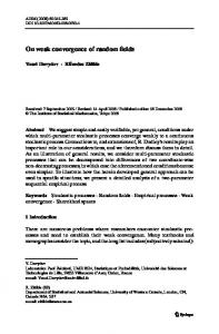
(c) Figure 2.1. Air survey experimental results of the disturbed sea surface (Paci®c, Japan Sea). (a) the height of air survey is 500 m; (b), (c) the height of air survey is 3000 m. The spatial distance between (b) and (c) frames is 20 km.

If we consider the processes progressing both in space and in time, …x; y; t†, then in this case we imply the random (or stochastic) ®elds. A remarkable example of a spatial-temporal random ®eld is the well-known sea disturbance (Figure 2.1(a)), which represents a continuously changing ®eld of elevations over the average level. A lot of serious experiments have shown that sea disturbance (at various stages of its development) represents a virtually ideal random process (of Gaussian type), when it is considered both in space (the random three-dimensional ®eld) and in time, for example, at the same measurement point (the random time signal or the time series). When the source of illumination ± the Sun ± changes its position with respect to a recording device on the aircraft, the situation drastically changes. The quasire¯ecting stochastic surface converts the image of an almost point-like source (remember that the angular dimension of the Sun equals 30 minutes of arc) into the ¯uctuating ®eld of patches of sunlight, which is just recorded by the remote sensing device at some particular time instant (Figure 2.1(b)). In surveying another time instant the ®eld of patches of sunlight will be, certainly, di€erent, i.e. another (and independent) ensemble of the ®eld of patches of sunlight will take place. However, in this case some speci®c large-scale characteristics of the ®eld of patches of sunlight (the elliptical pattern, its characteristic dimensions ± the axes of

40

Random signals and ®elds

[Ch. 2

an ellipse) will be strictly conserved. The characteristic dimensions (angular or spatial) of a random ®eld of patches of sunlight are closely associated with statistical characteristics of the ®eld of elevations of the sea surface (and, more speci®cally, of the ®eld of slopes) and, accordingly, with characteristics of the disturbance (the sea force, the near-surface wind velocity). In the context of optical survey, performed from a low-altitude (500 m) aircraft (Figure 2.1(a)), a large sea wave breaking in the form of a crest foam package is observed. As we shall see below (Chapter 12), the ®eld of breaking gravitational waves also represents the ideal random process to some extent, but of a quite di€erent, Poisson point-like, type. 2.2.1

Ensembles of realizations

Dealing with the deterministic signals, we can map them in the form of functional time dependence, where one particular process has a single realization. In the case of random processes the situation is much more complicated. Fixing instantaneous values of a random signal on a particular time interval, we obtain one of the possible realizations of this random process. The distinction from determinate signals is paramount here. The fact is, that in its complete form the random process is expressed via the in®nite combination of such realizations, which form a statistical ensemble. Such an ensemble can represent a system of noise signals f1 …t†; 2 …t†; . . . ; k …t†; . . .g, which can be observed simultaneously at outputs of completely identical ampli®ers (without a determinate input signal). The intrinsic (and non-removable in any circumstances) noises of radio equipment are called Nyquist noise. A schematized version of such a model experiment is shown in Figure 2.2(a). There is no problem in carrying out such an experiment at the modern technological level of manufacturing radio-engineering systems. The example of experimental noise signal recording at an output of a solitary radio instrument is presented in Fig 2.2(b). Another example is the set of data on measuring sea roughness heights obtained from in situ height measurement instruments spaced at very large distances from each other. Such measurements no longer have a model character; they actually yield serious results. From a purely external point of view, sea roughness height recordings obtained at one measurement point look like just as shown in Figure 2.2(b). The noise type of a signal, received from radio instruments and from sea roughness measurements, is (surprising as it may seem) the same ± the Gaussian process (see below). Examples of realizations of the three-dimensional ®eld of slopes of the sea surface, obtained at the ®xed time instant but under various illumination conditions, are presented in Figure 2.1(a), (b). 2.2.2

Probability densities of random processes

Let …t† be the random process speci®ed by an ensemble of realizations, and t1 be some arbitrary time instant. Fixing the values of random processes at this instant

Sec. 2.2]

2.2 Basic characteristics of random processes 41

Figure 2.2. Simpli®ed scheme to generate the statistical ensemble for the random process (electrical noise example). (a) The set of identical ampli®ers with noise output signals (the qualitative presentation). (b) Experimental time series of output noise normal signal for the individual high-sensitive microwave radiometer. Time and intensity scales (in kelvins) are shown on abscissa and on ordinate.

for the whole ensemble f1 …t1 †; 2 …t1 †; . . . ; k …t1 †; . . .g simultaneously, we obtain the one-dimensional cross-section of the given random process …t1 †. Here the important characteristic is introduced, p…; t1 †, which is called the one-dimensional probability density function, or the density function …t† at time instant t1 . The physical signi®cance of this important characteristic is as follows: quantity

42

Random signals and ®elds

[Ch. 2

P… < …t1 †   ‡ d† ˆ p…; t1 † d is the probability of the fact, that the realizations of a random process at time instant t1 will assume the values lying in the range …;  ‡ d†. An integral analogue for the probability density is the distribution function of a random quantity, which is equal to the probability that the random values …t1 † will assume values equal to, or smaller than, some particular : F…; t1 † ˆ Pf…t1 †  g:

…2:1†

And, accordingly, the density function is determined as the derivative of the distribution function: p…; t1 † ˆ dF…; t1 †=d: …2:2† The probability density possesses the following basic properties: (1) The probability density is non-negative (the positive de®niteness condition), i.e. p1 …†  0. (2) The probability of a random quantity falling in the range of …1 ; 2 † is equal to the integral of the probability density within these limits: … 2 P ˆ f1   < 2 g ˆ p1 …† d ˆ F…2 † F…1 †: …2:3† 1

(3) The integral within the in®nite limits of function p1 …† is equal to unity (the normalization condition): … 1

1

p1 …† d ˆ 1:

…2:4†

In the theory and practice of random processes (including remote sensing tasks), of fundamental importance is the Gaussian (normal) one-dimensional probability density: " # 1 p1 …† ˆ p exp 2

…

m†2 ; 22

…2:5†

which is determined by two numerical parameters m and . The corresponding plot represents the well-known symmetrical bell-shaped curve with a single maximum at point m and exponentially falling tails of distributions. When parameter  decreases, the density function tends to be localized in the vicinity of point m. The physical signi®cance of parameters is obvious enough: parameter m is the mean value of a random quantity, and parameter 2 , called a variance, characterizes the degree of `dispersion' of random values of the process under study around the mean value. In the normal distribution the probability of a random quantity falling in the given interval …; † is: P…    † ˆ ‰… where 1 …z† ˆ p 2

…1 1

exp

m†=Š

‰…

m†=Š;

! x2 dx; … z† ˆ 1 2

…z†;

…2:6† …2:7†

Sec. 2.2]

2.2 Basic characteristics of random processes 43

is the tabulated probability integral. It follows directly from this condition, that the probability of the fact that the signal falls in the interval between the values of m  and m ‡ , equals 0.683. And, on the other hand, the Gaussian signal almost always (with a probability of 0.9973) lies within the interval between m 3 and m ‡ 3 (the so-called `three sigma rule'. This circumstance has often (and successfully) been used in experimental practice, as we shall see below (Chapter 3). You should not, however, think, that the normal distribution possesses some unique intrinsic universality. There are a lot of distributions which appear in quite diverse problems, including those of a geophysical, hydrodynamic and radio-physical type, and possess not lower universality than the normal distribution, such as Poisson's distribution, Rayleigh's distribution and the binomial distribution (Feller, 1971; Rytov, 1966; Zolotarev, 1983; Mandel and Wolf, 1995). A remarkable example in this respect is the turbulence phenomenon in various physical media, in the atmosphere, in the ocean and in plasma media. In spite of the fact, that some turbulence properties are close to Gaussian ones, in general turbulence represents an essentially non-Gaussian process, because otherwise the internal ¯ow (Richardson±Kolmogorov's cascade) of energy over various scales would be absent. It is the functioning of such an energy cascade in a fairly complicated, alternating regime which provides the existence of turbulence as a widespread physical phenomenon (see, for instance, Monin and Yaglom, 1971; Frisch, 1995; Anselmet et al., 2001). Another interesting example can be the studies of statistical properties of the time sequence of the intensity of a global tropical cyclogenesis, namely, the discovery of the Poisson character of some its properties in the limited time scale. In general, however, the global cyclogenesis process principally di€ers from the Poisson-type process in the existence of complicated internal hierarchic correlation links, since in the opposite case (i.e. in a purely Poisson regime) the de®nite stability and cyclic character of temporal functioning of this process would not be provided (Sharkov, 2000). The physical signi®cance of one-dimensional probability density is rather transparent: this is the distribution of instantaneous amplitudes of the process, obtained by mapping the whole statistical ensemble at a ®xed time instant. Thus, this characteristic, while providing information on amplitude features of the process, is mainly insucient for obtaining information on the character of process development in time (or in space). New information about the internal temporal (or spatial) relationships of the process can be obtained by making two cross-sections of a random process at non-coinciding time instants t1 and t2 . The two-dimensional random quantity arising in such a mental experiment which is extracted from the ensemble of realizations, f…t1 †; …t2 †g, is represented by the two-dimensionial probability density p…1 ; 2 ; t1 ; t2 †. This characteristic allows us to calculate the probability of the event involving the fact that the realization of a random process at t1 takes place in the vicinity of point  ˆ 1 , and at t ˆ t2 in the vicinity of point  ˆ 2 . This results in the principal distinction of this two-dimensional characteristic from the onedimensional probability density, namely, the two-dimensional probability density contains information on the internal correlation links of a process.

44

Random signals and ®elds

[Ch. 2

The evident further generalization is the n-dimensional cross-section of a random process …n > 2† leading to the n-dimensional probability density pn …1 ; 2 ; . . . ; n ; t1 ; t2 ; . . . ; tn †. The physical signi®cance of this characteristic is rather complicated now: here we deal with the n-dimensional correlation internal links in the process. The multidimensional probability density should satisfy the conventional conditions imposed on one-dimensional densities, as well as the condition of symmetry. This means that the density should not change at any re-arrangement of their arguments. And, moreover, the multidimensional probability density should satisfy the condition of coherence, which means that, knowing the n-dimensional density, it is always possible to ®nd the m-dimensional density, for m < n, by integrating over the `super¯uous' coordinates. The multidimensional probability densities of comparatively high dimension make it possible to describe the properties of random processes in a great detail. So, the multidimensional process …t†, which depends on a single real parameter t (time), is considered to be completely de®ned over the interval …0; T†, if for arbitrary number n and for any time instants t1 ; t2 ; . . . ; tn the n-dimensional probability distribution density pn …1 ; 2 ; . . . ; n ; t1 ; t2 ; . . . ; tn † is known over this interval. However, the experimental determination and studying of multidimensional (except for onedimensional) densities is a fairly complicated (and often insolvable) problem. 2.2.3

Moment functions of random processes

In some cases, for the solution of experimental and practical problems related to studying random processes it is sucient to consider simpler characteristics of integral type, called the moments of those random quantities, which are observed at cross-sections of these processes. Since in the general case these moments may depend on time arguments, they are called moment functions. As in the case of densities of distributions, it is possible to generate the n-dimensional moment function. However, being within the framework of the so-called spectral-correlation approach, we shall consider only three moment functions of lower orders which, nevertheless, will ensure (as we shall see below) signi®cant progress in the understanding and quantitative description of energy characteristics of a random process. The one-dimensional initial moment function of the ®rst order, …1 Mf"…t†g ˆ m1 …t† ˆ p1 …; t† d ˆ …t†; …2:8† 1

is called the mathematical expectation (the mean value or the ensemble average) of a random process at the current time instant t. Note that the averaging is performed here over the whole ensemble of realizations, and this value is, generally speaking, di€erent for di€erent time instants. The one-dimensional central moment function of the second order is de®ned as …1 2 2  …t† ˆ Mf‰…t† m1 …t†Š g ˆ ‰…t† m1 …t†Š2 p1 …; t† d; …2:9† 1

and called the variance of a process ± the parameter determining the degree of

Sec. 2.2]

2.2 Basic characteristics of random processes 45

scattering of instantaneous values that the separate realizations of the process assume at the ®xed cross-section. Disclosing the square at the right-hand side and taking the integral, we obtain the important relationship we shall use many times hereafter: 2 …t† ˆ Mf2 …t†g m21 …t† ˆ 2 …t† ‰…t†Š2 : …2:10† The two-dimensional initial moment function of the second order, …1 …1 Mf…t1 †; …t2 †g ˆ 1 2 p2 …1 ; 2 ; t1 ; t2 † d1 d2 ˆ B…t1 ; t2 †; 1

1

…2:11†

is called the correlation function of a random process …t†. This function characterizes the degree of statistical coupling of those random quantities, which are observed at t ˆ t1 and t ˆ t2 . In other words, the integral is taken over two separate realizations of a random process at non-coinciding time instants. The physical signi®cance of a correlation function can hardly be overestimated ± it contains the whole information on the intensity of the process, which is required for an overwhelming majority of investigations. The consideration based on the use of a correlation function is called the spectral-correlation approach (see, for example, Davenport and Root, 1958; Kharkevich, 1962; Rytov, 1966; Bendat and Piersol, 1966; Cressie, 1993). Certainly, this approach does not cover all the ®ner features of random process functioning. So, for example, such an approach fails to reveal the spatial-temporal hierarchy of interactions in complicated natural processes, such as the global climate, the El NinÄo phenomenon and the global tropical cyclogenesis (IPCC, 2001; Beniston, 1998; Diaz and Margraf, 1993; Tziperman et al., 1997; Navarra, 1998; Sharkov, 2000). But, nevertheless, the spectral-correlation approach has been successfully used for the description of the general energy characteristics of a process. Such a consideration is quite sucient for a number of problems in radio physics and remote sensing, as we shall see below. 2.2.4

Stationary random processes

An important class of random processes is represented by the stationary random processes, i.e. those random processes whose statistical characteristics are invariable in time. The random process …t† is called stationary, in a narrow sense, if all its probability distribution densities pn …1 ; 2 ; . . . ; n ; t1 ; t2 ; . . . ; tn † of arbitrary order n do not change, when all points t1 ; t2 ; . . . ; tn are simultaneously shifted along the time axis for any time shift . Stationary, in a broad sense, is such a random process, …t†, whose mathematical expectation Mf…t†g and variance do not depend on the current time, and whose correlation function B…t1 ; t2 † depends only on the di€erence (lag)  ˆ jt1 t2 j between time instants under consideration, i.e. B…t1 ; t2 † ˆ B…†. It is clear that the stability in a broad sense follows from the stability in a narrow sense, but not the opposite. Both these notions of stability coincide for the Gaussian process, since the stationary Gaussian process is completely determined by the mathematical expectation and correlation function of the process. In other words, the mathematical expectation and correlation function allow us to calculate

46

Random signals and ®elds

[Ch. 2

any multidimensional probability density of the stationary Gaussian random process. The one-dimensional density is given by formula (2.5), and two-dimensional density is determined by the following relation: p2 …1 ; 2 † ˆ

1 p 2 1 R2 …†  1 p  exp 2 2 1 R2 …† 2

 ‰…1

m†

2

2R…†…1

m†…2

m† ‡ …2

2



m† Š ;

…2:12†

where 2 is the variance of the process, and R…† ˆ ‰B…† m2 Š=2 . Pay attention once again to the fact, that, unlike the one-dimensional distribution density, the two-dimensional density contains mainly new information about the correlation (spatial or temporal) properties of the process. Thus, processes with completely di€erent internal correlation properties can have Gaussian onedimensional distribution (in magnitude). 2.2.5

Ergodic property

The stationary random process is called ergodic if, in ®nding any statistical characteristics, the averaging over a statistical ensemble with the probability of unity is equal to a time-averaged characteristic, taken over any single realization of the process. In this case the averaging operation is performed over a single realization of the process whose length, T, tends to in®nity. Designating time-averaged values by an overbar, we can write the ergodicity condition as follows: …T Mf…t†g ˆ …t† ˆ lim …1=T† …t† dt; …2:13† T!1

B…† ˆ M‰…t†…t

0

†Š ˆ …t†…t

† ˆ lim …1=T† T!1

Note at once, that 2

2

B…0† ˆ M‰ …t†Š ˆ  …t† ˆ lim …1=T† T!1

…T 0

…T 0

…t†…t

2 …t† dt:

† dt:

…2:14†

…2:15†

Thus, the variance of the ergodic stationary process is equal to D…† ˆ 2 ˆ M…2 †

M 2 …† ˆ 2 …t†

‰…t†Š2 ˆ B…0†

M 2 …†

…2:16†

The relation obtained for ergodic processes absolutely corresponds to the similar equality obtained for characteristics of random processes in their averaging over the statistical ensemble (2.10). In order that the random process be ergodic, it should, ®rst of all, be stationary in a broad sense (the necessary condition). The sucient condition of ergodicity is

Sec. 2.3]

2.3 Fundamentals of the correlation theory of random processes 47

the tending to zero of the correlation function (with subtraction of a constant component) with the unlimited growth of time lag: lim fB…†

!1

m2 g ˆ 0

…2:17†

Detailed mathematical analysis has shown that these requirements can be essentially `softened', and the class of ergodic processes can be expanded (see, for instance, Rytov, 1966; Monin and Yaglom, 1971; Frisch, 1995). The concept of ergodicity can be transferred from time to space and to performing any determinate operation with a random process (Monin and Yaglom, 1971; Rytov et al., 1978; Frisch, 1995). So, the stationary ®eld …t; x; y; z† ˆ …t; r†, as a function of time and three coordinates, is ergodic if we suppose that for an arbitrary determinate function the following equality is almost certainly valid: …T h f ‰…t; r†Ši ˆ lim …1=T† f ‰…t; r†Š dt; T!1

0

where the angle brackets imply averaging over the statistical ensemble with the density function, which will correspond to the determinate transformation (see section 2.5 below), and the time T of averaging over the temporal realization should essentially exceed the characteristic correlation times of the process (see section 2.3). Along with ergodicity in time, we can introduce the notion of spatial and spatial-temporal ergodicity. So, for homogeneous, spatially ergodic ®elds the ensemble-averaged values in a sense of convergence in probability are equal to spatial-averaged values. This actually means that for the arbitrary determinate function f the following equality can be considered to be valid: …V h f ‰…t; r†Ši ˆ lim …1=V† f ‰…t; r†Š d3 r; V!1

0

where V is the spatial domain, over which the spatial averaging is carried out. The limiting transition V ! 1 can be stopped on spatial domains whose size is great as compared to characteristic correlation features of the statistical ®eld (see section 2.3). The concept of the spatial-temporal ergodicity of stationary and homogeneous ®elds is applied in cases where the convergence over the ensemble takes place both for T ! 1, and for V ! 1, i.e. when the aforementioned equalities are ful®lled simultaneously.

2.3

FUNDAMENTALS OF THE CORRELATION THEORY OF RANDOM PROCESSES

Along with a complete description of random process properties by means of multidimensional probability densities, another approach is also possible, where the random processes are characterized by their moment functions. The theory of random processes, based on using the moment functions of the second order and

48

Random signals and ®elds

[Ch. 2

lower, was called the correlation theory (or the spectral-correlation approach). As we have noted above, the undoubted advantages of such an approach consist, ®rst, in a fairly complete description of the energy characteristics of a stochastic process, which is quite sucient for the solution of basic problems in many applications. And, second, such an approach provides a reliable experimental methodology and instrumental basis for measurement procedures using random processes. A similar conclusion cannot be drawn (at least for today) for the approach that uses multidimensional densities of statistical ensembles. 2.3.1

Basic properties of the correlation function

The correlation functions of stationary ergodic processes possess some important properties which are widely used in experimental and observational practice: (1) As follows from the de®nition of a stationary random process, function B…† is even: B…† ˆ B… †. (2) The absolute magnitude of the correlation function of a stationary random process for any  cannot exceed its values for  ˆ 0: jB…†j  B…0† ˆ D…† ‡ ‰…t†Š 2 : (3) As  increases without limit, function ‰B…† m2 Š tends to zero (the suf®cient condition of ergodicity), i.e. lim!1 ‰B…† m2 Š ˆ 0. It is very important to understand the physical signi®cance of the correlation function of a random process. For this purpose, let us imagine that the random process …t† under consideration is some ¯uctuating voltage supplied to the active resistance with numerical value of one ohm. According to the Joule±Lenz law, the time-averaged value of the square of the voltage is equal to the amount of heat which is released in such a conductor per unit time (one second). Thus, in the physical sense, B…0† ˆ ‰2 …t†Š is the total power of the ¯uctuation process, and ‰…t†Š2 is the power of a constant component of the process. Remembering relation (2.16), we can easily grasp that the variance of a random process characterizes the power of the ¯uctuation component of a process. We shall repeatedly return to such a convenient physical treatment of the correlation function, since it allows us to understand the physical peculiarities of phenomena in many complicated situations. 2.3.2

The correlation coef®cient

To eliminate the amplitude characteristics of the process and to reveal its purely correlation properties, we introduce the notion of a normalized correlation coecient R…†: R…† ˆ ‰B…† B…1†Š=‰B…0† B…1†Š ˆ ‰B…† …†2 Š=2 : …2:18† In accordance with the properties of the correlation function listed above, the correlation coecient has a form of either monotonously decreasing function or attenuating oscillating functions, and for  ˆ 0 the correlation coecient of any

Sec. 2.3]

2.3 Fundamentals of the correlation theory of random processes 49

random process is always equal to unity. Note that it is of great importance, on the one hand, to determine the character of decreasing of the coecient for large values of shift and, on the other hand, to ®nd the speci®c shape of the `nose' of a correlation coecient for  ! 0. The latter feature determines the small-scale (pixel) structure of the process, whereas the large-scale structures of the process are characterized by the form of the correlation coecient for large shifts. Since the correlation coecient is even, its values are considered for positive shifts (lags) only. The degree of correlation of a random process can be characterized by the following numerical parameter, the interval (or time) of correlation k , which is determined as follows: …1 k ˆ jR…†j d: …2:19† 0

Geometrically, the correlation interval is equal to the base of a rectangle with a height equal to unity, whose area is equal to the area included between the jR…†j curve for  > 0 and the abscissa axis. In some cases, the correlation time means the value of  for which the ®rst intersection of zero takes place. The value of k gives a rough idea of over which time interval, on average, the correlation between the random process values takes place. Slightly simplifying the situation, we can say that the probabilistic forecasting of the behaviour of any realization of a random process is possible over time spans smaller or of the order of time k , if the information on its behaviour `in the past' is known. However, any attempt to accomplish forecasting for the time essentially exceeding the correlation interval will be abortive: the instantaneous values, in time spans essentially greater than the value k , are virtually uncorrelated; in other words, the mean value of the product …t†…t ‡ † is close to zero. 2.3.3

The statistical spectrum

The spectral theory of deterministic signals is well known. However, the probabilistic character of separate realizations of a random process makes it impossible to transfer the methods of spectral analysis of determinate signals directly (straightforwardly) into the theory and practice of random processes. If we calculate the spectral density of a random process …t† by the standard formula of the Fourier integral. …1 _ S…!† ˆ …t† exp … j!t† dt; …2:20† 1

_ then the complex function obtained, S…!†, will be a random function and, moreover, it could not exist at all, generally speaking. We shall obtain here the result, which can be called a spectrum of one of possible realizations of the random process. Under conditions of real observation of some random process proceeding during time T, we can really obtain the current spectrum of the given realization, i.e. the complex function S_ T …!†: …T _ …t† exp … j!t† dt: …2:21† ST …!† ˆ 0

50

Random signals and ®elds

[Ch. 2

However, if we consider various realizations of the random process …t† of ®nite duration T, then for them the complex function S_ T …!† will vary in a random manner from one realization to another, not tending to any ®nite limit at T ! 1, in the general case. Thus, it is desirable to introduce such spectral concepts, which would lead to non-random (deterministic) functions, and then to use the procedures that are methodologically close to the Fourier spectral procedures. In developing the spectral methodology suitable for analyzing random processes, of principal signi®cance is the mathematical theorem proved by the well-known mathematicians, A. Ya. Khintchin and N. Wiener, which is known now as the Wiener±Khintchin theorem. According to this theorem, the correlation function B…† can be presented as …1 B…† ˆ exp … j!† dF…!†; …2:22† 1

where F…!† is a non-decreasing limited function. If function F…!† is di€erentiable, designating ‰dF…!†=d!Š ˆ 12 G…!†; we obtain, instead of (2.22), B…† ˆ

1 2

…1 1

G…!† exp … j!† d!:

…2:23†

Thus, the nearly introduced function G…!† is nothing other than the usual Fourier transformation for the correlation function: … 1 1 G…!† ˆ B…† exp … j!† d: …2:24†  1 Function G…!† is just what is called the statistical spectrum of a random process (Wiener's spectrum), and formula (2.24) is the main de®nition of this function. It should be noted, that both B…†, and G…!† are even functions of their arguments. As a result, relations (2.23) and (2.24) can be written in the real form of two Fourier cosine-transformations: … B…† ˆ

1

0

2 G…!† ˆ 

G…!† cos …!† d!;

…1 0

B…† cos …!† d:

…2:25† …2:26†

The physical signi®cance of functions …t† and G…!† can easily be clari®ed by letting  ˆ 0 in (2.25). Using this procedure, we obtain …1 B…0† ˆ P ˆ G…!† d!: …2:27† 0

Remembering the physical signi®cance of the correlation function for  ˆ 0 as a total power of process P, it can easily be understood that function G…!† expresses the

Sec. 2.3]

2.3 Fundamentals of the correlation theory of random processes 51

power of process …t† falling on the frequency band d! in the vicinity of selected frequency !. In other words, function G…!† represents the spectral density of power. On this basis G…!† is called the power spectrum (or Wiener's spectrum) of process …t†. By its physical signi®cance the power spectrum is real and nonnegative, G…!†  0. This property, however, imposes rather strict limitations on the form of admissible correlation functions: so it follows from relation (2.25), that the correlation function of a stationary process should satisfy the additional (to the three aforementioned ones) condition …1 B…† cos …!† d  0: …2:28† 0

So, principally inadmissible is the approximation presentation of a correlation function in the form of rectangle, i.e.  B0 jj < 0 B…† ˆ ; 0 jj > 0 since in this case the corresponding power spectrum will have negative values, and condition (2.28) is not satis®ed either. It is interesting to note that functions of the type exp f n g are also unsuitable for approximations of B…†, except for the Gaussian curve and exponent …n ˆ 1; 2†. We shall encounter these circumstances below in analysing particular forms of spectra. As to the power spectrum dimension, it completely depends on the physical character of a random process. So, if the random process is the electrical voltage, then its power spectrum, according to relation (2.25), has dimension [V 2 sec/rad]. If, however, the stochastic behaviour of sea disturbance is investigated, then the power spectrum of ¯uctuating altitudes has dimension [m2 sec/rad]. We shall not forget here that the circular frequency ! has dimension [rad/sec] and is associated with frequency … f †, measured in hertz, by the relation ! ˆ 2f . In applications the necessity often arises to consider the behaviour of a random process and, in particular, its energy characteristics within the limited frequency band …!1 ; !2 †. In this case the power of the process P12 , concluded within the ®nite band between !1 and !2 , can be determined by integrating G…!† within corresponding limits (for ! > 0): … P12 ˆ

!2

!1

G…!† d!:

…2:29†

In addition, it is necessary to have in mind that the experimentally measured power spectrum is taken over positive frequencies only. Thus, in experimental practice the notion of one-sided power spectrum is introduced. This spectrum GS … f † represents the mean power of the process fallen per unit frequency band of width 1 Hz:  2G…2f † for f  0 GS … f † ˆ : 0 for f < 0 The one-sided power spectrum has dimension which di€ers from the dimension of a total power spectrum. So, for the process associated with the electric voltage, the

52

Random signals and ®elds

[Ch. 2

dimension of the spectrum will be ‰V 2 =HzŠ, and for the spectrum of sea wave heights it will be [m2 /Hz]. Thus, the total power of the process can be written as …1 …1 B…0† ˆ G…!† d! ˆ GS … f † df : 0

0

For further analysis it is important to ®nd the relationship between the statistical spectrum and the current spectrum of any realization. We take advantage of the following energy considerations: the total energy of the process, released for time T, will be equal to the following value: … …T 1 1 _ ET ˆ 2 …t† dt ˆ jS …!†j2 d!:  0 T 0 This relation expresses the Parseval identity for the ®nite time interval T (see Appendix B). The average power of the process PT for time T is obtained by dividing the value of energy for interval T by its value: … ET 1 1 _ ˆ PT ˆ jS …!†j2 d!: …2:30† T 0 T T This quantity depends, generally speaking, on the value of interval T, but for a stationary and ergodic process it tends, with increasing T, to the constant limit, which just expresses the power of the process: …1 1 P ˆ lim PT ˆ lim …1=T† jS_ T …!†j2 d!: …2:31† T!1  T!1 0 Exchanging the places of integral and limiting procedures and comparing (2.31) with (2.27), we see that the statistical spectrum is related to the current spectrum by the important equation 1 G…!† ˆ lim …1=T†jS_ T …!†j2 : …2:32†  T!1 The analysis of this relation allows us to draw the following important conclusion. The power spectrum of a stationary random process, being always real, does not bear any information on phase relations between separate spectral components. This makes it impossible to restore any individual realization of a random process from the power spectrum. In other words, the well-known theorem of uniqueness of the spectral analysis of determinate signals (`one spectrum: one realization') has no place in the analysis of stochastic signals. So, it is possible to ®nd a set of various random functions (for example, by transforming the phase spectrum) having the same spectral density and correlation function. Of course, the opposite situation also arises, i.e. the in®nite diversity of time sequences of random processes may correspond, generally speaking, to a single power spectrum. In a number of applications the necessity arises of separating the mean (constant) value from a random process, or, in other words, of performing the

Sec. 2.4]

2.4 Quasi-ergodic processes 53

procedure of centring the initial process 0 …t† ˆ …t† m. In such a case the correlation function of a centred stationary process B0 …† will be equal to: B0 …† ˆ B…†

m2 ;

…2:33†

and the spectral density G0 …!† of a centred process will be as follows: G0 …!† ˆ G…!†

m2 …!

0†;

…2:34†

where by symbol …!† is meant the delta-function with its well-known formal presentation … 1 1 exp ‰ j…! !0 †tŠ dt: …2:35† …! !0 † ˆ  1 In such an approach (which is often used in practice) the constant component of the process is treated as a spectral component with the wavelength equal to in®nity (or with the frequency equal to zero). For m ˆ 0 both spectral density presentations coincide; therefore, hereafter the distinctions in these characteristics will be noticed in the case of necessity only. In physical experiments the situation fairly often arises where the random signal is functioning together with a purely determinate one; so, the windy sea disturbance as a random ®eld is often developed against the background of almost harmonic swell. Whereas it is quite dicult to separate directly each component on time realizations of the total process, this procedure can be fairly easily performed (i.e. the random process can be centred against the harmonic component background) by using the spectral-correlation approach. Thus, it is necessary to construct the correlation function and the power spectrum for the process 0H …t† ˆ …t† A cos !0 t. Using the ergodicity properties (2.14), we obtain the expression for the sought correlation function B0H …† as …2:36† B0H …† ˆ B…† A2 cos !0  and, accordingly, the spectral density G0H …!† of the process, centred on the harmonic component, is equal, taking into account (2.35), to G0H …!† ˆ G…!†

A2 …!

!0 †:

…2:37†

The continuation of the procedure consists in the band ®ltering (and in the elimination, if necessary) of the spectral component found. 2.4

QUASI-ERGODIC PROCESSES

In actual physical practice, the overwhelming majority of processes proceed in regimes that cannot be called purely ergodic. This is due to the fact that any chaotized processes subject to investigation are limited physically both in time and in space. But it is this spatial-temporal limitation, inside which it is necessary, as a rule, to study the behaviour (or evolution) of the system by determining the variation of characteristics of the process, such as its mean value or the change of the noise intensity level in a system (i.e. the value of variance). Situations are often also

54

Random signals and ®elds

[Ch. 2

possible where the spatial-temporal ®eld is ergodic only for a part of spatial arguments, for example, only on the plane …x; y† or in a part of physical threedimensional space. The latter situation often arises in studying the dynamical and radiation properties of the Earth's atmosphere, as well as the dynamical state of the ocean surface. Furthermore, if the spatial ®eld is periodic in spatial variables (coordinates), then the mean value over the spatial periodicity cell will give a poor approximation to the mean value over an ensemble, if the period is not too great compared to the correlation scale. There are also such physical processes that ergodic concepts cannot be applied to straightforwardly. So, it is important to note, that there is no accurate ergodic theorem for groups of rotations in a space (for example, for spiral vortices in the atmosphere), since the rotation can be accomplished by ®nite angles only (Frisch, 1995). Therefore, in physical experiments it is important in many cases to use the concept of the quasi-ergodic ®eld, which is in the same relation to ergodic ®elds as the quasi-homogeneous ®elds are to homogeneous ones (Rytov et al., 1978). The physical signi®cance of such an approach consists in the fact that such ®elds (or temporal one-dimensional processes) are ergodic only in small volumes as compared to characteristic scales L of variation of the ®eld's statistical characteristics (the mean value, variance etc.). It should be noted that it is these variations of a ®eld's parameters which bear the physical load in the study of the physical state and evolution of the ®eld as a physical object. Thus, the region of spatial (or temporal) averaging for quasi-ergodic processes should be compulsorily limited from above by the scale L, but in this case the characteristic size of the averaging region should exceed the characteristic correlation dimensions (spatial or temporal) of the process. Therefore, we can say that the ®eld is quasi-ergodicity only in the case where such an averaging volume V can be introduced that satis®es the two-sided inequality L  V 1=3  lC ;

…2:38†

where lC is the spatial correlation radius. In other words, the averaging volume should be suciently large for the ®eld to experience many spatial ¯uctuations within V and the accumulation could be accomplished. On the other hand, this volume should be small enough, so that within its limits the studied ®elds are fairly homogeneous and the process macro-characteristics do not vary. Similar reasoning can be applied to temporary processes, but in this case the spatial correlation radius should be replaced by the correlation interval. In phenomenological physics, by V is usually meant a `physically in®nitely small volume', which performs, in essence, the same functions as the averaging volume considered above (Rytov et al., 1978). However, attention should be paid to the fact that, despite a seemingly simple form of inequality (2.38), the comprehension of its physical sense meets some diculties in each particular physical experiment. So, in processing experimental natural data the correct understanding and ful®lment of this inequality requires considerable e€orts. The inadvertent merging of scales, presented in inequality (2.38), can involve serious artefacts in the ®nal scienti®c interpretation of results. All nuances of this

Sec. 2.5]

2.5 Types of spectra

55

complicated situation are especially visible in analysing studies on the spatialtemporal characteristics of complicated, natural, chaotized processes, such as atmospheric turbulence (Levich and Tzvetkov, 1985; Hussain, 1986; Tsinober, 1994; Frisch, 1995), ®elds of global and regional precipitations (Lovejoy and Schertzer, 1985; Arkin and Xie, 1994; Davis et al., 1996; Olsson, 1996; Sevruk and Niemczynowicz, 1996; Chang and Chiu, 1997; Jameson et al., 1998; Smith et al., 1998; Lucero, 1998; Andrade et al., 1998; Sorooshian et al., 2000; Simpson et al., 2000), the evolution and stochastic behaviour of the global climate (IPCC, 2001; Ghil et al., 1985; Glantz et al., 1991; Beniston, 1998; Monin and Shishkov, 2000), or the stochasticity of global tropical cyclogenesis (Sharkov, 2000). We shall touch on the quasi-ergodicity issue in di€erent sections of the book as required.

2.5

TYPES OF SPECTRA

The spectral patterns of stochastic natural objects and processes are fairly diverse. Nevertheless, there are some typical features of power spectra (the shape of spectra, the characteristic band of a spectrum, the spectral density moments), which make it possible to classify fairly rapidly and reliably the received experimental data and to obtain the initial model physical ideas about the processes under study. It is the e€ective spectrum width that is most frequently used as a basic quantitative characteristic, namely, … …
! 1 1 1 1
f …Hz† ˆ ˆ GS … f † df ˆ G…!† d!=2; …2:39† 2 GS0 0 G0 1 where subscript 0 denotes the extremal spectral density values. This numerical characteristic is frequently used in experimental practice and engineering calculations, thus making it possible to easily ®nd the variance (power) of a random signal: 2 ˆ GS0
f ˆ 2G0
!. Generally speaking, the e€ective width of a spectrum of the random process can also be determined by di€erent methods, for example, from the condition of power spectrum decreasing at the boundary of this frequency range down to the level of 0:1GS0 . In any case, between the correlation interval k and the e€ective width, some `uncertainty' principle should take place (this term is borrowed from quantum mechanics), namely, …2:40†
f k ˆ const ˆ O…1† that follows from the basic properties of the Fourier transformation. Having determined the e€ective band and correlation interval proceeding from de®nitions (2.19) and (2.39) presented above, we can obtain for symmetrical spectra relative to zero the value of the constant as 14. Thus, the broader the power spectrum of noise, the more chaotic the time variations of its temporal realizations and the smaller the correlation interval value. However, the knowledge of only these parameters of a random process is, in a number of important cases, not sucient for determining the

56

Random signals and ®elds

[Ch. 2

physical features and intrinsic dynamics of the phenomena. Here we can refer to problems mentioned above of studying the internal structure of turbulence, climate stochasticity and global tropical cyclogenesis. Much more insight into the processes is achieved by studying the power spectrum form for the phenomenon under investigation within a wide frequency range. In such a case it is important to know not only the central and maximum parts of a spectrum (or, as is sometimes said, the energy-carrying part of the spectrum), but also the distant (from the extremal value) down-falling tails of a spectrum, which, in their turn, can consist of several branches coupled in a particular succession. It is the parameters of these branches and the succession of their coupling which determine the most important processes of energy transformation in a system, the external energy input to a system and output from it (the dissipation processes, such as transfer into heat). And here again we can point out, as an example, the important features of spectra of velocity ¯uctuations in the turbulent atmosphere (Kolmogorov and anti-Kolmogorov branches), which determine quite di€erent physical processes: the direct (decay) and reverse (selforganization) cascades of energy transfer in a system over spatial scales. Below we shall consider some of the most frequently used approximations of spectral densities and their corresponding correlation functions. 2.5.1

Rectangular low-frequency spectrum

The rectangular low-frequency spectrum represents a spectrum located very close to a zero frequency  G0 j!j 
! G…!† ˆ : 0 j!j >
! The total power of such a model random process will be 2 ˆ 2G0
! ˆ G0S
f . Using formula (2.23), we ®nd the correlation function and then we pass to the expression for the correlation coecient: R…† ˆ sin
!=
!:

…2:41†

It is important to note that the correlation function of the given random process is sign-alternating, and the change of a sign takes place for time shift  that is a multiple of the quantity =
!. This means that, as  increases, the positive correlation between two values of a signal, spaced at , rapidly drops, passes through zero (the absence of any correlation), and then becomes signi®cant again, but with the other sign ± negative in this case. Such a property of the correlation function indicates the quasi-periodicity of any realization of the given random process, which is certainly understood in the probabilistic, rather than in the absolute, sense. It is interesting to note that for the other forms of spectra, which are seemingly close to the form under consideration (see below), such a quasi-periodicity in correlation properties is not observed. When the argument tends to zero, the value of the correlation coecient tends to unity, since the limiting value of function fsin x=xg for x ! 0 equals unity (Gradshteyn and Ryzhik, 2000). By the correlation interval in this case is meant

Sec. 2.5]

2.5 Types of spectra

57

the ®rst value of the argument, for which R…k † ˆ 0. It can easily be seen from (2.41), that k ˆ 14 …
f † 1 . Since the spectral band value is of the order of the central frequency value (we consider the positive frequencies here), such processes are called broadband random processes. Owing to its relative simplicity, the type of a random signal spectrum considered is fairly often used for the ®rst model approximation. Remember, however, that the opposite situation ± the rectangular approximation of a correlation function ± does not take place and is prohibited by the rules of transition between Fourier transforms. 2.5.2

Gaussian spectrum

Suppose the power spectrum of a random signal to be described by the Gaussian function (the quadratic exponent) G…!† ˆ G0 exp … !2 †: To ®nd the correlation function we shall use formula (2.25) and the well-known determinate integral (Gradshteyn and Ryzhik, 2000) R…† ˆ exp …  2 =4 †: …2:42† p p 2 band The total power of the process pwill be  ˆ G0 =2 , the e€ective p  of the process (2.39) will be
f ˆ 14  , and the correlation interval is k ˆ  . In this case the uncertainty relation will be, as would be expected, the value of 14. So, the Gaussian character (Gaussian shape) of a power spectrum results in the correlation function of Gaussian type as well, and any quasi-periodicity in correlation properties is absent in this case. 2.5.3

The Lorentzian spectrum

As we shall see later, natural processes often involve random signals which have a correlation coecient decreasing according to the exponential law R…† ˆ exp … jj†

…2:43†

with some real and positive parameter . Based on (2.26) and using the well-known determinate integrals (Gradshteyn and Ryzhik, 2000), its power spectrum will have the following expression: … 22 1 22 G…!† ˆ ‰=…2 ‡ !2 †Š: exp …† cos ! d ˆ …2:44†  0  It follows from this expression that the power spectrum of the process under consideration has a prominent low-frequency character: the spectral density maximum is observed at zero frequency. In addition, the shape of the spectrum has a peculiar appearance, which is called the Lorentzian spectrum (or the Lorentzian shape). Note also an important feature of the Lorentzian spectrum: as the frequency increases, the drop (the tail) of a spectrum has the typical power-law

58

Random signals and ®elds

[Ch. 2

form 1=!2 . The value of the e€ective band of the spectral density of the given process will be
f ˆ =4, and the correlation interval will be k ˆ 1=. 2.5.4

Band noise

The necessity fairly often arises to approximate a rather narrow spectrum around some central frequency, f0 , i.e. provided that the e€ective band of a noise signal is essentially lower than some central frequency …
f =f0 †  1. Depending on physical processes under study, the value of this parameter (the so-called relative frequency band) can be encompassed within very wide limits ± from 10 2 to 10 8 and lower. Processes of such a type are called narrowband random processes (band noise). The simplest approximation of such a process can be represented as a rectangular spectrum around the central frequency:  G0 !0
!  j!j  !0 ‡
! : …2:45† G…!† ˆ 0 !0
! > j!j > !0 ‡
! This directly leads to the following value of the total power of the process: 2 ˆ 4G0
!, since the total band of frequencies around frequency !0 equals 2
!. However, the form of the correlation function is considerably more complicated in this case. Using formula (2.25) and well-known trigonometric relations, we obtain the following expression for the correlation coecient: R…† ˆ fsin …
!†=
!g cos !0 :

…2:46†

Unlike the form of the correlation coecient for a broadband signal, the narrowband signal possesses internal cosine typing, which re¯ects the fact that the noise signal is as though concentrated around the central frequency and not only can be characterized as a random process, but also can possess quasi-determinate properties. As in the case of broadband signal, the correlation properties can be numerically determined from the ®rst zero value of the correlation coecient's envelope. In this case k ˆ 14 …
f † 1 , where by
f is meant the magnitude of the noise band of a system. This is an important circumstance, since the central frequency value does not e€ect the correlation properties of a noise process. However, as the frequency band narrows, quasi-deterministic properties should be emphasized in more and more detail. To elucidate the physical essence of such a kind of dualism of random processes, we shall consider below two limiting cases: ®rst, when the noise spectral band tends to zero and, second, when the band will grow to in®nity, and the process will possess a smooth spectrum. 2.5.5

Harmonic signal

To obtain such an approximation, we shall tend the spectrum width in expression (2.46) to zero and perform a limiting transition. In such a case we arrive at the model of a random harmonic signal with the correlation coecient R…† ˆ cos !0 :

…2:47†

Sec. 2.5]

2.5 Types of spectra

59

The spectrum corresponds to such a function after the limiting transition in (2.45): G…!† ˆ G0 …!

!0 †;

…2:48†

and the process itself is described by the harmonic function …t† ˆ a cos …!0 t ‡ '†

…2:49†

with the constant (and non-random) amplitude and the phase randomly distributed in the range of 0±2. It should be noted, that such a process is essentially nonGaussian. 2.5.6

White noise

Let us imagine, that the noise band will occupy the entire frequency band: from 1 to ‡1 with the constant value of G0 . In this case, using relation (2.35), we obtain the expression for the correlation function B…† ˆ G0  …

0†;

and, accordingly, R…† ˆ 1 for  ˆ 0 and R…† ˆ 0 for  6ˆ 0. The name of this model of a noise signal is logically contradictory (as is known, the `white' light in optical observations does not possess a smooth, constant spectrum), and the process itself is physically unrealizable, since for it …1 G…!† d! ! 1: B…0† ˆ 2 …t† ˆ 0

Nevertheless, this convenient mathematical model has been widely applied both in theoretical works and in experimental practice. For example, this model can successfully be used when the passband of a circuit (or device) under study, which is a€ected by the external random signal, turns out to be essentially narrower than some e€ective width of its spectrum. Such a process is frequently also called the `delta-correlated' noise. 2.5.7

Coloured noise

As we have mentioned above, in determining the intrinsic dynamics and hierarchic structure of natural stochastic processes and systems, of principal signi®cance are the situations where the power spectrum obeys the power law G…!† ˆ Cj!j n ; C > 0:

…2:50†

The physical signi®cance of spectra with certain particular values of the exponent was found to be so great that the spectra of such a type acquired not only a generalized name, the `coloured' spectra, but also, for particular values of n, their intrinsic names, since they re¯ect various physical processes controlling the energy transformation in a system. The spectrum with the value of n ˆ 5=3 was called Kolmogorov's spectrum (Monin and Yaglom, 1971; Frisch, 1995), and for n ˆ 1; 2 the corresponding random signal was called the `red' noise and `brown' noise. As we have mentioned above, by white noise is meant a signal with the spectrum

60

Random signals and ®elds

[Ch. 2

for n ˆ 0. In recent times such broadband noise, which arises in physical and geophysical systems under the e€ect of external conditions, began to be called, less poetically, `crackling' noise (Sethna et al., 2001; Burroughs and Tebbens, 2001). However, the direct use of spectral-correlation means for studying random processes with such types of spectra does not yield meaningful results. We can easily be convinced of it by taking the integral from the total energy of a process (2.25). Substituting (2.50) into (2.27) we shall see that the integral diverges and, thus, the total power of the process becomes in®nite, which is contradictory from the physical viewpoint. The divergence takes place either at high frequencies (in theoretical works this e€ect is called the ultraviolet* divergence or infrared catastrophe) for n < 1, or at low frequencies (the infrared* divergence or ultraviolet catastrophe) for n > 1, or at both limits for n ˆ 1. This means that the stationary random function with a ®nite variance and power spectrum cannot exist (Frisch, 1995), and, accordingly, the direct use of spectral-correlation means, considered above, for such processes has fairly strict limitations. The physical reason for such an unusual situation became clear only recently. The natural phenomena having power spectra really exist and possess surprising geometrical properties, namely, non-integer geometrical dimension and nondi€erentiability at each point of the process, though the continuity of the process conserves in general and at each point. However, both di€erentiability and continuity conserves for `usual' smooth objects. For these reasons the use of probabilistic moments (the mean values, variances, etc.) and spectral moments is impossible, because they (moments) could not have ®nite values at all, and operations with such quantities are impossible as well. It is a striking fact that it is these natural objects and processes (which have been called self-ane fractals) with peculiar geometrical properties (sometimes called scaling properties), which turn out to be deeply involved in the problems of time forecasting of systems' behaviour and in the problems of transformation of structural properties of systems, such as the transformation of a chaotized system into a more organized structure (the generation of organized vortices in the small-scale turbulence), and, vice versa, the transformation of determinate systems into chaotized ones (the conversion of pendulum-type, near harmonic oscillations into chaotic shivering motions). Multi-year, laboratory, full-scale and theoretical investigations have shown that there exists a large class of natural objects and processes which belong to the `deterministic' chaos, i.e. to some kind of boundary objects between purely determinate systems and `pure' noise processes. It is the objects and processes of such a type which possess surprising geometrical and physical properties (Mandelbrot, 1977, 1982, 1989; Schuster, 1984; Zeldovich and Sokolov, 1985; Glass and Mackey, 1988; Takayasu, 1984, 1988; Kadanov, 1993; Chen and Dong, 1996; Dubois, 1998; Havlin, 1999; Holdom, 1998). In remote sensing problems, such objects include: the rough surface of soils, the geometrical shape of mountain arrays, cloud systems, the geometrical shape of vegetation, ®elds *

These names are purely conventional and, of course, have no relation to the electromagnetic spectrum ranges we have considered in Chapter 1.

Sec. 2.5]

2.5 Types of spectra

61

of atmospheric precipitations, spatial ®elds of humidity of soils and landscapes, spatial ®elds of gravity waves breaking on the sea surface, and the spatial±hierarchic system of river beds (Lovejoy and Schertzer, 1985; Lovejoy and Mandelbrot, 1985; Zaslavskii and Sharkov, 1987; Voss, 1989; Cahalan, 1989; Vasil'ev and Tyu¯in 1992; Vicsek, 1992; Shepard et al., 1995; Davis et al., 1994, 1996; Sharnov, 1996a,b; Gaspard, 1997; Rodrigues-Iturbe and Rinaldo, 1997; Arrault et al., 1997; Hergarten and Neugebauer, 1998; Kothari and Islam, 1999; Dubois, 1998). In radiophysical problems fractal ideology is used in studying the propagation and scattering of electromagnetic waves from rough fractal surfaces (Franceschetti et al., 1996, 1999a,b). Of interest is the fact, that the fractal construction and, accordingly, alternated time behaviour is also characteristic for the systems and objects of biological nature, including the peculiarities of human body architecture, the dynamics of behaviour and even the results of creative activities of a man (Ivanitskii et al., 1998; Havlin, 1999; Ivanov et al., 1999; Taylor et al., 1999). In recent times, however, the problem of the prevalence of fractals in natural phenomena and processes has become the subject of rather strong polemics (Mandelbrot, 1998; Kirchner and Weil, 1998). Slightly simplifying the situation, we can say that the secret of the behaviour of fractals lies in the exponential laws of the behaviour of basic characteristics of systems, such as the dependence of a system's substance mass on its radius, or the dependence of a number of unit elements of a system on the linear scale, or the power spectrum of ¯uctuations in a system (of type (2.50)). It can easily be seen that the exponential law y ˆ Axa …2:51† is equivalent to the following expression: y…x† ˆ a y…x†

…2:52†

for all  > 0. Mathematically, any function y…x† that satis®es Equation (2.52) is called a homogeneous function. A homogeneous function is scale-invariant, i.e. if we change the scale of measuring x, so that x ! x 0 …ˆ x†, then the new function y 0 …x 0 †‰ˆ y…x†Š will still have the same form as the old one y…x†. This fact is guaranteed, since y…x† ˆ  a y…x 0 † according to equation (2.52), and, hence, y 0 …x 0 †  y…x 0 †. The scale-invariance implies that a part of a system is magni®ed to the size of the initial system and this magni®ed part and the initial system will look similar to each other. In other words, there is no intrinsic scale in the initial system. A scaleinvariant system must be self-similar and vice versa. Thus, we see that self-similarity, spatial power laws and scale-invariance are three equivalent ways of expressing the fact that the system lacks the characteristic length scale. It is important to note that the absence of the characteristic time scale in the system leads to temporal power laws (e.g. 1=f noise, the ubiquitous phenomenon in nature). To explain the widespread existence of fractals and scale-free behaviours in nonequilibrium systems, the hypothesis of self-organized criticality has been proposed (Bak et al., 1987), which is supposed to be applicable to many natural and social systems (Larraza et al., 1985;

62

Random signals and ®elds

[Ch. 2

Leung et al., 1998; Kohonen, 1989; Sornette, 2000; Schweitzer, 1997; Tziperman et al., 1997; Rodrigues-Iturbe and Rinaldo, 1997; Hergarten and Neugebauer, 1998; Henley, 1993). In the overwhelming majority of cases the natural objects are not, certainly, purely homogeneous fractals, but they are multi-fractals, i.e. they possess various fractal properties in various scales, or they represent rather complicated conglomerates of purely determinate systems and multi-fractals. In some cases such systems can be represented as so-called non-stationary multi-fractals (Marshak et al., 1994, 1997). Of course, as we have noted above, the direct application of a standard spectral-correlation approach to studying such complicated systems cannot yield meaningful results. To perform such studies, special analytical methods have been developed, which make it possible to analyse the state of a system simultaneously in a very wide range of spatial-temporal scales and to reveal possible inter-scale (and, we should note, nonlinear) interactions. First of all, we should mention here the wavelet-transform methods which have been proposed fairly recently and which are now being developed quite intensively (Chui, 1992; Astafyeva, 1996; Basu and Levy, 1997; Bouman and Newell, 1998). Unlike classical Fourier analysis, the wavelet-transform has a `mobile' time-frequency window that provides information on the evolution of the relative contribution of components at various scales, as the process under investigation develops in time. Thus, the wavelet-transform of a one-dimensional signal results in a two-dimensional ®eld which demonstrates both the frequency-local properties of a basic signal, and their position in the time evolution of a process. This gives rise to the most important feature of the wavelet-transform: the possibility of analysing the temporal dynamics of power transmission at various scales. At present, the wavelet methods are widely used for analysing complicated physical processes where the use of classical Fourier analysis cannot yield satisfactory results. In this respect, we should ®rst of all mention the studies of complicated atmospheric turbulence regimes, which include both Kolmogorov's cascade processes and the formation and existence of coherent structures (Kaspersen and Krogstad, 2001; Terradellas et al., 2001), of convective cloud systems (Yano et al., 2001a,b), the stochastic regime of a global tropical cyclogenesis (Sharkov, 2000), and multi-scale analysis in structure recognition problems on IR and optical images (Frick et al., 2001; Carvalho et al., 2001; Michielsen and De Raedt, 2001). The wavelet-transform can be most eciently used in analysing nonlinear systems where complicated frequency transformations take place, including the generation of new frequencies in a system (Ghanem and Romeo, 2001). More detailed information on the possibilities and techniques of application of the wavelet-transform and similar integralgeometrical methods can be found in papers by Farge et al. (1996), Astafyeva (1996), Bouman and Newell (1998), Frick et al. (2001), and Michielsen and De Raedt (2001). 2.6

LINEAR AND NONLINEAR SYSTEMS AND MEDIA

The natural media through which electromagnetic energy propagates, and the devices used for processing, transforming and transmitting the signals, can be

Sec. 2.6]

2.6 Linear and nonlinear systems and media

63

extremely diverse both in the principles of their intrinsic design and physical properties, and from the viewpoint of their external characteristics. In order to have the possibility of comparing and classifying such media and devices, the concepts are usually formulated using a block-diagram of the `black box' type. The phenomenology of such a type is fairly wide spread in analysing the radiophysical and radiotechnological type of system, as well as the various digital systems in computer systems engineering. The physical signi®cance of such an approach is as follows. No matter how di€erent various radio-technological and digital systems and devices are, we can always distinguish in their structure the input, designed for supplying initial signals, and the output, from which the transformed signals are delivered for further thematic usage. In the simplest case, both the input signal, ui …t†, and output signal, u0 …t†, which is frequently called the response of a system, represent solitary functions of time. A more complicated case (for example, in computer systems engineering) might be the representation of an input signal in the form of an mdimensional vector Ui …t† ˆ ‰ui1 …t†; ui2 …t†; . . . ; uim …t†Š …2:53† and of an output signal, the form of the n-dimensional vector: U0 …t† ˆ ‰u01 …t†; u02 …t†; . . . ; u0n …t†Š:

…2:54†

We should bear in mind that in experimental practice the situation frequently arises, where n 6ˆ m. The law of coupling between signals Ui …t† and U0 …t† is speci®ed by means of the system operator, T, whose e€ect on Ui …t† results in signal U0 …t†: U0 …t† ˆ TfUi …t†tg:

…2:55†

The system operator can be contained inside both arithmetical transformations, and di€erentiation/integration operations, depending on the system's properties. For de®niteness of the problem, it is necessary to specify also the regions of admissible input e€ects (as well as the regions of output signals) in which the system retains its properties. In the simplest case, the question under consideration is the character of input signals (continuous or discrete, determinate or random) and their dynamic range. The major principle of classi®cation of systems (or natural media) is based on the fact that various systems, generally speaking, behave in various manners when a sum of several signals is delivered at the system's input. If the operator of a system is such that the following equalities are valid: TfUi1 ‡ Ui2 g ˆ TfUi1 g ‡ TfUi2 g TfUi1 …t†g ˆ TfUi1 …t†g;

…2:56†

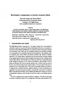
where  is an arbitrary number, then the given system is called linear. The conditions (2.56) express the fundamental superposition principle. The systems (or media) not obeying the superposition principle are called nonlinear. Strictly speaking, all physical systems and media are nonlinear to some extent. It can easily be understood that nonlinearity, as a physical property, is much

64

Random signals and ®elds

[Ch. 2

Figure 2.3. Typical example of amplitude nonlinear characteristic for the radiotechnic ampli®er. ui is the input signal; uo is the output signal.

more general than linearity. However, there exists a great class of systems and media where the linear models that are used for their description yield quite reliable results. As the numerous investigations in this area have shown, linear systems are remarkable due to the fact that for them it is possible to obtain, at least theoretically, the solution of any problem related to the transformation of any input signal. Certainly, the same physical system can operate both as a linear system, and as a nonlinear one, depending on the input signal value. As an example, we may consider the signal of various intensities delivered to an ampli®er, for which the response function (the system operator) has nonlinear character (Figure 2.3). We can easily see in Figure 2.3 that the signal with small amplitude is ampli®ed in a linear manner. At the same time, in the case of the high intensity signal, its form (and its spectral composition) is highly distorted at the system's output. We can also consider a simple (but, as we shall see later, a fundamental) purely nonlinear transformation y ˆ ax2 . At the input of such a device a purely harmonic signal x ˆ cos !0 t with a single spectral component !0 ˆ 2f0 is delivered. Using well-known trigonometric formulas, we shall have at a nonlinear system's output the following signal: y ˆ 12 ‡ 12 cos 2!0 t, or, in other words, the constant component (zero frequency) and the harmonic signal, but with a doubled frequency. It follows from this fact that at the system's output the initial signal has been distorted: we now have the spectral composition, which was completely absent in the initial signal. In other words, the nonlinear system enriches the spectral composition of a signal with new components. The violation of the superposition principle and the distortion of the spectral composition for nonlinear systems is, certainly, not the single principal distinction between linear and nonlinear systems. A lot of nonlinear systems are extremely sensitive to small variations of system parameters and initial conditions. Their

Sec. 2.6]

2.6 Linear and nonlinear systems and media

65

small variation can result in major (`disastrous') consequences: the system can acquire a signi®cantly di€erent time behaviour. An extensive literature is dedicated to elucidating these issues (see, for instance, Lam (1998)). It is the spectral aspect of this problem for systems stable against the change of parameters which will be important for us hereafter. Now we consider the question of the relation between Fourier spectra and characteristics of a system. Suppose that some linear system is speci®ed, which is described by the ordinary di€erential equation of the nth order with constant coecients: dn y dn 1 y dy an n ‡ an 1 n 1 ‡


‡ a1 ‡ a0 y ˆ x…t†: …2:57† dt dt dt We apply the Fourier transformation to both sides of the equation …1 f …t† exp … j!t† dt: 1

…2:58†

On the right-hand side we shall have the spectrum of the function of an input signal x…t†, and for integration of the left-hand side we apply one of basic formulas of spectral analysis (see Appendix B). Then we have " # n X ak … j!†k S_ y ˆ S_ x : …2:59† kˆ0

Here S_ x and S_ y are spectra of functions x…t† and y…t†, respectively. For a polynomial _ j!†. Thus, the spectrum in square brackets we introduce the short designation as Z… of an output signal can be written as S_ … j!† ; S_ y … j!† ˆ x _ j!† Z… and, accordingly, we can write the expression for an output signal: … 1 1 S_ x … j!† y…t† ˆ exp … j!t† d!: _ j!† 2 1 Z…

…2:60†

…2:61†

This formula gives the complete solution of equation (2.57) by the Fourier integral method. In so doing, one more designation is introduced as: _ j!† ˆ K…

1 : _ Z… j!†

…2:62†

This quantity, which expresses the ratio of complex amplitudes at a system's output and input in the harmonic mode, is called the complex frequency characteristic (or the complex transmission coecient) of a system. Formula (2.60) can be written as: _ j!†S_ x … j!†: S_ y … j!† ˆ K… …2:63†

66

Random signals and ®elds

[Ch. 2

It is important to note here that, for practical purposes, the transmission coecient can be fairly simply obtained, in the majority of cases, by means of complex Ohm's law and Kirchho€ 's rules for branched circuits. Using the theorem on the product of spectra (Appendix B), we can ®nd the output signal value in the form of convolution integral (the Duhamel integral) …1 y…t† ˆ x…†h…t † d; …2:64† 1

where h…t† is the Fourier transform of the frequency characteristic of a system that is called the pulse characteristic (pulse response) of a system, or, in other words, the system's response to an input signal in the form of delta-pulse. A great advantage of the Duhamel integral-based analytical technique is the fact that, when the pulse response of a system has been determined, the further stages of solution are reduced to completely formalized procedures. Above we have outlined the methods that enable us to solve any problem related to determinate signals propagation through linear systems. Below we shall consider the methods of transferring these methods into the statistical area for stochastic signals. At the ®rst stage we shall be interested in purely energetic relations only. In this case, remembering the relation for the Wiener spectrum and the current Fourier spectrum (2.32), we can immediately obtain the complete solution of the stated problem within the correlation approach framework. That is to say, the power spectrum of an output random signal is related to a similar spectrum of a signal at an input by means of the following equation: _ j!†j2 Gi …!†; G0 …!† ˆ jK…

…2:65†

and the correlation function at the system's output, according to relation (2.23), will be equal to … 1 1 _ j!†j2 exp … j!† d!: By …† ˆ G …!†jK… …2:66† 2 1 x Remembering relation (2.27), we can ®nd the expression for a variance (or for the energy of a ¯uctuation part) of an output signal as: …1 2 _ j!†j2 d!: y ˆ By …0† ˆ Gx …!†jK… …2:67† 0

As to the distribution densities, the normal processes possess the remarkable property of `stability' with respect to linear (but not to nonlinear) transformations. Moreover, linear systems possess the surprising property of normality of an output random signal, which arises when an input non-normal (non-Gaussian) process has passed through the linear device under the natural condition that the time of correlation of an input process is essentially smaller than the time constant of a linear inertial circuit. Below we shall consider an important example of an inertial integrating linear system, which is frequently used in applications, in particular, in separating a small constant value of a signal against the background of powerful noise.

Sec. 2.6]

2.6.1

2.6 Linear and nonlinear systems and media

67

Low-pass ®lter (LPF)

Experimentally the LPF is constructed as a circuit of a resistor and a capacitor (Figure 2.4(a)). With allowance for the complex Ohm's law we can obtain the expression for the complex transmission coecient of the circuit: 1 _ j!† ˆ u0 …t† ˆ K… ; ui …t† 1 ‡ j!CR

…2:68†

Figure 2.4. Schematic presentation of the functioning of a low-pass ®lter (signal integration electric circuit). (a) Wiring scheme of a low-pass ®lter. (b) Power transmission coecient. (c) Time series of input signal; 0 is statistical average; i is statistical root-mean-square variation (RMS) of input signal. (d) Spectral densities of the input and output signals. (e) Time series of the output signal. o is RMS of the output signal.

68

Random signals and ®elds

[Ch. 2

and, accordingly, the power transmission coecient is _ j!†j2 ˆ jK…

1 ; 1 ‡ !2  2

…2:69†

where  ˆ RC is the circuit constant expressed in seconds. In this case it can easily be seen that the transmission coecient maximum, which is equal to unity, will be located on a direct current (at zero frequency), and then, as the frequency grows, the transmission coecient rapidly drops and accordingly suppresses initial highfrequency components (Figure 2.4(b)). This is the reason that the given circuit was called in such a manner. Let us imagine that at the circuit's input there is a strong ¯uctuation noise ……t†† with a small constant level …0 † of a signal, which just has to be separated and then recorded (Figure 2.4(c)). The spectral characteristics of an input signal can be written in the following slightly simpli®ed form: Gi …!† ˆ …!

0†02 ‡ G0i

…2:70†

and, accordingly, the total power at the circuit's input will consist of a constant component's power and a ¯uctuation component's power: Bi …0† ˆ 02 ‡ 2i ˆ 02 ‡ G0i
!:

…2:71†

Since a circuit's transmission coecient on a direct current is equal to unity, the constant component of an input signal remains unchanged. The ¯uctuation component, however, will undergo qualitative changes. If we have at an input a broadband noise component with the correlation coecient of type (2.41) and correlation time k ˆ 14 …
f † 1 , then at an output of the linear inertial system the spectral characteristics of a signal can be described, as can easily be seen, by the Lorentz-type spectrum (2.44) and correlation properties determined by expression (2.43), i.e. by the descending exponential curve, and with the correlation time equal to the integration constant of a circuit k ˆ RC, which is just what should be expected, generally speaking. The value of an output signal variance can be found by using relation (2.67), substituting into it the values of the transmission coecient on power (2.69). So, using the value of the known integral, we have: …1 d! G  2y ˆ G0i ˆ 0i ˆ G0i
; …2:72† 2 2  2 0 1‡!  where by
is meant the e€ective LPF passband which, accordingly, can be rewritten as
f ˆ 1=…4RC† ˆ 1=…4†. As should be expected, the variance of a noise component of an output signal has sharply decreased, since in this case the band of frequencies, eciently passed by a circuit, has shortened (Figure 2.4(e)). The eciency of separating a constant component of the LPF can be naturally estimated as a ratio of variances of noise components at the circuit's output and input; or, more frequently, the ratio of root mean square (RMS) deviations is used: r 0


1 ˆ ˆ p : …2:73†
! 2
f  i

Sec. 2.7]

2.7 Nonlinear transformations of random processes 69

This can be clearly seen graphically from the comparison of noise `tracks' of a signal at a system's input (Figure 2.4(c)) and output (Figure 2.4(e)) according to the `three sigma' rule. Thus, the eciency of separating a constant component is determined by the ratio of noise bands of input and output signals or by the signal accumulation time. Depending on physical features of observation, the accumulation time can vary within very wide limits, from some tenths of a second up to days. As we shall see soon, the aforementioned ®lter is an indispensable component of noise signal processing in microwave radiation reception systems. At present, the operation considered above is usually performed directly by means of computer procedures.

2.7

NONLINEAR TRANSFORMATIONS OF RANDOM PROCESSES

Nonlinear transformations and, ®rst of all, the quadratic transformation, play a fundamental part in the process of measuring the intensity of a random signal. The fact is that the procedure of measuring the spectral power of a noise signal cannot be constructed as any conceivable combinations of linear systems and circuits (this issue will be considered in more detail below in Section 2.8). The quadratic transformation of a noise signal occurs everywhere where it is necessary to measure the power of a ¯uctuation signal. This conclusion equally relates to the receivers of electromagnetic ¯uctuation radiation in the optical, IR and radiofrequency ranges, for example, the retina of the human eye, photographic devices, IR and microwave radiometers. In analysing the transformation of random processes by nonlinear systems the problem is formulated as follows: supposing the parameters of a system and statistical characteristics of an input process …t† to be known, it is necessary to ®nd the statistical characteristics of a transformed process at an output …t†. As we have already noted, the nonlinear transformation changes both the external time appearance of the initial signal and its spectral composition; and, therefore, both density functions and the correlation function and spectral density of the initial signal also change. In general, the problem of transformation of random signals by nonlinear systems is very complicated; nevertheless, some particular results can be obtained within the framework of a spectral-correlation approach. Suppose  to be the random quantity related with  by a single-valued functional dependence of form y ˆ f …x†. Since the random quantities are interrelated by a single-valued determinate dependence, it can be supposed that from the fact that  lies within a fairly small interval ‰0 ; 0 ‡ dŠ, it certainly follows that quantity  will lie within the interval ‰0 ; 0 ‡ dŠ, where 0 ˆ f …0 †. It follows from this fact that the probabilities of these two events are equal to each other (the property of invariance of the probability di€erential): p…† d ˆ p…†jdj (the modulus has appeared in the expression because the

70

Random signals and ®elds

[Ch. 2

probability density cannot be a negative quantity). Thus, the probability density of a transformed signal will be equal to: d dg …2:74† p1 …† ˆ p1 …† ˆ p1 fg…†g ; d d where g…y† ˆ x is the function reverse to f …x† ˆ y. If the functional relationship between quantities y and x is multi-valued, so that there are several reverse functions (as, for example, in the case of the transformation y ˆ ax2 ), then expression (2.74) is generalized as follows: N X d …2:75† p1 …i † i ; p1 …† ˆ d iˆ1 where N is the number of reverse branches. Using similar probabilistic constructions (namely, the property of invariance of a probability di€erential), we can obtain the following expression for the twodimensional probability density p2 …1 ; 2 †: p2 …1 ; 2 † ˆ p2 fg1 …1 ; 2 †; g2 …1 ; 2 †gjD2 j;

…2:76†

where D2 is the Jacobian of transformation from random quantities 1 ; 2 to random quantities 1 ; 2 : @1 @1 @…1 ; 2 † @1 @2 …2:77† ˆ D2 ˆ : @…1 ; 2 † @2 @2 @1 @2 If we consider the simple case of inertialess (without internal time delays) transformation, where the cross-relations between 1 and 2 and 2 and 1 are absent, then the Jacobian breaks up into the product of derivatives. And, ®nally, from the basic de®nitions of the probability theory we shall have the following expressions for the mathematical expectation and for the second mixed moment (the correlation function) of the transformed process: …1 …1 M1 …† ˆ p1 …† d ˆ f …†p1 …† d …2:78† 1

1

M2 …1 ; 2 † ˆ B…1 ; 2 † ˆ ˆ

…1 …1 1

1

…1 …1 1

1

1 2 p2 …1 ; 2 † d1 d2 ˆ

f …1 † f …2 †p2 …1 ; 2 † d1 d2 :

…2:79†

Further, making use of the basic relation (2.24), we can transfer to spectral characteristics of a transformed signal. Now we consider the important example of the inertialess quadratic transformation y ˆ ax2 …a ˆ 1†, where the normal stationary noise signal with a zero mean

Sec. 2.7]

2.7 Nonlinear transformations of random processes 71

Figure 2.5. Schematic presentation of the functioning of a nonlinear square-law electrical circuit. (a) Square-law function and time series of the input signal. (b) Time series of the output signal. (c) The density function of the output signal.

value …0 † acts on the input of a circuit. Schematically, the whole process of transformation of temporary and probabilistic characteristics is presented in Figure 2.5. Since the function for the transformation under study is doublevalued, then, taking advantage of relation (2.75), we shall have for the density of a transformed signal the following general expression: 8 p p p …  † ‡ p1 … † > < 1 >0 p 2  p1 …† ˆ …2:80† > : 0  > 0; and for 0 ˆ 0 we obtain:

  8 1 y > < p exp 22 22 y p1 …† ˆ > : 0

0

…2:81†

 < 0:

From consideration of (2.81) and Figure 2.5(b), (c) it can be seen that the time character of the transformed signal has radically changed: the values of a signal are only positive. The amplitude dependencies with respect to the initial signal

72

Random signals and ®elds

[Ch. 2

have also sharply distorted: the values of a signal with small amplitudes are considerably suppressed, and the values of a signal with large amplitudes have acquired the shape of sharp spikes. And, what is most important, in the quadratic transformation of a noise signal the constant component has appeared, which just bears the basic information on the power of an initial noise signal. All the above considerations are contained in the amplitude dependence of the density function of a transformed signal (Figure 2.5(c)). Note that the normalization in (2.81), which is necessary for distribution densities, is provided here; i.e., using the known determinate integrals (Gradshteyn and Ryzhik, 2000) we have:   y … 1 exp 1 22 p dy ˆ 1: …2:82† p 2 y 2 0 For the mean value of an output signal, using (2.78) and known determinate integrals (Gradshteyn and Ryzhik, 2000), we obtain the important result ! …1 1 x2 2 M1 …† ˆ  ˆ x p exp …2:83† dx ˆ 2 ; 2 2 2 2x  1 x namely, the mean value (at zero frequency) of the transformed signal is exactly equal to the total power of an input noise signal. However, for many applications it is necessary to know, along with purely amplitude characteristics, the detailed spectral properties of the transformed signal as well. For this purpose it is necessary to correct the spectral character of an initial signal. We shall suppose that the input signal represents a narrowband normal process with spectral-correlation properties presented by relations (2.45) and (2.46), and the two-dimensional density function is determined as (2.12). In this case the correlation function of the transformed output signal will be written as the following integral: …1 …1 1 p B…† ˆ x21 x22 22 1 R2 …† 1 1 ( ) x21 ‡ x22 2Rx1 x2  exp …2:84† dx1 dx2 : 22 …1 R2 † This integral is rather complicated. However, there exists a rather elegant (and nontrivial) substitution that allows us to transform the integral fairly rapidly to a convenient form. Substituting R…† ˆ cos  (since 1 < R…† < 1, then 0 <  < ) and also making the following substitution:   ‡' x1 ˆ 
r cos 2 …2:85†   x2 ˆ 
r cos ' ; 2

Sec. 2.7]

2.7 Nonlinear transformations of random processes 73

we shall have with the help of the Jacobian the transformations of coordinates dx1 dx2 ˆ D2 dr d' ˆ  sin r dr d'; x21 ‡ x22 2 …1

2Rx1 x2 ˆ r2 : R2 †

…2:86†

In this case the variables of integration are separated, and we have the following form of an initial integral: 4 B …† ˆ 

…1 0

5



r exp

r2 2

 dr

… 0

2

cos



     2 ‡ ' cos ‡ ' d' 2 2

…2:87†

and, in the ®nal form, the expression for the correlation function of a transformed process assumes the following elegant form: B …† ˆ 2 …1 ‡ 2R2 …††:

…2:88†

This expression gives rise to some important conclusions. Substituting the value  ˆ 0 into (2.88), we obtain the expression for the total power of a transformed signal B …0† ˆ 34 ˆ 3…  †2 ; …2:89† and in this case the power of a ¯uctuation component (the variance of a transformed signal) is equal to 2 ˆ B …0†B …1† ˆ 24 ˆ 2…  †2 : …2:90† It is interesting to note also, that if the initial signal possesses correlation properties in the form of a symmetric function, i.e. R…† ˆ A…† cos !0 , then the correlation function of a transformed signal (2.88) will be as follows: B …† ˆ 4 ‰1 ‡ A2 …† ‡ A2 …† cos 2!0 Š:

…2:91†

This indicates that, along with a constant component, there are two bands ± the low-frequency band, assigned to a direct current (a zero frequency), and the highfrequency band, assigned to frequency of 2!0 . It is interesting to note that from (2.91) it directly follows that the intensities of noise bands and the value of a constant component of the transformed signal are equal. This follows from the symmetry of the initial problem. However, the complete picture of the spectral density distribution can be obtained only after performing the corresponding Fourier transformation of (2.24) and (2.26). Remembering the expression for the correlation function of a narrowband input noise signal (2.46) and using expressions for determinate integrals (Gradshteyn and Ryzhik, 2000) and for the delta-function (see equation (B.11) in Appendix B), we obtain after some transformations the expression for the spectral density of a

74

Random signals and ®elds

[Ch. 2

Figure 2.6. Transformation of a narrowband spectrum by a square-law circuit. (a) Spectrum of input signal. (b) Spectrum of transformed signal. (c) Spectrum of output signal by low-pass ®lter (LPF). See explanations in the text.

noise-transformed signal ( G …!† ˆ 4 …!

‡

1 …2
!†2

0† ‡

2 …2
!†2

…2
!

!† )

‰…2
!

2!0 ‡ !† ‡ …2
!

2!0

!†Š :

…2:92†

Note, at ®rst, that by
!, as in (2.46), is meant a half of the total band of an input noise signal. Second, the di€erent terms of expression (2.92) have di€erent ®elds of existence: the second term is valid for 2
! > ! > 0, the third term for 2!0 2
! < ! < 2!0 , and the fourth term for 2!0 < ! < 2!0 ‡ 2
!. The result obtained (presented graphically in Figure 2.6) is principally important. The physical signi®cance of quadratic transformation of a band noise consists in the fact that, instead of a single band assigned to frequency !0 , the spectral density of an output signal consists of three components: the component at a zero frequency, which is equal to the intensity of an initial noise process; the spectrum of triangular type assigned to a zero frequency; and the spectrum in the form of an equilateral triangle assigned to frequency 2!0 . It is important to note that the spectral components assigned to frequency !0 are completely absent in this case. Whereas the component at a zero frequency bears useful information (namely, the data on the value of noise intensity of an input signal), two other components are `parasitic' in

Sec. 2.8]

2.8 Measurement of noise signal intensity 75

some sense and are responsible for the intensity of noise of an output signal and, we emphasize, they are of obviously non-Gaussian in type (see (2.81)). All these features play an important part in the process of measuring the intensity of an initial noise signal.

2.8

MEASUREMENT OF NOISE SIGNAL INTENSITY

Now we consider the most important problem of the experimental technique of measuring the power of a noise signal. For argument's sake, we shall suppose the initial signal to be of electromagnetic nature (for example, noise voltage) ± though this is, of course, absolutely not obligatory: the signal can be of any physical nature. The methodology considered below remains the same. The initial signal is supposed to be stationary and ergodic. In this connection we can take advantage of the important relation for stationary, ergodic processes, which determines the power within a restricted frequency band, by making use of the combination of relations (2.15) and (2.27): … !2 … 1 T 2 G…!† d! ˆ lim  …t† dt: …2:93† T!1 T 0 !1 Applying the well-known theorem on the mean value for the integral in the left-hand side of the equality, we shall have the expression for the estimate of a spectral density ^ i † inside the frequency band
! ˆ !2 !1 at frequency !i and for the value G…! limited observation time T:  …T  ^ i† ˆ 1 1 G…! 2 …t† dt : …2:94†
! T 0 It follows from this expression, that the experimental estimate of the spectral density of a noise signal of any physical nature will consist of three most important elements: . . .

a linear ®ltration, whose parameters are speci®ed by physical features of the problem under study; the nonlinear quadratic transformation of a signal; the time averaging (or accumulation of a signal) intended for separating a constant component of a transformed signal, whose value is proportional to the power of an initial analysed signal.

Figure 2.7 shows a schematized representation of an electrical analogue of the aforementioned procedure without (Figure 2.7(a)) and with (Figure 2.7(b)) accumulating a signal. The noise signal (noise voltage), received, for example, by some antenna system, is delivered to the input of a system. Then, because the signal most often happens to be rather `weak' for further processing, it undergoes considerable ampli®cation and frequency ®ltering in accordance with the physical problem stated. After this the ampli®ed and ®ltered signal is delivered to the quadratic device, which is frequently called the quadratic detector. This device possesses a remarkable property: the current at the device's output is proportional

76

Random signals and ®elds

[Ch. 2

Figure 2.7. The scheme to measure the intensity of a random signal. (a) The scheme without low-pass ®lter (LPF). (b) The scheme with low-pass ®lter.

to the square of the voltage at its input (Figure 2.7(a)). Thus, at the output (or, as it is sometimes called, the loading) resistance the voltage (also, remember, of ¯uctuation type in itself ) will be developed proportional to the square of the initial noise voltage, i.e. V…t† ˆ U 2 …t†, where constant will include all linear elements of transformation, ampli®cation and ®ltration. As we have already noted, the output signal will consist of three components: the constant component and two `noise' bands. The mean value of a signal at the system's output is equal to V…t† ˆ U 2 …t†; in this case the variance (i.e. the power of a noise component) of a  2 ˆ 2…V†  2 ˆ 2 ‰U 2 …t†Š2 . Since the probabilistic signal will be equal to 2V ˆ V 2 …V† characteristics of a signal do not correspond to the normal distribution, the `three sigma' rule is not suitable for this distribution. Some qualitative idea about the relationship between the mean value of a signal and noise components can be drawn from Figure 2.5(b). The analysis of this ®gure indicates, that for such a  2 ˆ 2, we can relationship between the variance and mean value, i.e. 2V =…V† hardly say anything about ecient separation and recording of the mean value. Certainly, for its satisfactory instrumental recording, this quantity should essentially be lower than unity. The most ecient method for satisfying this condition is the accumulation of a signal or, which is the same, the maximum removal of noise components of a transformed process by means of low-frequency ®ltering (see Section 2.6). Figure 2.6(c) gives a schematic representation of this procedure. Note here one important circumstance: no matter what the values of a ®ltering device's parameters, the noise remainder of a low-frequency component of the transformed signal cannot be entirely eliminated, though it can be made as small as is desired by increasing the time of accumulation of an initial signal. The total power at the output of a linear low-pass ®lter (LPF) can be presented as …1 _ j!†j2 d!: BF …0† ˆ VF2 ˆ …VF †2 ‡ 2F ˆ G …!†jK… …2:95† 0

Taking into account (2.92), the value of a low-frequency component at a direct current (2.92) and the e€ective passband of the ®lter (2.72), we obtain the expression

Sec. 2.8]

2.8 Measurement of noise signal intensity 77

for a constant component and variance of residual noise at the output of the LPF ®lter as: 4
: …2:96† VF2 ˆ 2 4 ‡ 2 2 …2
!† The eciency of such a scheme of spectral intensity measurement can be estimated as a noise-to-signal (N/S) ratio, determined as the square root from the ratio of the value of residual noises to a useful signal ± the constant component: s s r p


p
F N 2F ˆ : …2:97† ˆ 2 ˆ 2 S 2
! 2
f …VF †2 Of principal signi®cance here is the fact that the eciency of the scheme is determined only by the ratio of frequency bands of the initial signal and of the output ®lter. It should also be noted that, by virtue of the considerable di€erence in the values of frequency bands, a sharp `normalization' of an output process takes place, so that it represents, virtually, a purely Gaussian process. The experimental time series of such a process, normalized after passage through the low-pass ®lter, was presented earlier in Figure 2.2(b). Note also that, using rather simple methods and means, we manage to obtain a considerable gain in the signal-to-noise ratio in measuring the spectral density. So, in a series of microwave observations the characteristic values of frequency bands are as follows:
F ˆ 0:1±1 Hz, 2
f ˆ 108 ±109 Hz. Hence the gain in the signal-to-noise ratio can achieve four to ®veporders of magnitude, whereas without low-pass ®ltering this ratio would be only  1= 2. The scheme of measurement of the spectral density of a random signal, considered above, is extremely widely used both for measuring the ¯uctuation electromagnetic radiation, and for studying stochastic processes of other physical natures. A rich literature is devoted to various aspects of such a kind of exploratory procedure, in the radiophysical area especially. We shall apply the materials presented in the present chapter ®rst of all, to studying the physical principles of the formation of thermal radiation and, then, to considering the methods and techniques of ¯uctuation signal reception (Chapters 3±6). These materials will also be used in the analysis and interpretation of remote microwave sensing data (Chapters 11±13).