The common perception is that PM10 measurement concentrations relate to true ... indicator of PM was defined as total suspended particulate (TSP).
2002 BELTWIDE COTTON CONFERENCES, ATLANTA, GA – JANUARY 8-12 PM10 SAMPLER ERRORS DUE TO THE INTERACTION OF PARTICLE SIZE AND SAMPLER PERFORMANCE CHARACTERISTICS Michael D. Buser Cotton Ginning Research Unit USDA/ARS Stoneville, MS Calvin B. Parnell, Jr., Ronald E. Lacey and Bryan W. Shaw Agricultural Engineering Department Texas A&M University College Station, TX Abstract Agricultural operations across the United States are encountering difficulties in complying with the current air pollution regulations for particulate matter (PM). The National Ambient Air Quality Standards (NAAQS) for PM in terms of PM10, are ambient air concentration limits set by EPA that should not be exceeded. Further, EPA and State Air Pollution Regulatory Agencies (SAPRA’s) utilize the NAAQS to regulate criteria pollutants emitted by industries by applying the ambient air concentration limits as a property line concentration limits. The primary NAAQS are health-based standards and an exceedance of the NAAQS implies that it is likely that there will be adverse health effects for the public. The current PM10 primary 24-hour NAAQS is 150 micrograms per actual cubic meter (µg/acm). Prior to and since the inclusion of the PM10 indicator into the PM regulation, numerous journal articles and technical references have been written to discuss the epidemiological effects of PM, trends of PM, regulation of PM, methods of determining PM10, etc. A common trend among many of these publications is the use of samplers to collect information on PM. All to often, the sampler data are assumed to be an accurate measure of PM, when in fact issues such as; sampler uncertainties, environmental conditions, and material characteristics for which the sampler is measuring must be incorporated for accurate sampler measurements. The focus of this manuscript is on the errors associated with material characteristics or particle size distribution (PSD) of the material in the air that is being sampled, the assumptions associated with PSD’s and sampler performance characteristics, and the interaction between these two characteristics. The common perception is that PM10 measurement concentrations relate to true concentrations (also refereed to as virtual-cut concentrations) or PM with particle sizes less than 10 µm aerodynamic equivalent diameter (AED). However, these measurement concentrations are actually based on sampler measurements. PM10 samplers bias the concentration measurements, since a portion of the PM less than 10 µm will not be collected on the filter and a portion of the PM greater than 10 µm will be collected on the filter. A common assumption made in the regulatory community to circumvent this problem is that the mass of particles less than 10 µm and captured by the preseparator are equal to the mass of particles greater than 10µm and captured on the filter. This issue leads to a primary focus of this manuscript, that is, industries that emit PM with a mass median diameter (MMD) less than 10 µm are not regulated at the same level as agricultural operations, which typically emit PM with an MMD greater than 10 µm. This unequal regulation is primarily due to the interaction of the sampler performance and PSD characteristics. For example, if property line sampler concentration measurements from two industries are exactly the same and if 100% of industry A’s PM is less than 10 µm and 38% of industry B’s PM is less than 10 µm (true PM10); then 100% industry A’s PM can potentially reach the alveolar region of the lungs as compared to 38% of industry B’s PM. Since the emphasis of the primary NAAQS is to protect public health; then in the previous example the two industries are not equally regulated. Therefore, in order to achieve equal regulation among differing industries, PM10 measurements MUST be based on true concentration measurements. Introduction The Federal Clean Air Act (FCAA) of 1960 and subsequent amendments established national goals for air quality and incorporated the use of standards for the control of pollutants in the environment. The 1970 FCAA Amendments (FCAAA) provided the authority to create the Environmental Protection Agency (EPA) and required the EPA to establish National Ambient Air Quality Standards (NAAQS). The NAAQS are composed of primary (based on protecting against adverse health effects of listed criteria pollutants among sensitive population groups) and secondary standards (based on protecting public welfare e.g., impacts on vegetation, crops, ecosystems, visibility, climate, man-made materials, etc). In 1971, EPA promulgated the primary and secondary NAAQS, as the maximum concentrations of selected pollutants (criteria pollutants) that, if exceeded, would lead to unacceptable air quality. The NAAQS for particulate matter (PM) was established and the indicator of PM was defined as total suspended particulate (TSP). The FCAAA of 1977 required EPA to review and revise the ambient air quality standards every five years to ensure that the standards met all criteria based on the latest scientific developments. In 1987 EPA modified the PM standard by replacing the TSP indicator with a new indicator that accounts for
particles with an aerodynamic equivalent diameter (AED) less than or equal to a nominal 10 µm (PM10). (Cooper and Alley, 1994) Prior to and since the inclusion of the PM10 indicator into the PM regulation, numerous journal articles and technical references have been written to discuss the epidemiological effects of PM, trends of PM, regulation of PM, methods of determining PM10, etc. A common trend among many of these publications is the use of samplers to collect information on PM. The data collected from the samplers are commonly used in statistical correlations and statistical comparisons to draw conclusions about PM emission concentrations. All to often, the sampler data are assumed to be an accurate measure of PM, when in fact issues such as; sampler uncertainties, environmental conditions (dry standard versus actual conditions), and material characteristics for which the sampler is measuring must be incorporated for accurate sampler measurements. The focus of this manuscript is on the material characteristics or particle size distribution (PSD) of the material in the air that is being sampled, the assumptions associated with PSD’s and sampler performance characteristics, and the interaction between these two characteristics. Background Health risks posed by inhaled particles are influenced by both the penetration and deposition of particles in the various regions of the respiratory tract and the biological responses to these deposited materials. The largest particles are deposited predominantly in the extrathoracic (head) region, with somewhat smaller particles deposited in the tracheobronchial region; still smaller particles can reach the deepest portion of the lung, the pulmonary region. Risks of adverse health effects associated with the deposition of typical ambient fine and coarse particles in the thoracic region (tracheobronchial and pulmonary deposition) are much greater than those associated with deposition in the extrathoracic region. Further, extrathoracic deposition of typical ambient PM is sufficiently low that particles depositing only in that region can safely be excluded from the indicator. Figure 1 shows the American Conference of Governmental Hygienists (ACGIH, 1997) sampling criteria for the inhalable, thoracic, and respirable fraction of PM. Note that virtually all respirable PM (PM that can penetrate into the alveolar region of the human lung) is less than 10 µm, whereas 50% of the 3.5 µm particles are respirable and can reach the alveolar region. (U.S. Environmental Protection Agency, 1996) In 1987, the EPA staff recommended that a PM10 indicator replace the TSP indicator for the PM standard. Based on the information in the literature, it was EPA’s intent for the PM10 sampler to mimic the thoracic fraction of PM, which is shown in Figure 1 (Hinds, 1982). The original acceptable concentration range proposed by the EPA Administrator, drawn from the 1984 staff analysis, was 150 to 250 µg/m3 PM10 24-hour average, with no more than one expected exceedance per year. The Administrator decided to set the final standard at the lower bound of the proposed range. The rationale behind this decision was that this standard would provided a substantial margin of safety below the levels at which there was a scientific consensus that PM caused premature mortality and aggravation of bronchitis, with a primary emphasis on children and the elderly (U. S. Environmental Protection Agency, 1996). It should be emphasized that PM is the pollutant and TSP and PM10 are indicators of the pollutant. Further, based on the indicator definitions, TSP represents a greater than or equal to indicator of PM than the PM10 indicator. Although this comparison appears relatively trivial, several state air pollution regulatory agencies (SAPRA) currently utilize the TSP and PM10 indicators and regulate these indicators at exactly the same level. The NAAQS for PM10 is the concentration limit set by EPA that should not be exceeded (U. S. Environmental Protection Agency, 2000a). The regional or area consequences for multiple exceedances of the NAAQS are having an area designated as nonattainment with a corresponding reduction in the permit allowable emission rates for all sources of PM in the area. The source-specific consequence of an exceedance of the NAAQS at the property line is the SAPRA denying an operating permit. The current PM10 primary 24-hour NAAQS is 150 micrograms per actual cubic meter (µg/acm) (U. S. Environmental Protection Agency, 2000a). The secondary NAAQS for PM10 is set at the same level as the respective primary NAAQS. Particle Size Distributions The distribution of particles with respect to size is perhaps the most important physical parameter governing their behavior. Aerosols containing only particles of a particular size are called monodisperse while those having a range or ranges of sizes are called polydisperse. Hinds (1982) indicated that most aerosols in the ambient air are polydisperse and that the lognormal distribution “is the most common distribution used for characterizing the particle sizes associated with the aerosol”. The significance of using a lognormal distribution is that the PSD can be described in terms of the mass median diameter (MMD) and the geometric standard deviation (GSD). The lognormal mass density function is expressed as f (d p , MMD, GSD) =
− (ln d p − ln MMD)2 exp 2(ln GSD) 2 d p ln GSD 2π 1
(1)
For monodisperse particles GSD=1 and for polydisperse particles GSD>1. The fraction of the total number of particles df having diameters between dp and dp + ddp is df = f (d p , MMD, GSD)dd p
(2)
where ddp is a differential interval of particle size. The area under the density distribution curve is always ∞
∫ f (d
p
, MMD , GSD )dd p = 1.0
(3)
0
The area under the density function may be estimated for particle sizes ranging from zero to infinity, as in equation 3, between given sizes a and b, or it may be the small interval ddp. The area under the density function curve between two sizes a and b equals the fraction of particles whose diameters fall within this interval, which can be expressed as b
f ab (a, b, MMD, GSD ) = ∫ f (d p , MMD, GSD )dd p
(4)
a
The size distribution can also be presented as a cumulative distribution function, F(a,MMD,GSD), a
F (a, MMD, GSD) = ∫ f (d p , MMD, GSD)dd p
(5)
0
where F(a,MMD,GSD) is the fraction of the particles having diameters less than a. The fraction of particles having diameters between sizes a and b, fab(a,b,MMD,GSD), can be determined directly by subtracting the cumulative fraction for size a from that for size b. f ab (a, b, MMD, GSD) = F (b, MMD, GSD) − F (a, MMD, GSD)
(6)
The concentration of particles having diameters between sizes a and b, Cab(a,b,MMD,GSD), can be expressed as Cab (a, b, MMD, GSD) = CT (F (b, MMD, GSD) − F (a, MMD, GSD))
(7)
where CT is the total concentration of PM in the ambient air. For a lognormal distribution, the mode < median < mean. A lognormal density distribution defined by a MMD of 20 µm and a GSD of 3.0 is shown in Figure 2 to illustrate the differences between the mode, median, and mean of a lognormal distribution. Three important characteristics of lognormal distributions are: (1) the mode shifts to the left as the GSD increases, (2) the median is not affected by the increase in GSD, and (3) the larger the GSD the more closely the lognormal distribution is to a uniform distribution. Sampler Performance Characteristics A sampler’s performance is generally described by either a cumulative collection or penetration efficiency curve. The “sharpness of cut” of the sampler pre-separator or the “sharpness of the slope” of the sampler penetration efficiency curve significantly impacts the accuracy of sampler measurements. Three terms are often used to describe the sharpness of the penetration curve and are frequently and inappropriately interchanged. These terms are ideal, true, and sampler cut. An ideal cut corresponds to the penetration data provided in 40CFR53 (U. S. Environmental Protection Agency, 2000b). A true cut can be described as a step function; in other words, all the particles less than or equal to the size of interest are captured on the filter and all particles greater than the particle size of interest are captured by the pre-separator. A sampler cut refers to the actual penetration curve associated with a particular sampler. A sampler cut is defined by a sampler’s performance characteristics and based on these characteristics, a portion of the PM less than the size of interest will not be collected on the filter and a portion of the PM greater than the size of interest will be collected on the filter. A common perception is that PM10 measurement concentrations are true concentrations and that the concentrations relate to PM with particle sizes less than 10 µm or true PM10; however, these measurement concentrations are actually based on a sampler cut. A sampler’s pre-separator collection efficiency curve is most commonly represented by a lognormal distribution, characterized by a d50 (also referred to as cut-point) and slope of the collection efficiency curve. The cut-point is the particle
size where 50% of the PM is captured by the pre-separator and 50% of the PM penetrates to the filter. The slope is the ratio of the particle sizes corresponding to cumulative collection efficiencies of 84.1% and 50% (d84.1/d50) or 50% and 15.9% (d50/d15.9). Collection efficiency curves are usually assumed as constant and independent of particle size; in other words, it is assumed that a significant loading of large particles does not affect the pre-separators collection efficiency for smaller particles. Therefore, concentration data used to generate a sampler’s pre-separator collection efficiency curve is typically determined by conducting an array of tests over several monodisperse particle sizes using known ambient concentrations. The concentration data from each test is used to determine the collection efficiency, εm, associated with each particle size, using the following equation.
εm =
C Pr e − Separator C ambient
(8)
In equation 8, CPre-Separator is the concentration of particles captured by the pre-separator and Cambient is the concentration of particles used for the test. A smooth lognormal curve is fit to the calculated pre-separator collection efficiencies and the sampler performance characteristics (d50 and slope) are determined from the fitted curve. The lognormal density distribution function for collection efficiency is defined as − (ln d p − ln d 50 )2 1 exp ε m (d p , d 50 , slope) = 2 d p ln(slope) 2π 2(ln(slope))
(9)
For a true cut the slope is equal to 1 and for all other samplers the slope is greater than 1. Mathematical derivations for determining the cumulative distribution function for the collection efficiency can be achieved in the same manner presented in the particle size distribution section of this manuscript. The cumulative distribution function for the collection efficiency, ψ(a,d50,slope), is defined by a
ψ m ( a, d 50 , slope) = ∫ ε m (d p , d 50 , slope)dd p
(10)
0
where ψ(a,d50,slope) gives the collection efficiency for particles having diameters less than a. The penetration efficiency, Pm(a,d50,slope), is defined as Pm (a, d50 , slope) = 1 − ψ m (a, d50 , slope)
(11)
Substituting equations 9 and 10 into equation 11 yields a − (ln d p − ln d 50 )2 1 exp Pm (a, d50 , slope) = 1 − ∫ dd p 2(ln(slope)) 2 ln( ) 2 π d slope 0 p
(12)
where Pm(a,d50,slope) is the sampler penetration efficiency for particles having diameters less than a. Since a true cut is defined by a step function, equation 12 can be simplified so that the true cut penetration efficiency can be defined as
1 Pt (d p , d 50 , slope) = 0
if d p ≤ d 50 if d p > d 50
(13)
Now that the penetration function has been defined, the sampler performance characteristics for the PM10 sampler need to be defined in terms of d50 and slope. EPA essentially defines these parameters in 40CFR53 in the discussion of tests required for a candidate sampler to receive EPA approval. The d50 for the PM10 sampler is explicitly stated in the EPA standards as 10.0 ± 0.5 µm. No slope values for the sampler are listed in EPA’s 40CFR53 or any other current EPA standard; however, penetration data is presented 40CFR53. Ideally, the penetration data could be fit to a cumulative lognormal distribution to determine the characteristic d50 and slope for each of the samplers; however, it was found that no single cumulative lognormal curve adequately represented the EPA data sets in 40CFR53. The PM10 cumulative penetration data set produced a rough curve, which appeared to have a larger slope for the particle sizes less than 10 µm than the slope for the particle sizes greater than 10 µm. Hinds (1982) suggested that the slope associated PM
deposited in the thoracic region of the human respiratory system had a slope of 1.5 ± 0.1 and that this slope represented the slope of the cumulative lognormal collection efficiency curve associated with the PM10 sampler. When comparing the nine curves produced by these sampler performance characteristics (d50 equal to 9.5, 10.0, and 10.5 µm and slopes equal to 1.4, 1.5, and 1.6) to the penetration data presented in 40CFR53, it was found that a combination of the nine curves produced a fairly good estimate of EPA’s penetration data. Therefore, for the remaining sections of this manuscript the PM10 performance specifications will be assumed to be a d50 of 10 ± 0.5 µm and a slope of 1.5 ± 0.1. Figure 3 illustrates the boundary penetration efficiency curves for the PM10 sampler, based the previously defined sampler performance characteristics. When comparing the boundary penetration efficiency curves in Figure 3, it is apparent that there is an acceptable range of penetration efficiencies for the PM10 sampler. The acceptable range of penetration efficiencies for a particle size of 10 µm AED is 44 to 56%, whereas the acceptable range for a particle size of 20 µm AED is 1 to 9%. These ranges are considered to be one form of inherent errors associated with PM10 samplers. Figure 4 graphically illustrates the differences between a PM2.5 sampler-cut, PM10 sampler-cut, TSP-cut, PM2.5 true-cut, and a PM10 true-cut in relationship to a PSD characterized by an MMD of 20 µm and a GSD of 2.0. Methods and Procedures The issue of which sampler performance characteristics are correct is a valid concern; however, the most important question is “what is the intent of the PM regulations”. It was previously established that the primary purpose of the regulations is to protect public health. It is quite clear in the literature that PM collected from a PM10 sampler should mimic the fraction of PM that penetrates the thoracic region of the human respiratory system, which leads to the perception that the sampler must have a slope greater than 1 based on information presented in Figure 1. Another assumption made in the PM10 regulation is that it pertains to a measure of particles with an AED less than or equal to a nominal 10 µm. The term nominal implies that the measured PM does not account for all mass associated with particles less than or equal to 10 µm and does include some of the mass associated with particles larger than 10 µm. This issue of nominal values leads to a primary focus of this manuscript, that is, that industries that emit PM with an MMD less than 10 µm are not regulated at the same level as agricultural operations, which typically emit PM with an MMD greater than 10 µm. This unequal regulation is primarily due to the interaction of the sampler performance and PSD characteristics. A common assumption made in the regulatory community to circumvent this problem is that mass of particles less than 10 µm and captured by the pre-separator is equal to the mass of particles greater than 10 µm and captured on the filter. Figure 5 graphically illustrates this assumption. This assumption is only valid when the density function of the particle size distribution of the ambient air can be represented by a uniform distribution. Further, this assumption introduces a major source of error when the particle size density distribution function is represented by a lognormal distribution; as is the case in virtually all situations involving ambient air. In simplistic terms, if property line sampler concentration measurements from two industries are exactly the same and if 100% of industry A’s PM is less than 10 µm and 38% of industry B’s PM is less than 10 µm; then based on Figure 1 100% industry A’s PM can potentially reach the alveolar region of the lungs as compared to 38% of industry B’s PM. Since the emphasis of the primary NAAQS is to protect public health; then in the previous scenario the two industries are not equally regulated. Therefore, in order to achieve equal regulation among differing industries, PM10 measurements MUST be based on true measurements. A more in-depth discussion of this issue will be addressed herein. Estimating Sampler and Virtual Cut Concentrations Sampler and true concentrations can be theoretically estimated using PSD and sampler performance characteristics. Sampler concentrations, Cm(MMD,GSD,d50,slope), can be estimated by ∞
C m (MMD, GSD, d 50 , slope ) = C a ∫ f (d p , MMD, GSD ) Pm ( d p , d 50 , slope)dd p
(14)
0
For true concentrations, the cumulative penetration efficiency distribution function is assumed to be equal to 1 for all particle sizes less than or equal to the size of interest and zero for all other particle sizes. Therefore, the true concentration, Ct(MMD,GSD,d50), can be estimated by
C t (MMD, GSD, d 50 ) = C a
d 50
∫ f (d 0
p
, MMD, GSD)dd p
(15)
Relative Differences between Sampler and Virtual-Cut Concentrations As previously stated, sampler and true concentrations do not always produce equal values. An estimate of the differences, E(x), between these two concentrations can be estimated by
E ( x) =
( Measured − True) Measured = −1 True True
(16)
where Measured and True represent the estimated sampler and the true concentrations, respectively. Substituting equations 14 and 15 into equation 16 and canceling like terms, yields ∞ ∫ f (d p , MMD, GSD) Pm (d p , d 50 , slope)dd p E ( MMD, GSD, d 50 , slope) + 1 = 0 d 50 f (d p , MMD, GSD)dd p ∫ 0
(17)
Throughout the remaining sections of this manuscript, E(MMD, GSD, d50, slope)+1 will be referred to as the ratio of the sampler to true concentration. Results Mathcad 2000 was used to evaluate equation 17 for various PSD and sampler performance characteristics in order to obtain a general concept of how the interaction of these characteristics impacts the concentration ratio. The PSD characteristics included in the evaluation were MMD’s of 5 and 10 µm with a GSD of 1.5 and MMD’s of 15 and 20 µm with a GSD of 2.0. The sampler performance characteristics included the nine combinations of d50 and slope for the PM10 sampler as described previously. Table 1 lists the results of this evaluation. In addition, Table 1 contains estimates for property line concentrations, under the assumption that the current regulated limit is based on a sampler concentration, and the regulation should be based on a true concentration. In other words the NAAQS are based on sampler concentrations; however the NAAQS should be based on true concentrations so that all industries are equally regulated. The mathematical definition for this assumption is C Acceptable = Ratio ∗ C NAAQS
(18)
where CNAAQS corresponds to the current concentrations associated with the NAAQS and Cacceptable corresponds to the acceptable concentrations if the NAAQS were based on true concentrations. The NAAQS for PM10 is 150 µg/acm. The following conclusions can be drawn from Table 1: (1) the PM10 sampler performance characteristics that define the range of acceptable concentrations are a d50 of 9.5 µm with a slope of 1.4 and 1.6 and a d50 of 10.5 µm with a slope of 1.4 and 1.6, (2) the ratios for PM10 range from 89 to 139%, and (3) the ratio is equal to 100% only when the sampler d50 is equal to the PSD's MMD. To further describe how the interaction of the PSD and sampler characteristics affect the acceptable PM concentrations, a series of calculations were performed in Mathcad 2000 to generate a data file containing the solutions to equations 17 and 18 over a range of parameters. These parameters included MMD values ranging from 1 to 40 µm (in increments of 1 µm), and GSD values ranging from 1.1 to 3.0 (in increments of 0.1). To illustrate the results of this simulation, several graphs were created to demonstrate how each of the parameters affects the concentration ratio. In Figure 6, the GSD is held constant at 2.0 for the four sets of PM10 sampler performance characteristics, which define the acceptable concentrations for PM10, and PSD MMDs ranging from 1 to 40 µm. To aid in the interpretation of the graph, an average concentration ratio is defined as the average of the largest and smallest ratio associated with the range of ratios defined by the sampler performance characteristics for a particular MMD. Conclusions that can be drawn from the information presented in this figure are: (1) the average ratio is less than 1 when MMDd50, and (4) the ratio range increases as the MMD increases. In general terms, when the ratio is less than 1 the current method of regulating PM10 underestimates the concentration of PM less than or equal to 10 µm AED and when the ratio is greater than 1 the current method overestimates the concentration of PM less than or equal to 10 µm AED. For example, if a PSD were characterized by a MMD of 10 µm AED and a GSD of 2.0 then the acceptable range of PM10 concentrations would be 143 to 158 µg/acm. However, if a PSD
were characterized by a MMD of 20 µm AED and a GSD of 2.0 then the acceptable range of PM10 concentrations would be 158 to 209 µg/acm. The data presented in Figure 7 are based on the same assumptions as Figure 6, except the data are based on a GSD of 1.5. When comparing Figures 6 and 7, it is obvious that the ratios increase much more rapidly as the MMD increases when the GSD is 1.5 as compared to a GSD of 2.0. For example, if a PSD were characterized by a MMD of 10 µm AED and a GSD of 1.5 then the acceptable range of PM10 concentrations would be 138 to 159 µg/acm. However, if a PSD were characterized by a MMD of 20 µm AED and a GSD of 1.5 then the acceptable range of PM10 concentrations would be 272 to 515 µg/acm. Another conclusion that can be drawn from the data presented in Figure 7 is that the range of acceptable concentrations increases as the GSD increases. Figure 8 is a generalized graph to illustrate how MMD’s and GSD’s affect the concentration ratios for a PM10 sampler with a d50 of 10.0 µm and a slope of 1.5. The general observation that should be made from this graph is that the concentration ratios decrease (ratio approaches 1.0) as the GSD increases. Figure 9 further expands on how the concentration ratios are impacted by GSD. The data presented in Figure 9 are based on MMDs of 10 and 20 µm, sampler performance characteristics of d50 = 9.5 µm with a slope of 1.4 and d50 = 10.5 µm with a slope of 1.6, and variable GSD’s ranging from 1.2 to 3.0. The general conclusions that should be drawn from this graph include: (1) when the MMD = d50 the range of concentration ratios is centered around 1.0 for all GSD’s, (2) as the GSD increases the concentration ratio decreases and approaches 1.0, and (3) as the GSD decreases the concentration ratio increases and approaches infinity for an MMD of 20 µm AED. Summary and Conclusions There are several errors associated with the current air pollution rules and regulations established by EPA, which should be minimized to assure an equal regulation of air pollutants between and within all industries. Potentially, one the most significant error is due to the interaction of the industry specific PSD and sampler performance characteristics. Currently, the regulation of PM is based on sampler measurements and NOT true concentrations. The significance here is that sampler concentrations do not account for all the mass associated with the particle diameters less than the size of interest and further, sampler concentrations include a portion of the mass associated with particle diameters greater than the size of interest. The alternative to this method bases the regulations on a true concentration, which would account for all the mass associated with the particle diameters less than the size of interest and would not include mass associated with particle diameters greater than the size of interest. What is the impact of this error? The following example will demonstrate the impacts of this error. Assume: • • • •
PSD associated with a coal-fired power plant is described by a MMD = 10 µm and a GSD = 1.5; PSD associated with a agricultural operation is described by a MMD = 20 µm and a GSD = 1.5; PM is currently regulated in terms of PM10 sampler concentrations with a maximum property line concentrations limit of 150 µg/acm; PM10 sampler performance characteristics are described by a d50 = 10 ±0.5 µm and a slope of 1.5 ± 0.1.
Based on the current method of regulating PM, both the coal-fired power plant and the agricultural operation must not exceed the property line PM10 concentrations of 150 µg/acm (based on sampler measurements), in order to maintain compliance with the PM regulations. This current method of regulation does NOT account for the errors associated with the sampler performance characteristics or errors associated with the interaction of the industry specific PSD and sampler performance characteristics. In order to adequately account for these errors, the maximum allowable compliance levels must be established based on the sampler performance characteristics that produce the largest concentration levels and the maximum allowable compliance levels must be based on true concentrations. In other words: • •
the PM10 sampler performance characteristics that should be used to estimate the maximum allowable compliance levels of PM10 are a d50 of 10.5 µm and a slope of 1.6; and the maximum allowable compliance levels should be based true concentrations (150 µg/acm for PM10), meaning that if PM10 concentrations are determined by the corresponding size specific samplers that the measured concentrations must be corrected to represent true concentrations;
Adjusting the maximum allowable compliance levels for these errors the following results are obtained: • •
For the coal-fired power plant, a PM10 sampler could measure concentrations as high as 159 µg/acm and still be in compliance with the regulations. This results in a 6% errors due to the sampler performance characteristics. For the agricultural operation, a PM10 sampler could measure concentrations as high as 515 µg/acm and still be in compliance with the regulations. This results in a 243% errors due to the sampler performance characteristics and interactions of the PSD and sampler performance characteristics.
Further, based on this analysis, the agricultural operation is currently being regulated at a level, which is 3.2 times more stringent for PM10 than that for a coal-fired power plant (under the previously stated assumptions). The following are generalized conclusions drawn from the analysis in this manuscript: • • • • •
if MMD < d50 then Cmeasured < Cvirtual; if MMD = d50 then Cmeasured = Cvirtual; if MMD > d50 then Cmeasured > Cvirtual; as GSD increases the concentration ration of Cmeasured to Cvirtual decreases; and as sampler slope decreases the concentration ration of Cmeasured to Cvirtual decreases.
Results of the analysis presented in this manuscript show that not all industries are being equally regulated in terms of PM and that ALL industries should be concerned with the current site-specific regulations implemented by EPA and enforced by SAPRA’s. Disclaimer Mention of a trade name, propriety product or specific equipment does not constitute a guarantee or warranty by the United States Department of Agriculture and does not imply approval of a product to the exclusion of others that may be suitable. References ACGIH. 1997. 1997 threshold limit values and biological exposure indices. Cincinnati, OH. American Conference of Governmental Industrial Hygienists. Cooper, C. D. and F. C. Alley. 1994. Air Pollution Control, A Design Approach. Prospect Heights, IL. Waveland Press, Inc. Hinds, W. C. 1982. Aerosol Technology – Properties, Behavior, and Measurement of Airborne Particles, 1st ed. New York, NY. John Wiley & Sons, Inc. U. S. Environmental Protection Agency. 1996. Air quality criteria for particulate matter. Research Triangle Park, NC: Office of Health and Environmental Assessment, Environmental Criteria and Assessment Office; EPA report no. EPA-600/P95/001aF. Available from: NTIS, Springfield, VA; PB96-168232. U. S. Environmental Protection Agency. 2000a. 40CFR Part 50 National Ambient Air Quality Standards for Particulate Matter; Final Rule. Federal Register Vol. 65, No. 247. U. S. Environmental Protection Agency. 2000b. 40CFR Part 53 National Ambient Air Quality Standards for Particulate Matter; Final Rule. Federal Register Vol. 65, No. 249.
Table 1. Percent differences between theoretical sampler true concentrations for various particle size and sampler performance characteristics.
PM 10 sampler characteristics
MMD = 5 µm GSD = 1.5 3 γ Conc. (µg/m )ζ Ratio
Particle Size distribution (PSD) Characteristics MMD = 10 µm MMD = 15 µm GSD = 1.5 GSD = 2.0 3 3 γ γ Conc. (µg/m )ζ Conc. (µg/m )ζ Ratio Ratio
MMD = 20 µm GSD = 2.0 3 γ Conc. (µg/m )ζ Ratio
d50 = 9.5 µm; slope = 1.4
139.4
92.9%
138.3
92.2%
148.7
99.1%
157.8
d50 = 9.5 µm; slope = 1.5
136.2
90.8%
139.4
92.9%
153.0
102.0%
167.3
111.5%
d50 = 9.5 µm; slope = 1.6
133.2
88.8%
140.1
93.4%
157.2
104.8%
176.9
117.9%
105.2%
d50 = 10.0 µm; slope = 1.4
142.1
94.7%
150.0
100.0%
160.8
107.2%
174.2
116.1%
d50 = 10.0 µm; slope = 1.5
139.1
92.7%
150.0
100.0%
164.9
109.9%
183.5
122.3%
d50 = 10.0 µm; slope = 1.6
136.2
90.8%
150.0
100.0%
168.8
112.5%
192.8
128.5%
d50 = 10.5 µm; slope = 1.4
144.5
96.3%
161.1
107.4%
172.8
115.2%
190.5
127.0%
d50 = 10.5 µm; slope = 1.5
141.5
94.3%
160.2
106.8%
176.4
117.6%
199.7
133.1%
d50 = 10.5 µm; slope = 1.6
138.6
92.4%
159.5
106.3%
180.0
120.0%
208.8
139.2%
ζ
Values are based on the assumption that true concentrations are the correct estimates of the corresponding PM. γ Concentrations are based on the corresponding regulations and adjusted for the ratio. Property line concentrations for PM 10 are 150 µ g/m3
Figure 1. ACGIH sampling criteria for inhalable, thoracic, and respirable fraction of PM (ACGIH, 1997).
0.004 Mode = 6.4 µm
Frequency
0.003
Median = 20 µm 0.002
Mean = 32.4 µm 0.001
0.000 0
10
20
30
40
50
µm) Particle Diameter (µ
Figure 2. Lognormal particle size distribution defined by a MMD of 20 µm and a GSD of 3.0.
Cumulative Penetration (%)
1.00
Range of penetration efficiencies for a 10 µm particle 0.44 < eff. < 0.56 (a < eff. < b) Range of penetration efficiencies for a 20 µm particle 0.01 < eff. < 0.09 (c < eff. < d)
0.75
b 0.50
a
a < efficiency < b and c < efficiency < d are the acceptable penetration efficiencies for 10 and 20 µm particles, respectively based on the PM10 sampler performance characteristics.
0.25
d
c
0.00 0
5
10
15
20
Particle Diameter (µ µm) d50 = 9.5; slope = 1.4
d50 = 9.5; slope = 1.6
d50 = 10.5; slope = 1.4
d50 = 10.5; slope = 1.6
Figure 3. PM10 sampler penetration curves based on the defining performance characteristics.
25
0.8
PM10 True Cut
PM2.5 True Cut
1
Cumulative Percent
TSP Penetration Curve 0.6
0.4
PSD - MMD = 20 µm; GSD = 2.0 PM2.5 Penetration Curve
PM10 Penetration Curve
0.2
0 1
10
100
ln dp (µ µm)
Figure 4. PM2.5, PM10, and TSP Penetration curves. 0.04
1.00
0.80
0.035
Penetration Curve 0.03 Virtual Cut 0.025
0.60 Uniform Particle Size Distribution Common Assumption: Non-virtual samplers produce a "nominal" cut, since it is commonly assumed that Mass 1 = Mass 2. In other words, the errors offset one another.
0.40
0.20
0.015 Mass of the particles > 10 µm that are NOT captured by the precollector (Mass 2)
The assumption is only adequate when the PSD is uniform and encompassing a relatively large range on particle diameters.
0.01
0.005
0.00 1
0.02
10
µm) Particle Diameter (µ
Figure 5. Sampler nominal cuts.
0 100
Mass Density
Cumulative Penetration Efficiency
Mass of particles < 10 µm that are captured by the pre-collector (Mass 1)
1.8 Ratio range for a 10 µm MMD PSD 0.95 < Ratio < 1.05 (a < Ratio < b) Acceptable PM10 sampler measurement to meet PLC 143 < x < 158 µg/m3 (Ratio * 150 µg/m3) 1.6
Ratio range for a 20 µm MMD PSD 1.05 < Ratio < 1.39 (c < Ratio < d) Acceptable PM10 sampler measurement to meet PLC
Sampler Concentration True Concentration
3
3
158 < x < 209 µg/m (Ratio * 150 µg/m ) 1.4 d
1.2
b
c
1.0 a < ratio < b and c < ratio < d are the acceptable ratio ranges for 10 and 20 µm particles, respectively based on the interaction of the PM10 sampler performance characteristics and particle size distribution.
a
0.8 0 5 Regulated PM10 property line
10
15
20
25
30
35
40
µ m) MMD (µ
3
concentration (PLC) = 150 µg/m
d50 = 9.5; slope = 1.4 d50 = 10.5; slope = 1.4
d50 = 9.5; slope = 1.6 d50 = 10.5; slope = 1.6
Figure 6. Ratios of the theoretical PM10 sampler concentrations to true PM10 concentrations (PSD – GSD = 2.0). 5.8
Ratio range for a 10 µm MMD PSD 0.92 < Ratio < 1.06 (a < Ratio < b) Acceptable PM10 sampler measurement to meet PLC 3
3
138 < x < 159 µg/m (Ratio * 150 µg/m ) 4.8
Ratio range for a 20 µm MMD PSD 1.81 < Ratio < 3.43 (c < Ratio < d) Acceptable PM10 sampler measurement to meet PLC
Sampler Concentration True Concentration
3
3
272 < x < 515 µg/m (Ratio * 150 µg/m ) 3.8 d
2.8
c
1.8
a < ratio < b and c < ratio < d are the acceptable ratio ranges for 10 and 20 µm particles, respectively based on the interaction of the PM10 sampler performance characteristics and particle size distribution.
b a
0.8 0 5 Regulated PM10 property line
10 3
concentration (PLC) = 150 µg/m
15
20
25
30
35
40
MMD (µ µ m) d50 = 9.5; slope = 1.4
d50 = 9.5; slope = 1.6
d50 = 10.5; slope = 1.4
d50 = 10.5; slope = 1.6
Figure 7. Ratios of the theoretical PM10 sampler concentrations to true PM10 concentrations (PSD – GSD = 1.5).
3.5
3.0
Sampler Concentration True Concentration
2.5
2.0
1.5
1.0
0.5 0
5
10
15
20
25
30
35
40
MMD (µ µm) GSD=1.3
GSD=1.5
GSD=1.6
GSD=1.7
GSD=1.8
GSD=2.0
GSD=2.5
Figure 8. Ratios of the theoretical PM10 sampler concentrations to true PM10 concentrations (PM10 sampler characteristics; d50 = 10 µm and slope = 1.5). 6.0
Sampler Concentration True Concentration
5.0
4.0
3.0 The ratio range boundaries based on the acceptable PM10 sampler performance characteristics for PSD's with MMD's of 20 µm.
2.0
1.0 The ratio range boundaries based on the acceptable PM10 sampler performance characteristics for PSD's with MMD's of 10 µm.
0.0
1.2
1.4
1.6
1.8
2
GSD
2.2
2.4
2.6
d50=9.5; slope=1.4; MMD=10
d50=10.5; slope=1.4; MMD=10
d50=9.5; slope=1.4; MMD=20
d50=10.5; slope=1.6; MMD=20
2.8
Figure 9. Ratios of the theoretical PM10 sampler concentrations to true PM10 concentrations for various GSD’s.
3