tools into a simulation framework called CAESAR. ... Section 3 then introduces the key components of our simulation model of a complex adaptive supply chain ...
Proceedings of the 2003 Winter Simulation Conference S. Chick, P. J. Sánchez, D. Ferrin, and D. J. Morrice, eds.
A MULTI-PARADIGM SIMULATOR FOR SIMULATING COMPLEX ADAPTIVE SUPPLY CHAIN NETWORKS Gautam Biswas
Surya Dev Pathak David M. Dilts
Department of Electrical Engineering and Computer Science Vanderbilt University Box 1824, Station B Nashville, TN 37235, U.S.A.
Management of Technology Program (EECS) Vanderbilt University Box 1518, Station B, Nashville, TN 37235, U.S.A.
lenges of operating in different types of supply chain networks (Harland et al. 2002). So far most of the work done in this area has focused on simplified, linear flow (Choi and Liker 2002). Along with analyzing the flow dynamics of a supply chain network it is important to understand the structural and behavioral dynamics. We introduce a complex adaptive system (CAS) simulation approach for simulating dynamic supply chain networks and study the growth and emergence of these diverse structures over a period of time. Our simulation model breaks down a complex adaptive supply chain network into two principle components, namely, (i) supply chain environment and the (ii) firms involved (called nodes in our model). The nodes reside in the environment, driven by simple decisionmaking rules and attempt to satisfy the environmental demand. The interaction between the nodes results in an overall complex behavior of the system and gives rise to the different structures. The nodes are represented as cellular automata (Burks 1970) and designed using a discrete event formalism (Cassandras 1993) but the environment controls the simulation based on an internally simulated clock (discrete time modeling). We have developed and integrated a number of tools into a simulation framework called CAESAR. The heart of the tool suite is a software agent-modeling platform that implements the nodes and the environment based on their respective formalisms. The rest of the paper is organized in the following manner. Section 2 provides a review of different modeling approaches used for analyzing supply chains. Section 3 then introduces the key components of our simulation model of a complex adaptive supply chain network. Section 4 presents our simulation methodology. Section 5 presents a high-level state flow representation of the key components. Section 6 introduces the CAESAR tool suite, followed by Section 7 that presents some example scenario simulations. Section 8 presents some initial results ob-
ABSTRACT This paper introduces a multi-paradigm dynamic system simulator based on discrete time and discrete event formalism for simulating a supply chain as a complex adaptive system. Little is known about why such a diversity of supply chain structures exist. Simulating dynamic supply chain networks over extended periods using the multiparadigm dynamic system simulator allows us to observe the emergence of different structures. The simulator is implemented using a software agent technology, where individual agents represent firms in a supply chain network. In this paper, we present an example scenario run on the simulator and the preliminary results that have been observed. This multi-paradigm tool provides a valuable investigation instrument for real life supply chain problems. 1
INTRODUCTION
Classical supply chain management theory defines a supply chain as a network of firms, having facilities and distribution options to perform the functions of procurement of materials, transformation of these materials into intermediate and finished products, and distribution of these finished products to customers (Ganeshan 1999). Different types of supply chain networks exist across the world supporting diverse groups of industries. For example, the manufacturing sector, such as in the United States automobile industry has a supply chain network that is composed of few major manufacturers like General Motors and Ford, a set of direct suppliers, and a large number of tiers below the direct suppliers. On the other hand, the florist industry supply chain in the US consists of a vast number of retail outlets, with a correspondingly vast number of suppliers. The reasons behind the diversity in supply chain structure across different industries are not fully understood yet, and very little research has been done to address the chal-
808
Pathak, Dilts, and Biswas proaches, address some of the limitations mentioned earlier, but their focus is more on optimizing the operational efforts of a firm in the supply chain thus taking a more logistical and less strategic view of supply chains. None of these approaches can answer how supply chains are formed and how they evolve over a period of time, thus failing to address the strategic issues of managing dynamic supply chain networks. Due to the dynamic and evolving nature of the supply chain networks (Parunak et al. 1998), an approach is needed that is non-deterministic in nature, is rich enough to capture the dynamical behavior and flexible enough for allowing evolution of the network. Complex adaptive systems suggested by Choi et al. (2001) are one such approach for modeling and analyzing supply chain networks. The next section introduces the complex adaptive supply chain model used in our research.
served during scenario simulations and also analyzes the ramifications of these results. Section 9 then summarizes and outlines the future research that we will undertake to improve our multi-paradigm dynamic system simulator. 2
BACKGROUND: MODELING OF SUPPLY CHAINS
From a network perspective supply chain networks are complex bi-directed networks, having parallel and lateral links, loops, bi-directional exchanges of material, money, and information, encompassing a “broad strategic view of resource acquisition, development, management and transformation” (Harland et al. 2002). For example the US automobile industry has 4-5 major car manufacturers who are supported by numerous first, second and third tier suppliers, who help to transform raw materials into finished cars. These finished cars are then sold to final customers through an extensive distributor-retailer network. Researchers in the past have used various types of modeling techniques for analyzing different aspects of supply chain networks. Pyke and Cohen (1993) and others e.g (Chandra 1993), (Altiok and Raghav 1995) used operational research techniques to model and study the dynamics of flow in a supply chain network. Forrester (1961) used a system dynamics approach integrating systems of ordinary differential equations (ODE) over time to study and analyze the dynamics of a supply chain network. Simon (1952) used classical Laplace transforms to model such systems, Towill (1991), improved upon Foresters work by considering tiered structures in supply chains (two/three tiers). The system dynamics community then extended the general model of stocks and flow for understanding the qualitative behavior of supply chains (Parunak 1998) (Riddals et al. 2000). Porter and Taylor (1972), and several other researchers (Porter and Bradshaw 1974), (Bradshaw and Daintith, 1976), (Burns and Sivazlian 1978) used discrete time difference equations based modeling approaches for analyzing a supply chain. Ho and Cao (1991), Cao (1992) represented and analyzed supply chains using discrete event simulation (DES) models. All these approaches assume a relatively static supply chain network structure and focus on optimizing the flow in the network. The inherent assumption of a static supply chain network structure limits the use of these approaches for studying the formation and behavioral based dynamics of a supply chain network (Riddalls et al. 1993). Also, system analysis can become quite complex for dynamic supply chains. Parunak (1998), Kohn, Brayman and Ritcey (2000) have more recently utilized agent-based techniques for optimizing the physical flow in a supply chain. Their approach goes beyond the static structures, by taking into account the information-based dynamics between the supply chain entities along with the physical flow. These ap-
3
COMPLEX ADAPTIVE SUPPLY CHAIN NETWORK
We suggest a complex adaptive system (CAS) based approach for modeling supply chains. A CAS is a system that emerges over time into a coherent form, adapting and organizing itself without any singular entity controlling or managing it (Holland, 1995). Choi et al. (2001) characterizes a CAS with three important foci; namely, 1) Environment (dynamism, and rugged landscape), 2) Internal mechanisms (deals with agents, self-organization and emergence, connectivity and dimensionality), and 3) Coevolution (quasi equilibrium and state changes, non-linear changes, and non-random future). We base our simulation model on similar constructs. Our model consists of an environment where supply chain entities (suppliers and manufacturers) reside. The environment has various attributes such as munificence (i.e., abundant resources) or scarcity. The environment can be noisy (with uncertain communication) or be loss-less (i.e., perfect transmission of information). The environment in which supply chain entities reside also contains demand information for a product (price, timing, and volume represented by p, tl and v in Figure 1) and information on the product architecture itself. The environment and its subcomponents are represented below in set theoretic notations. Environment E is a 5-tuple where
E = {V , A, T , ni Pa}, E ≠ Φ V is environment variable tuple that represents the environment demand variables, namely, p is the Demand price of a produce tl is the Lead time for delivery v is demand volume Mathematically V can be represented a 3-tuple where V = { p, tl , v}, v ≠ Φ and ( p, tl , v ∈ R)
809
Pathak, Dilts, and Biswas A represents environmental attribute that determines what type of environment the supply chain networks are emerging. There are four environmental attributes, namely, “M” = Munificent environment “S” = Scarce environment “N” = Noisy environment “L” = Loss less environment Mathematically A can be represented by a 2-tuple such that
the model is a supply chain structure that is represented as a bidirected graph.
E
}
ni = {n1, n2,....nk}
A = { A , A }, A ≠ Φ where 1 2 A1 ∈ {" M" , "S"}
O = {O1, O2, O3… On} C = {C1, C2, C3… Cn}
ni { S = {S1, S2, S3… Sn}
A2 ∈ {" N " , " L"}
}
Drives node behavior
F ={Demand, Capacity, profit}, Penalty cost= {pc0, pc1, …pcn} Component capacity = {c0, c1,… cn}
Each entity in a supply network is represented as a node in the network. Each node has a ‘fitness’ value that represents how fit the node is to survive in an environment. If the fitness value of a node drops below the environmental threshold, the node dies. The fitness value of a node is evaluated and updated based on a fitness function defined for each node. The fitness function is evaluated based on demand, capacity, profit and some penalty and fixed costs. The exact fitness formula used in our model is shown below in.
E : Environment V : Environmental Demand A : Environmental Attributes ni : Nodes R : Relationships between nodes
N= ,such that },ni ≠Φ n={n1,n2,....nk}∧ni ={ nodes R⊆n×n={r1,r2,..rj}∧rs = suchthat (nx,ny∈n)∧nx ≠ny Resulting Supply Chain Network
O: Objectives C: Constraints S: Strategies F: Fitness Pa:Product Architecture
M: S: N: L:
Munificent Scarce Noisy Loss less
Figure 1: Research Model Now that we have introduced our simulation model, the next section presents the simulation methodology behind environment, evaluator, node and some other key components.
Df *(Pr – base cost)- Du * penalty cost – Fixed Cost Fitness = β β = Scaling Factor Du=demand unfulfilled Df= Demand fulfilled
{
V = {p, tl, v} A = {A1, A2} A1 ∈{“M”, “S”} Fulfill A2 ∈{“N”, “L”} environmental demand Pa ∈ {p1,…pn} T ∈ {0,1} System Time(ticklength)
4
Pr = base cost+profit
SIMULATION METHODOLOGY
We have used a multi-paradigm architecture (Ziegler et al., 2000) as shown in Figure 2 to build our simulator. The multi-paradigm architecture was needed as some of the components of the model such as the environment was more suited to discrete time modeling where as event driven behavior of the nodes and evaluator could only be captured suitably using a discrete event formalism. The environment and the evaluator are coupled models as they interact with multiple nodes in the system. • Environment acts as the root coordinator and is a coupled model. Evaluator, Visual Manager and Timekeeper are its children and the environment launches them and controls them. The environment runs on a simulated clock and is implemented as a discrete time model. The simulation clock runs for k clock ticks before being reset to zero. The tick length is variable and is set as an initial startup condition before starting an experiment. After launching all its children the environment then starts the simulation demand cycles. At the 0th Tick it generates a completely stochastic demand based on a uniform random distribution within a range and sends it to the evaluator. The evaluator then takes over and coordinates the actions of the nodes. The environment keeps polling for the beginning of a fresh demand cycle.
The node behavior is driven by the simple rules that every node follows. Every node has a pool of strategies or internal mechanisms to achieve their goals. Rules operationalize these strategies and they are driven by objectives and constraints that define the goals of a node. An example of a simple objective for a node can be to be a low cost producer while not to interact with more than one manufacturer. Objectives are captured via the notion of programming languages (Java in our case). Timing, capacity and budgetary constraints are examples of additional node constraints. An example of an exact representation of a constraint is shown below. Capacity Constraint: C Constraint Check: max(Qv) = Nc Nc: Internal Node Capacity Qv: Quotation volume that a supplier node can quote The results of implementing such node strategies in specific environments results in co-evolving supply chain structures Figure 1 expresses the model in a formal set theoretic notation. Noteworthy points are that number of nodes and the linkages between nodes in the model are dynamic i.e. they grow and shrink with time. The outcome of
810
Pathak, Dilts, and Biswas DTS Coupled DEVS
Coordinator Evaluator (Coupled Model)
ing protocol. Each node has a list of messages and it responds back to them. The nodes communicate between themselves as well as with all the coordinators with the help of these messages. The notion of time has been abstracted from the nodes and the timekeeper does the job for every node by providing a multi-threaded timer implementation. Thus the nodes do not have to worry about synchronizing their internal clocks.
Root Coordinator Environment (Coupled Model)
DEVS
Coordinator Visual Manager (Atomic Model)
Coordinator Timekeeper (Atomic Model)
5
DEVS
Simulator Node (Atomic Model)
N nodes replicated
In this section we describe the detailed behavior of some of the components in the simulation model with the help of a statechart representation. Figure 3 below shows a highlevel statechart representation of the key components. As shown in the figure the environment receives the start trigger and it launches all other children coordinators and time keeping units. The evaluator launches all nodes. After these each of these components execute there respective state machines in parallel till the environment receives a stop simulation trigger.
Simulator Node (Atomic Model)
Figure 2: Multi-Paradigm Simulator Architecture •
•
•
•
STATECHART REPRESENTATION OF KEY COMPONENTS
Evaluator is one of the child coordinators in the architecture shown below. It acts as a coupled DEVS coordinator as it owns all the nodes and communicates with them using a message passing protocol. It basically synchronizes the event driven nodes with global simulation clock. The evaluator launches all the nodes and sends them demand information and other messages based on the current tick of the clock. So the evaluator actually polls every clock tick and generates messages to be sent to the nodes. At the end of a fixed number of demand cycles it also evaluates all the nodes and the kills the unfit ones. The evaluator also communicates with the visual manager and exchanges all the supply chain network information for a particular demand cycle at the end of a cycle. Visual Manager coordinates the data collection from every node in the network for each demand cycle. It then helps in storing all these data for future analysis. Visual manager runs on the same global clock but is controlled by the environment. Time Keeper as the name suggests keeps time for all the nodes as requested by them. So when a node needs to wait for a certain period of time it requests the timekeeper to keep time. The timekeeper contacts the respective node with appropriate messages at the end of the time keeping period. The time keeper is thus modeled based on a DEVS formalism (Ziegler et al., 2002) as it responds to the outer world based on a message passing protocol. Nodes are atomic cellular automata models and are owned and coordinated by the evaluator. The nodes are modeled completely based on a DEVS formalism, where they operate based on a message pass-
Figure 3: High Level Statechart Representation 5.1 Environment The environment agent as is launched gets into the start simulation state and first initializes itself and then launches all its child coordinators. It then transits to the run state. In the run state the environment keeps running till it gets a stop trigger. After entering the run state it first starts the global system clock with the configured tick length. It then generates stochastic demand and sends it to the evaluator. It then goes into the start visual manager state where it sends appropriate information to the visual manager. From this it enters the wait state and remains there till the clock reset signal is sensed, upon which the environment transits back to the generate stochastic demand state.
811
Pathak, Dilts, and Biswas
Figure 4: Statechart for Environment 5.2 Evaluator The evaluator has a more complicated behavior than the root coordinator. After being launched the evaluator enters the start state and initializes itself. It then transits to the launch node state where it launches all the child nodes. Then it waits for the stochastic demand from the environment. Once it gets the signal it transits to the run state. Here it monitors the global clock for every tick and at various ticks it sends different messages to all the nodes. The details are shown below in the form of a statechart representation in Figure 5. As it reaches tick 10, it has to make a decision whether to evaluate the nodes for their fitness level with respect to the environmental threshold or not. If the current demand cycle is equal to the evaluation cycle set by the root coordinator then it evaluates and kills all nodes that fall below the threshold. At the end of the last clock tick (of a demand cycle) the evaluator resets the demand cycle and goes back to the wait state where it waits for the next stochastic demand from the environment. Thus the evaluator really forms a bridge between the discrete time (DTS) based root coordinator and the discrete event based (DEVS) nodes.
Figure 5: Statechart for Evaluator
5.3 Node The node is completely event driven and the events are passed to them in the form of messages. Thus each node in the network follows a message passing protocol, and it receives messages from either the evaluator, time keeper, or other nodes, it processes the message and responds back based on the statechart diagram shown in Figure 6. To be-
Figure 6: Statechart for Node
812
Pathak, Dilts, and Biswas gin with a node also has a start state and then it transits into a wait for message state. As and when it gets messages it performs various tasks, such as evaluating request for proposal as manufacturers and suppliers (from other nodes), manufacturing units, subcontracting, bidding on request for proposals from other manufacturers, storing incoming goods in the warehouse etc. At a predetermined clock tick, evaluator sends an update fitness message to all nodes. The nodes then calculate their change in fitness for the current demand cycle based on how much they made in a particular demand cycle, how much they were unable to make (penalty cost) and the number of units left in their inventory (fixed cost). The nodes that remain inactive in a demand cycle get an inactive message from the evaluator and they also evaluate their change in fitness (totally based on their fixed cost). Finally a node performs clean up operations and gets ready for the next demand cycle.
P L A T F O R M
Visual Basic Application CAESAR EDITOR
Model Database
CAESAR: Complex Adaptive Supply Chain Simulation Environment
G E N E R A T O R
MadKit Agent Code
SCN Info
Evaluation Engine
GraphViz (AT&T Bell Labs)
Growth structure E nvironm ent E valuator
0.3 Threshold V alue
0.5 C2 0.3 N C1
V N N
Fittest node 0.2 N
0.4 C3
U nfit nodes die eventually
18
6
CAESAR TOOL SUITE
Figure 7: CAESAR Architecture
To implement the multi-paradigm simulator in the previous section, we have developed a tool suite called CAESAR (Complex Adaptive Supply Chain Simulator). To capture the dynamic notion of our simulator components, we decided to use agent-based techniques for implementation purposes. Such techniques have been successfully used in similar kind of work by Parunak (1998), Kohn et al. (1998) and McFadzean and Tesfatsion (1999). The CAESAR simulation toolkit has been developed by integrating a number of tool suites into a single framework. The heart of the framework is the MadKit platform . MadKit (Multi-agent Development Kit) is a versatile; java based agent development platform that can be used for cross-platform multi-agent system development. MadKit platform allows us to model the nodes and the environment as java agents thus capturing all the nuances described in the simulation model. The proposed CAESAR architecture is shown below in Figure 7. The MadKit platform is the core of the framework and has been developed first. We have developed a Visual basic based front end that captures all the relevant information from the modeler and stores it in a excel database. This allows us to store and analyze the initial conditions of our simulation. A code generator then reads the startup simulation parameters from the excel database and generates the java agent code for MadKit kernel. We have successfully implemented the nodes and the environment described in the research model in the MadKit kernel. An evaluation engine and visualization engine has been developed so that the growth structures that are generated during the simulation can be recorded and analyzed as well as observed. The next section presents some of the basic supply chain scenarios that we ran on this simulation framework and we explain the observed results.
7
EXAMPLE SIMULATION SCENARIOS
The initial startup conditions for the simulations have been based on existing supply chain literature. The environment has a threshold value between 0 and 1 that indicates the minimum fitness required for a node to survive. Any node trying to survive in the environment should have a fitness value greater than or equal to the environmental threshold. The environment also contains a product description that specifies the finished product as well the sub-parts that constitute the finished product. To begin with in this experiment we have considered a single assembly with no sub-parts. The demand variable consists of the base cost of producing the part for a node and the volume that needs to be supplied. Delivery lead-time and other factors are not considered for this simulation. A penalty factor is also defined that tells the nodes that how much fitness they lose if they are unable to satisfy the quantity they bid for. The experimental set up is based on Edgeworth’s version of Bertrand’s pricing game (1897). According to the conditions of this game, there is a single manufacturer who selects the lowest price supplier. The nodes are capacitated (they have an associated capacity constraint). The fittest node (fitness values generated randomly between 0-1) was awarded the entire contract. The node manufactures internally up to its production capacity defined by the capacity constraint. The remainder of the demand is subcontracted to other nodes. For sub-contracting the node determines the best price quotation. Nodes in this simulation are nonintelligent. They try to fulfill the stochastic demand in every demand cycle without checking if they have the required capacity to meet the demand or whether they should judiciously price their products to win more contracts; and thus constant interaction takes place between the nodes and the environment. We started with eight nodes equal in all
813
Pathak, Dilts, and Biswas respects except their fitness values. Every node updates its fitness based on profits or losses they make in each demand cycle. The basic rule that was supplied to the evaluator was that 1. The fittest node gets the contract 2. Any node falling below the environmental threshold (0.3) dies The basic rules for the nodes 3. Increase your fitness and try not to die (objective). 4. Manufacture up to internal capacity (capacity constraint) 5. Accept entire demand and subcontract to other nodes what you cannot make (objective). 6. Wait for 10 seconds to accept all the bids (timing constraint). The simulations were run for 48 demand cycles. At the end of every 12 demand cycles the evaluator evaluated all the nodes. During the 48 demand cycles we observed the structure of the supply chain network that grew and emerged. Figure 8 below shows one of the observed growth structure. Only vertically integrated supply chains with varying depth were observed (Consistent with the game setting).
Environment
N
N
N
Evaluator Fittest node N
N N Fitness Vs DNemand Cycle N
N
N
N
N N
Node1
Node Fitness
0.8
Node 2 Node 3
0.6
Node 4 Node 5
0.4
Node 6 Node 7
0.2
Node 8
0 0
10
20
30
40
50
60
-0.2
Mortality:
Demand Cycle
After 1 Year: 5/8 died After 2 Yrs: 2/3 died At end of 4 years: 1 survived
Figure 9: Emergence of Supply Chains 8.1 Complex Adaptive SCN Perspective We were able to take the principal concepts of a CAS (Environments and entity) and map it within a supply chain framework. The experiment strengthened our beliefs that the growth structures were indeed supply chains as material, information and money flowed between individual firms to satisfy a global demand, just like a real life supply chain. The underlying settings of the supply chain was quite simplified and in some sense unrealistic as nodes were non-intelligent and did not use any strategic decision making rules. But as per the basic property of a CAS, the interaction effect between the individual entities in the environment resulted in an overall behavior and the nodes arranged themselves in different observable patterns. Thus such an approach allows us to capture the complex informational and behavioral dynamics in a supply chain network (something that other frameworks could not tackle adequately).
N
N
N N
Figure 8: One of the Supply Chain Structures Observed Also the process of supply chain emergence was observed as shown in Figure 9. The individual node fitness’s are plotted over a period of time. As we started from the first demand cycle with a blank canvas, over a period of time SCN with varying depth were formed but at the end of 48 demand cycles only a single node was left. Rest all nodes died. Such a behavior in the system can be ascribed to the use of fitness function for the nodes. The fittest node in the current experiments kept getting fitter and stronger with time and the other nodes suffered penalties and losses and died out as they fell below the environmental fitness threshold. Thus the supply chain structure continuously emerged with the stochastic environmental conditions. 8
0.3 Threshold Value
1
N
N
N
1.2
Fittest node N
Evaluator
N
N
N
Evaluator
N
Environment
Environment 0.3 Threshold Value
Fittest node
Environment 0.25 Threshold Value
Emergence
Evaluator
0.3 Threshold Value
8.2 Multi-Paradigm Simulation Methodology Perspective We took a real life problem of a dynamic network and have designed a multi-paradigm simulator based on discrete time discrete event formalism that has allowed us to test and observe some basic properties of supply chains. It has also revealed some interesting results such as observed from experiment 1 where vertically integrated chains were formed. This helps us in showing that supply chain networks are constantly emerging depending on environmental conditions. Only with the help of a multi-paradigm simulation methodology such kind of emergent behavior of dynamic networks can be studied.
ANALYSIS AND DISCUSSION
Though the simulation experiments were very preliminary and simplified it provided us with useful insights. We summarize the insights from three perspectives.
814
Pathak, Dilts, and Biswas 8.3 Pure Supply Chain Perspective
REFERENCES
Based on results obtained from simulations of different scenarios, we are able to show an underlying structure to the origin, growth and evolution of supply chains and also establish if there are certain simple basic rules that result in the formation of diverse supply chain structures. This in turn provides a strategic insight to managers operating in dynamic and fast changing supply chain environments. The structures that we have observed using our simulator are frequently observed in the real world.
Altiok, T., and Raghav, R. 1995. Multi-stage, pull-type production/inventory systems. IEEE Transactions, 27:190-200. Bradshaw, A., and Daintith, D. 1976. Synthesis of control policies for cascaded production-inventory systems. International Journal of Systems Science 7 (9) 1053-1070. Burns, J F., and Sivazlian, B. D. 1978. Dynamic analysis of multi-echelon Supply systems. Computer. & Industrial Engineering, 2, 181-193. Burks, A.W.U. 1970. Essays on cellular automata. Illinois Press, Urbana, IL. Cassandras, C.G. 1993. Discrete Event Systems: Modeling and performance analysis. Richard Irwin, NY. Cao, X.R. 1992. A comparison of the dynamics of continuous and discrete event systems. Discrete Event Dynamic System, Analyzing Complexity and performance in Modern world, edited by Ho Y.C, New York IEEE press. Chandra, P. 1993. A dynamic distribution model with warehouse and customer replenishment requirements. Journal of the operations research society, 44(7): 681-692. Choi, Y.T., and Liker, J.K. 2002. IEEE Ttransactions On Engineering Management, Vol 49., No 3. Choi, Y.T., Dooley, K.J., and Rungtusanatham, M. 2001 Supply networks and complex adaptive systems: control versus emergence. Journal of Operations Management, 19: 351-366. Edgeworth, F. 1897. The pure theory of monopoly. In papers related to Political volume. London: Macmillan, 1925. Forrester, J.W. 1961. Industrial Dynamics. Cambridge, MA MIT press. Ganeshan, R. 1999. Managing Supply chain inventories: A multiple retailer, one warehouse, multiple supplier model. International Journal of Production Economics, 59, 2, 341-354. Harland, C.M., Lamming, R.C., Zheng, J and Johnsen, T.E. 2002. A taxonomy of supply networks. IEEE Engineering Management Review, Vol 30, No: 4, fourth Quarter. Ho, Y.C., and Cao, X.R. 1991. Perturbation analysis of discrete event dynamics. Boston: Kluwer Academic Publishers. Holland, J.H. 1995. Hidden Order. Addison Wesley., Reading., MA. Kohn, W., Bryaman, V., and Ritcey, James A. 2000. Enterprise dynamics via non-equilibrium membrane models. Open Systems & Information Dynamics 7(4), 327-348.
9
CONCLUSION AND FUTURE WORK
This paper introduces a real life problem of studying and analyzing dynamic supply chain networks. It then introduces a multi-paradigm simulation based approach for modeling and simulating dynamic supply chain networks based on complex adaptive systems theory. The primary constructs of the model consist of nodes representing firms in a supply chain residing in a supply chain “environment”, interacting with each other to fulfill a global demand. The paper then describes CAESAR simulation framework that implements the simulator and allows a modeler to run simulations of complex adaptive supply chain networks. As an initial example we then present a simulation with eight non-intelligent nodes following simple encoded rules and no decision-making capability. Preliminary results of the simulation identify some basic growth structures and suggest that there is an underlying structure to the origin growth and evolution of supply chain networks. The work till date is just the stepping-stone for more promising research to come. The principal focus of the research has been to do an investigative study rather than implement an efficient simulation environment. Though in future there is a lot of scope to improve the simulation tool kit and make it more efficient. For example we are contemplating to build an automatic code generator that generates simulation code from the statechart models etc. In this paper we presented the framework and illustrated its use with a very simplistic example. Subsequently we plan to make the nodes intelligent such that they are more aware of the environmental conditions and based on that can utilize the correct strategies for managing their position in the supply chain. We plan to use encoded learning models within the nodes so that they could adapt themselves to a changing environment. To do so the current state flows would have to be redesigned with more complex decision trees. What we would hope to see is how decisions made on certain key aspects in a supply chain setting such as price, volume, delivery time, and different environment types result in diverse supply chain network structures.
815
Pathak, Dilts, and Biswas Parunak, V., and Vanderbok, R. 1998. The DASCh Experience: How to Model a Supply Chain? http://www.erim.org/~vparunak/iccs98.pdf. Pathak, S.D., and David M Dilts. 2002. Simulating supply chains using complex adaptive systems theory. IEEE International Engineering Management Conference, Cambridge UK, IEEE catalog No 02CH37329. Porter, B., and Bradshaw, A. 1974. Modal control of production-inventory systems using piece-wise constant control policies. International Journal of Systems Science 5 (8) 733-742. Pyke, D.F., and Cohen, M.A. 1993. Performance characteristics of stochastic integrated productiondistribution systems. European Journal of Operations Research, 68,23-48. Riddalls, C.E., Bennet, S., and Tipi, N. S. 2000. Modeling the dynamics of supply chains. International Journal of Systems Science, 31(8) 969-976. Simon, H.A. 1952. On the application of servo-mechanism theory in study of production control. Econometrica, 20, 247-268. McFadzean, D and Tesfatsion,, L. 1999. A C++ Platform for the Evolution of Trade Networks. Computational Economics, vol. 14, issue 1-2, pages 109-34. Towill, D.R. 1991. Supply Chain Dynamics. International Journal of Computer Integrated Manufacturing 4(4), 197-208. Ziegler, B.P., Herbert Praehofer and Tag Gon Kim. 2000. Theory of Modeling and Simulation. 2nd Edition, Academic Press.
GAUTAM BISWAS is an Associate Professor of Computer Science and Engineering, and Management of Technology at Vanderbilt University and a senior research scientist at the Institute for Software Integrated Systems (ISIS) in the School of Engineering. Prof. Biswas conducts research in Intelligent Systems with primary interests in hybrid modeling, simulation, and analysis of complex embedded systems, and their applications to diagnosis and fault-adaptive control. He is also involved in developing simulation-based environments for learning and instruction, decision-theoretic planning and scheduling techniques for intelligent manufacturing systems, and Hidden Markov Model techniques for clustering of temporal data sequences. Dr. Biswas is an associate editor of the IEEE Transactions on Systems, Man, and Cybernetics, the IEEE Transactions on Knowledge and Data Engineering, and the Journal of Applied Intelligence.
AUTHOR BIOGRAPHIES SURYA D. PATHAK is a is graduate student in the management of technology program (Department of Electrical and computer science) at Vanderbilt University, working towards his PhD. His research interest lie, in the field of simulation of complex adaptive systems using Software agents. He is currently trying to come up with a fundamental theory behind formation of different supply chain network structures. DAVID M. DILTS holds the initial joint professorship between Owen and the Vanderbilt University School of Engineering (VUSE). His areas of research focus on in the intersection of technology, management, and operations management. Currently he has an active research program that is studying such topics as Supply Chain Management, Extended Enterprise Integration, the use of electronic commerce in industrial cooperation, technology road mapping, and the ability of information technology to radically improve the practice of medicine.
816