2004 Workshop on Duplicating, Deconstructing and ...
Recommend Documents
Sep 6, 2004 - phone call: âgo right at the junction and on for 50m until you see a post-boxâ). ..... Proceedings of the SIGCHI conference on Human factors in computing ..... Dialer. Location API. GPS. Cell-ID. A-GPS E-OTD TOA. Grammar.
function of pH for [Ni]=1.10-3 (A) and |Ni]=1.10-7 mol/L (B). A. pH. 2. 3. 4. 5. 6 ..... All experiments were performed under argon atmosphere. The sorption ...... models are the Langmuir isotherm [5], derived from the sorption of gas molecules on a
Freund, and S. Szigeti, University of Toronto, Canada. Discussion (25 min). ..... phenomenon not applicable in free-of-charge in-house online systems or realistic ...
standing of sorption processes at mineral water interfaces. Focus will ..... TRLFS was used to study the sorption of U(VI) on the sheet silicate muscovite. .... surrounding rock and soil where low pH frees trace elements. ...... 4: Response of a 150
4 Taken from the website of a management consultancy .... at http://www.egs.edu/faculty/agamben/agamben- ...... Design Space Models (DSMs) is introduced.
o'clock, in the morning, and at a given numerical grid ref- erence, or in a named ...... Also, it should be noted that in a QbE setting, which is usually the premise of ...
This was the eighth in a series of workshops on issues in object-oriented teaching and ... Online Assessment of Programming Exercises, G. Fischer (10 min). Discussion (5 min) ... pictures, where the base cases are realised as Java interfaces.
Jan 3, 2006 - Ulrike Demske, Nicola Frank, Stefanie Laufer,. Hendrik ...... teaches. 'The conservative powers are just waiting to bombard him with sentences.
Services bei der Migration eines Legacy-Systems. Es wird eine ...... Trouble -Ticket System. Ticket. Abbildung 2: Organisation Service-Desk und Einordnung ...
55 East 52nd Street. New York, NY 10055. Tel 212-810-5300 www.blackrock.com. March 31, 2015. Over the past several years
Deconstructing the 2004 Presidential Election. Forecasts: The Fiscal Model and the Campbell. Collection Compared. Alfred G. Cuzán, The University of West ...
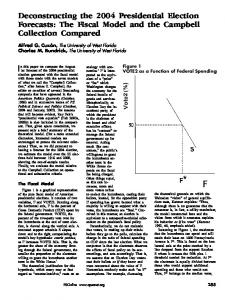
endum on the president's fiscal policy. Parenthetically, we do .... (In 2004, George. W. Bush became the third exception.) ...... original decision to go to war in Iraq.
Feb 16, 2015 - Downloaded by [Julie Nicholson] at 22:45 22 February 2015 .... as play under siege (Zigler & Bishop-Josef, 2004), resulting from a complex ...
spam is a nuisance to users as well as search engines: users .... SEO attempts to boost the PageRank of a web page p by ...... 10th Int. Conf. on DB & Expert.
Raymond, E. S. The Cathedral and the Bazaar, First. Monday, 3(3), 1998. ..... 2Dipartimento di Elettronica per l'Automazione, Università di Brescia, Brescia, Italy.
Characters like Herzog, Joseph or Charles Citrine in Saul Bellow's novels Herzog ... Is Rich (1981) and Rabbit at Rest (1990); Tod Andrews in Barth's The Floating .... genres, such as the picaresque, the epistolary novel or the historical story.
Mar 1, 2004 - A Generalization and Solution to the Common Ancestor Dilemma Problem in .... purpose C++ programming language will be used to write dynamic AOP systems. ..... modified version of the default Java class loader. ...... developers who want
Mar 31, 2005 - proofreading the final manuscripts. Finally, we would like to .... be used to jump to a specified hit anywhere in the file. 5 Word List / Keyword List ...
Mar 1, 2004 - http://java.sun.com/products/jmx/overview.html," Sun Microsystems Inc., 2003. ..... matching the sub-crosscut, one can set a flag when such a join point ...... as the result of the composer's weaving together of a 'tangled web' of.
OFFSET DUPLICATING MACHINE OPERATOR. DISTINGUISHING FEATURES
OF THE CLASS: The work involves the responsibility for the duplication of a ...
(Consigliere della Fondazione Cassa di Risparmi di Livorno), and L. Pesce (Vitrium Galleria, Populonia). Funds made available by Universitá di Pisa (Centro ...
[email protected] ... PDF files can be found at the workshop .... Shadow objects mask one or more methods in a target object (the âshadowedâ object). A.
of the intersections of race, class, gender and culture which operate in the acceptance (or ... counting the number of i
biguous No Man's Land, filled with pits and mines, which may be crossed on a great variety of more or less tortu- ous routes. Once one has indeed crossed this ...
2004 Workshop on Duplicating, Deconstructing and ...
Jun 20, 2004 - Roland E. Wunderlich, Thomas F. Wenisch, Babak Falsafi, and James C. Hoe. Carnegie Mellon ...... [6] J. D. McCalpin, âMemory Bandwidth and.
2004 Workshop on Duplicating, Deconstructing and Debunking June 20, 2004 Munich, Germany Organized by: Bryan Black, Intel Labs, [email protected] Mikko Lipasti, University of Wisconsin, [email protected]
Final Program Session 1: Simulation Methodology Deconstructing and Improving Statistical Simulation in HLS.......2 Robert H. Bell Jr., Lieven Eeckhout, Lizy K. John, and Koen De Bosschere University of Texas at Austin and Ghent University An Evaluation of Stratified Sampling of Microarchitecture Simulations.......13
Roland E. Wunderlich, Thomas F. Wenisch, Babak Falsafi, and James C. Hoe Carnegie Mellon University MicroLib: A Case for the Quantitative Comparison of Micro-Architecture Mechanisms.......19 Daniel Gracia Pérez, Gilles Mouchard, and Olivier Temam
LRI, Paris Sud/11 University and INRIA Futurs, France Session 2: Multiple Threads and Processors The Case of Chaotic Routing Revisited.......32
Cruz Izu, Ramon Beivide and Jose Angel Gregorio University of Adelaide and University of Cantabria Debunking then Duplicating Ultracomputer Performance Claims by Debugging the Combining Switches.......42 Eric Freudenthal and Allan Gottlieb New York University Multiprogramming Performance of the Pentium 4 with Hyper-Threading......53 James R. Bulpin and Ian A. Pratt University of Cambridge
Deconstructing and Improving Statistical Simulation in HLS Robert H. Bell Jr.† †
Lieven Eeckhout ‡
Lizy K. John †
Koen De Bosschere ‡
‡ Department of Electrical and Computer Engineering Department of ELIS The University of Texas at Austin Ghent University, Belgium {belljr, ljohn}@ece.utexas.edu [email protected]
Abstract
model. Since the number of instructions is small and their workload characteristics have been determined by a statistical distribution, the simulation converges to a result much faster than cycleaccurate simulations. The workload statistics include microarchitecture-independent characteristics such as instruction mix and inter-instruction dependency frequencies. They also include microarchitecturedependent statistics such as branch prediction accuracy and cache miss rates for specific branch predictor and cache configurations. These are used to model locality structures dynamically as the simulation proceeds. Statistical simulation systems that correlate well with execution-driven simulators have been shown to exhibit good relative accuracy as microarchitecture changes are applied in design studies [3]. Studies have achieved average errors smaller than 5% on specific benchmark suites [4, 8]. In this study, we quantify the correlation of HLS over a range of benchmarks, from generalpurpose applications to technical and scientific benchmarks, and streaming kernels. In addition to the SPEC95 benchmarks [12], we study singleprecision versions of the STREAM and STREAM2 benchmarks [13]. On these benchmark suites, we find that HLS has an average error of 15.5%. The purpose of this study is to investigate exactly why HLS is not more accurate. Simultaneously we work to improve HLS. We enhance the workload model by collecting information at the basic block level instead of at the instruction level, and we add more detail to the processor model. We find that the overall error decreases from 15.5% to 4.1%, a factor of 3.78. We use the same basic block simulation techniques as in [4], so the error is similar. However, in this study, we start with the HLS framework as a base and in-
Statistical simulation systems can provide an accurate and efficient way to carry out early design studies for processors. One such system, HLS, has a rapid simulation capability, but our experiments demonstrate that several modeling improvements are possible. The front-end graph structure in HLS is hampered by workload modeling at the instruction level that reduces the accuracy of program simulation. The workload and processor models require significant changes to provide accurate results for a variety of benchmarks. We improve HLS by modeling the workload at the granularity of the basic block and by changing the processor model to more closely reflect components in modern microprocessors. The specific techniques improve HLS accuracy by a factor of 3.78 at the cost of increased storage and runtime requirements. Our examination of HLS points to a pitfall for simulator developers: reliance on a single small set of benchmarks to qualify a simulation system. A simple regression model shows that the SPECint95 benchmarks, the original benchmarks used to calibrate HLS, have characteristics that yield to very simple modeling. 1. Introduction To address the extremely long simulation times of modern processor designs, researchers have developed statistical simulation systems [25, 7, 8]. Statistical simulation uses workload statistics from specialized functional or trace-driven simulation to create a synthetic trace that is applied to a fast and flexible execution engine. In HLS [8], statistics are used to create a static control flow graph of a small number of statistically generated instructions. The graph is then walked and the instructions are simulated in a processor
2
crementally add modeling detail to uncover the additional complexity necessary to improve HLS. We quantify the cost of the improvements in terms of additional storage requirements. A simple regression model indicates that CPI results for the SPECint95, the benchmarks originally used to calibrate HLS, can yield to very simple modeling. Our analysis points to a larger problem for simulator developers: using a small set of benchmarks, datasets and simulated instructions to calibrate a simulation system. In the next section, we describe HLS. In Section 3, we describe various modeling problems that we found in HLS. In Section 4, we investigate improvements to the system. We quantify the costs of the improvements in Section 5, followed by conclusions and references.
predecessor is not known. The basic blocks are connected into a graph structure. Each branch has both a taken pointer and a not-taken pointer to other basic blocks. The percentage of backward branches, set statically to 15% in the code, determines whether the taken pointer is a backward branch or a forward branch. For backward or forward branches, a normal random variable over either the mean backward or forward jump distances (set statically to ten and three in the code, respectively) determines the taken target. Later, during simulation, normal random variables over the branch predictability obtained from the sim-outorder run determine dynamically if the branch is actually taken or not, and the corresponding branch target pointer is followed. After the machine statistics are processed and the basic blocks are configured, the instruction graph is walked. As each instruction is encountered, it is simulated on a generalized superscalar execution model for ten thousand cycles. The IPC is averaged over twenty simulations. The generalized model contains fetch, dispatch, execution, completion, and writeback stages. Fetches are buffered up to the fetch width of the machine. Instructions are dispatched to issue queues in front of the execution units and executed as their dependencies are satisfied. Neither an issue width nor a commit width is specified in the processor model. In HLS, the procedure is to first calibrate the generalized processor model using a test workload; then a reference workload is executed on the model. For loads, stores, and branches, the locality statistics determine the necessary delay before issue of dependent instructions. To provide comparison with the SimpleScalar lsq, loads and stores are serviced by a single queue. Parallel cache miss operations are provided through the two memory ports available to the load-store execution unit. As in SimpleScalar, stores execute in zero-time when they reach the tail of their issue queue and the execution unit is available.
2. HLS Overview In the HLS system [8], machine-independent characteristics are analyzed using a modified version of the sim-fast functional simulator from the SimpleScalar release 2.0 toolset [1]. An instruction mix frequency distribution is generated that consists of the percentages of integer, float, load, store and branch instructions. The mean basic block size and standard deviation are also computed. Also generated is the frequency distribution of the dependency distances between instructions for each input of the five instruction types. The benchmarks are executed for one billion cycles in sim-outorder [1]. Sim-outorder provides the IPC used to compare against the IPC obtained in HLS statistical simulation. It also computes the L1 Icache and D-cache miss rates, the unified L2 cache rate, and the branch predictability. After the workload is characterized, HLS generates one hundred basic blocks using a normal random variable over the mean block size and standard deviation. A uniform random variable over the instruction mix distribution fills in the instructions of each basic block. For each randomly generated instruction, a uniform random variable over the dependency distance distribution generates a dependency for each instruction input. An effort is made to make an instruction independent of a store within the current basic block, but if the dependency stretches beyond the limits of the current basic block, no change is made because the dynamic
3. Issues in HLS In this section, we first describe the experimental setup and benchmarks used in our experiments, followed by our examination of HLS, including descriptions of several workload and processor modeling issues.
3
baseline random not-taken single loop
2
1.2 1 0.8 IPC
1.2 0.8
0.6 0.4
0.4
0.9
0.8
0.7
0.6
0.5
0.4
0.3
0.2
0.15
0.1
0.05
0
li
go
com press
vortex
ijpeg
m 88ksim
0.2
perl
Figure 2: IPC vs. Changes in Fraction of Backward Jumps (gcc )
Figure 1: Effect of Graph Connectivity Changes
sequence of basic blocks, with the last basic block pointing back to the first. The maximum error versus the base system is 3.6% for perl using the random not-taken strategy. This is well below the average HLS correlation error versus the SimpleScalar. Figure 2 shows the IPC for gcc as the fraction of backward jumps changes. The hard-coded HLS default is 15% backward jumps. The maximum error versus that default is 2.8%. Figure 3 shows IPC as the backward and forward jump distances are changed from a default of ten and three, respectively. The maximum error versus either of those is 2.0%. From these figures, it is apparent that the graph connectivity in HLS has no impact on simulation performance. Intuitively, HLS models the workload at the granularity of the instruction. All instructions in all basic blocks in the graph are generated identically. The instruction type and dependencies assigned to any slot in any basic block in the graph is randomly selected from the global instruction mix distribution, so the instruction found at any slot on a jump is just as likely to be found at any other slot.
3.1. Experimental Setup and Benchmarks For our experiments we follow the procedure in [8] using the software available at [9]. SimpleScalar and the statistical simulation software were compiled to target big-endian PISA binaries on an IBM Power3 p270. Using the default parameters in [8], sim-outorder was executed on the SPECint95 binaries found at [11] for up to one billion instructions of one reference input dataset, as in [8]. The modified sim-fast was executed on the input dataset for fifty billion instructions, to approximate complete program simulation. In these experiments we use the SPEC CPU 95 integer benchmarks [12] for direct comparison with the original HLS results. We add the SPEC CPU 95 floating point benchmarks [12] and single-precision versions of the STREAM and STREAM2 benchmarks [6, 13]. We include this last suite of benchmarks because they are particularly challenging to statistical simulation systems. In Section 2.5 we discuss the characteristics of the STREAM benchmarks in more detail. 3.2. The HLS Graph Structure We first examine the HLS front-end graph structure. We vary the percentages of backward branches, the backward branch jump distance, the forward branch jump distance, and the graph connections themselves. Figure 1 shows the effect of varying the front-end graph connectivity. Baseline is the base HLS system running with the taken and not-taken branches connected as described in Section 2. Random not-taken is the base system with the nottaken target randomly selected from the configured basic blocks. Single loop is the base system with the taken and not-taken targets of each basic block both pointing to the next basic block in the
backward jump distance
forward jump distance
1.2 1 0.8 IPC
0.6 0.4 0.2
Figure 3: IPC vs. Changes in Backward/Forward Jump Distance (gcc)
4
10
9
8
7
6
5
4
3
2
0 1
0
gcc
IPC
1.6
1B Instructions
dependency fix
50 40 30 20
ssum1
striad
sscale
ssum2
scopy
sfill
sdot
swim
saxpy
fpppp
wave5
apsi
turb3d
applu
m grid
hydro2d
su2cor
li
tom catv
go
compress
vortex
ijpeg
perl
0
m88ksim
10 gcc
IPC Prediction Error (%)
baseline
Figure 4: HLS Error as Modeling Changes
There is also a small probability that the random graph connectivity causes skewed results because the randomly selected taken targets can form a small loop of basic blocks, effectively pruning other parts of the graph from the simulation. This is not a major problem for HLS, in which all blocks are essentially the same, but it has implications for our improvements to HLS described below, so the single loop strategy is employed for the remainder of this paper.
model. Recall that, in standard HLS, measuring microarchitecture-independent characteristics is carried out on the complete benchmark using simfast, whereas microarchitecture-dependent locality metrics are obtained only for the first one billion instructions using sim-outorder. It stands to reason that workload information and locality information should be collected over the same cycle ranges. The 1B Instructions run gives results with sim-fast executing the same one billion instructions as sim-outorder. Not all benchmarks improve, but the error in SPECfp95 drops by half from 13.6% to 6.8%. Overall error decreases from 15.5% to 13.1%. The modified sim-fast makes no distinction between memory instructions that carry out autoincrement or auto-decrement on the address register after memory access and those that do not. The HLS sim-fast code always assumes the modes are active. This causes the code to assume register dependencies that do not actually exist between memory access instructions, and it makes codes with significant numbers of load and store address dependency fix
STREAM
All
30 25 20 15 10 5 0
1B Instructions
SPECfp
baseline IPC Prediction Error (%)
3.4. Modeling Workload Characteristics Figures 4 and 5 show the IPC prediction error [4] over all benchmarks as workload modeling issues are incrementally addressed. The baseline run gives the HLS results out-of-thebox. While SPECint95 does well as in [8] with only 5.8% error, SPECfp95 has twice the correlation error. The STREAM loop error is more than four times worse at 27%. We were unable to achieve accurate results on all the benchmarks by recalibrating the generalized HLS processor
SPECint
3.3. The HLS Processor Model In the HLS generalized execution model, there is no issue-width concept. The issue of instructions to the issue queues is instead limited by the queue size and dispatch window and, ultimately, by the fetch window. There is also no specific completion width in HLS, so the instruction completion rate is also front-end limited. These omissions are conducive to obtaining quick convergence to an average result for well-behaved benchmarks, but they make it difficult to correlate the system to SimpleScalar for a variety of benchmarks.
Figure 5: Overall HLS Error as Modeling Improves
5
3.5.
Loop Challenges Table 2 shows single-precision versions of the STREAM benchmarks, including the loop equation and the number of instructions in the kernel loop when compiled with gcc using -O. The STREAM loops are strongly phased, and in fact have only a single phase. Loops consist of one or a small number of tight iterations containing specific instruction sequences that are difficult for statistical simulation systems to model. Figure 6 shows one iteration of the saxpy loop (in the PISA language [1]). If the mul.s and add.s were switched in the random instruction generation process leaving the dependency relationships the same, the extra latency of the multi-cycle mul.s instruction is no longer hidden by the latency of the second l.s, leading to a generally longer execution time for the loop. A similar effect can be caused by changes in dependency relationships as the dependencies are statistically generated from a distribution. Shorter runs can also occur. The mul.s has a dependency on the previous l.s. If the l.s is switched with the one-cycle add.s, keeping dependencies the same, the mul.s can dispatch much faster. While higher-order ILP distributions might work well for some loops, the results have been mixed and can actually lead to decreased accuracy for general-purpose programs [3].
Table 1: CPI Regression Analysis over 1B Instructions Benchmarks
2
Targeted CPI
R
HLS
0.988
SimpleScalar
0.970
SPECint
HLS
0.972
SimpleScalar
0.895
SPECint and SPECfp
HLS
0.757
SimpleScalar
0.811
SPECint, SPECfp and STREAM
register dependencies, including the STREAM loops, appear to run slower. The sim-fast code was modified to check the instruction operand for the condition and mark dependencies accordingly, and the dependency fix bars in the figures give the results. The STREAM loops are improved, but the SPECint95 error increases from 4.8% to 9.3%. This is most likely due to the original calibration of the generalized HLS processor model in the presence of the modeling error. Table 1 shows a simple regression analysis over the locality features taken from sim-outorder runs: branch mispredictability, L1 I-cache and Dcache miss rates, and L2 miss rate. The targeted CPI is the particular CPI targeted in the analysis, either SimpleScalar or the HLS result. The squared correlation coefficient, R2, is a measure of the variability in the CPI that is predictable from the four features. The SPECint95 benchmarks always achieve high correlation, while the analysis over all benchmarks or even over SPECint95 together with SPECfp95 achieve lower correlation. This is an indication that a very simple processor model can potentially represent the CPI of the SPECint95 by emphasizing the performance of the locality features; but it can not as easily do the same over all three suites.
4. Improving HLS In this section, we focus on improving the processor and workload models to give more accurate simulation results. 4.1. Processor Model It is difficult to correlate the generalized HLS processor model to SimpleScalar for all benchmarks. For this reason, we augmented HLS with a register-update-unit (RUU), an issue width
and a completion width. We also rewrote the recurrent completion function to be non-recurrent and callable prior to execution, and we rewrote the execution unit to issue new instructions only after prior executing instructions have been serviced in the current cycle. We added code to differentiate long and short running integer and floating point instructions. To maintain efficiency, the locality structures are still modeled using the statistical parameters taken from simoutorder runs. We first run the benchmarks on the improved processor model using the same workload characteristics modeled in HLS, except that we generate one thousand basic blocks instead of one hundred, and we simulate for twenty thousand cycles in stead of ten thousand; so simulation time is about twice that in HLS. (The same changes in HLS do not decrease error.) The execution engine flow, delays and parameters are all chosen to match those in the SimpleScalar default configuration. The baseline system was validated by comparing sim-outorder traces, obtained from sections of the STREAM loops, to traces taken from the improved HLS assuming perfect caches and perfect branch predictability. The validation was simplified by the fact that the loops are comprised of only one phase. Figure 7 gives the results for the individual benchmarks, and Figure 8 shows the average results per benchmark suite. The baseline run gives the improved system results using the default SimpleScalar parameters and using the global instruction mix, dependency information, and
load and store miss rates. There are errors greater than 25% for particular benchmarks, such as ijpeg, compress and apsi. The overall error of 14.4% compares well with the 15.5% baseline error in HLS, but it is higher than the 13.1% error in shown in Figure 5 for HLS with improved workload modeling. 4.2. Workload Model We also enhanced the workload model to reduce correlation errors. The analysis of the graph structure showed that modeling at the granularity of the instruction in HLS did not contribute to accuracy. In [7], the basic block size is the granule of simulation. However, this raises the possibility of basic block size aliasing, in which many blocks of the same size but very different instruction sequences and dependency relationships are combined. sequences bpred
dependencies stream info
20 15 10
STREAM
SPECfp
0
SPECint
5 All
IPC Prediction Error (%)
baseline miss rates
Figure 8: Improved HLS Average Error as Modeling Changes
7
4.2.1. Basic Block Modeling Granularity Instead of risking reduced accuracy with block size aliasing, we model at the granularity of the basic block itself. The dynamic frequencies of all basic blocks are used as a probability distribution function for building the sequence of basic blocks in the graph. This is the same as the k=0 modeling in the SMART-HLS system [4]. To capture cache and branch predictor statistics for the basic blocks, we use sim-cache augmented with the sim-bpred code. In the sequences bars of Figures 7 and 8, the basic block instruction sequences are used, but the dependencies and locality statistics for each instruction in each basic block are still taken from the global statistics found for the entire benchmark. The overall correlation errors are reduced dramatically for the three classes of benchmarks. However, some benchmarks such as compress and hydro2d, and the STREAM loops, still show high correlation errors. In the dependencies run, we include the use of dependency information for each basic block. In order to reduce the amount of information stored, we merge the dependencies into the smallest dependency relationship found in any basic block with the same instruction sequence, as in [4]. The average error is reduced significantly from 8.9% to 6.3%. On investigation, it was found that the global miss rate calculations do not correspond to the miss rates from the viewpoint of the memory operations in a basic block. In the cache statistics, HLS pulls in the overall cache miss rate number from SimpleScalar, which includes writebacks to the L2. But for individual memory operations in a basic block, the part of the L2 miss rate due to writebacks should not be included in the miss rate. This is because the writebacks generally occur in parallel with the servicing of the miss so they do not contribute to the latency of the operation. This argues for either a global L2 miss rate calculation that does not include writebacks or the maintenance of miss rate information for each basic block. In addition, examination of the STREAM loops reveals that the miss rates for loads and stores are quite different. In saxpy, for example, both loads miss to the L1, but the store always hits. Because of these considerations, the L1 and L2 probabilistic miss rates for both loads
and stores should be maintained local to each basic block. The miss rates run includes this information. All benchmarks improve, but a few of the STREAM loops still have errors greater than 10%. The problem is that the STREAM loops need information concerning how the load and store misses, or delayed hits, overlap. In most cases load misses overlap, but the random cache miss variables often cause them not to overlap, leading to an underestimation of performance. Note that this is the reverse of the usual situation for statistical simulation in which critical paths are randomized to less critical paths, and performance is overestimated. An additional run, bpred, includes branch predictability local to each basic block. This helps a few benchmarks like ijpeg and hydro2d, but, as expected, the STREAM loops are unaffected. One solution is to keep overlap statistics. This solves the delayed hits problem, but does not provide for the modeling of additional memory operation features. Instead, when the workload is characterized, we track one hundred L1 and L2 hit/miss indicators (i.e. if the memory operation was an L1 hit or miss or an L2 hit or miss) for the sequence of loads and stores in each basic block near the end of the one billion instruction simulation. Later, during statistical simulation, we use the stream indicators in order (but without pairing them to particular memory operations) to determine the miss characteristics of the stream as the loads and stores are encountered. This is a simplistic way to operate, since the stream hit/miss indicators are simply collected at the end of the run and are therefore not necessarily representative of the entire run. However, the technique may be applicable given the trend to identify and simulate program phases [10] in which stream information may change little. Still, simulating one billion instructions without regard to phase behavior, we expect the technique to help only the STREAM loops, and to negatively affect the others. The stream info bars in Figure 7 show the results. As expected, the STREAM loops improve significantly. However, only a small amount of accuracy is lost for the others. This indicates that there is only one or a small number of phases in the first one billion instructions for most bench-
8
ssum 1
striad
sscale
ssum 2
scopy
sfill
sdot
stream info
saxpy
swim
bpred
fpppp
apsi
wave5
miss rates
turb3d
applu
m grid
hydro2d
dependencies
su2cor
tom catv
li
go
sequences
com pres
vortex
ijpeg
m 88ksim
perl
45 40 35 30 25 20 15 10 5 0 gcc
IPC Prediction Error (%)
baseline
Figure 9: Improved HLS Error as Modeling Changes Using Basic Block Maps
marks, at least with respect to the load and store stream behavior.
trol flow graph of the program. A system to do that for the SPEC2000 benchmarks is presented in [4]. Since the phase identification is carried out continuously during simulation, the possibility exists of not only detecting the coarse-grained phases, but also the micro-phases, or small shifts in relative block frequencies, that must be identified in order to achieve good accuracy using statistical simulation. Following [4], we annotate each basic block with a list of pointers to its successor blocks along with the probabilities of accessing each successor. By walking the basic blocks as in the previous section, but using a random variable over the successor probabilities to pick the successor, the program phase behavior is uncovered. We simulate all strategies as before. Figures 9 and 10 show the basic block map results. The overall error using all techniques is improved only a little from 4.35% to 4.11%, a sequences bpred
dependencies stream info
20 15 10
STREAM
0
SPECfp
5 All
IPC Prediction Error (%)
baseline miss rates
SPECint
4.2.2. Basic Block Maps In the previous simulations, the basic blocks were not associated with each other in any way since a random variable over the frequency distribution of the blocks is used to pick the next basic block to be simulated. At branch execution time, a random variable based on the global branch predictability is used simply to indicate that a branch misprediction occurred when the branch was dispatched, causing additional delay penalty before the next instruction can be fetched, but that is not related to the successor block decision. This technique treats all blocks together as if no phases exist in which one area of the graph is favored over another at different times. By associating particular basic blocks with each other in specific time intervals, for example during a program phase, it is expected that better simulation accuracy can be obtained for multiphase programs. One way to do that is to specify the phases, the basic blocks executing in those phases, and the relative frequencies of the basic block executions during those phases. These three things together constitute a basic block map. The phase identification requires knowledge of when the relative frequencies of the basic blocks change. The identification of phases at a coarse granularity can be carried out using a phase identification program such as SimPoint [10]. It can also be developed dynamically during simulation by walking a representation of the con-
Figure 10: Improved HLS Average Error as Modeling Changes Using Basic Block Maps
9
HLS
0 ssu sco avg ssc ssu sd sdo ot ale m2 py_ m2 t_s _ss sum _sfill _ _s s s do do fill um t 1 t 2
Figure 12: HLS vs. Improved HLS with Basic Block Maps
Figure 11: HLS and Improved HLS on Two-Phase Benchmarks
5.5% decrease. SPECint95 is improved from 6.9% to 4.3%, or 38% on average. The STREAM loops are unchanged since they consist of a single phase, and there is no advantage in using basic block maps in that case. The SPECfp95 show an increase in error from 3.3% to 4.7%. Part of this is due to the negative effects of using stream information, which cause a jump up from 3.6% error for SPECfp95. The low overall improvement agrees with the results found in the last subsection, in which stream information, which should be phase dependent, causes little adverse reaction. Coupled with increased variance by simulating only twenty thousand cycles, the result is not surprising. Improvements are also limited by errors in the graph structure, including the merge of dependencies explained earlier. Basic block maps demonstrate improvement on programs with a number of strong phases. To demonstrate the effectiveness of the technique, several benchmarks are created using combinaHLS
SPECfp
10
SPECint
20
All
30
30 25 20 15 10 5 0
Improved HLS
STREAM
Improved HLS (bbmaps) IPC Prediction Error (%)
Improved HLS
40
tions of the STREAM loops. Figure 11 shows, for example, that a simple code created from the concatenation of sdot and ssum1 has correlation errors of 39.4% and 14.8% in HLS and the improved HLS without basic block maps, respectively. In the improved HLS without basic block maps, given that 50% of the blocks are equivalent to sdot blocks, and 50% are equivalent to ssum1 blocks, the resulting sequence of basic blocks is a jumble of both. The behavior of the resulting simulations tends to be pessimistic with longlatency L2 cache misses forming a critical chain in the dispatch window. When the basic block map technique is applied, the error shrinks to 0.4% because the sequence of simulated basic blocks is more accurate. Figure 12 and 13 compare HLS to HLS with basic block maps running with all optimizations. The improvements show a 4.1% average error, which is 3.78 times more accurate than the original HLS at 15.5% error. Improved HLS
50 40 30 20
Figure 13: HLS vs. Improved HLS with Basic Block Maps
10
ssum1
striad
sscale
ssum2
scopy
sfill
sdot
saxpy
swim
fpppp
wave5
apsi
applu
turb3d
m grid
hydro2d
su2cor
tomcatv
li
go
vortex
compres
ijpeg
gcc
0
m88ksim
10 perl
IPC Prediction Error (%)
IPC Prediction Error (%)
HLS
5. Implementation Costs Table 3 shows the cost of the improvements in bytes as a function of the number of basic blocks (NBB), the average length of the basic blocks (LBB), the average number of loads and stores in the basic block (NLS), the average number of successors in the basic blocks (SBB), and the amount of stream data used (NSD). NSD is NLS x 100 = 4.71 x 100 = 471 in our runs. Table 4 shows the error reduction as the average reduction in correlation error as each technique augments the previous technique. There are only five instruction types, so we use four bits to represent each. There are two dependencies per instruction, each of which is limited to within 255; so two bytes of storage per instruction are needed. We maintain both load and store miss rates for the L1 and L2 caches; so four floats are needed. For basic block maps, the successor pointer and frequency are maintained in in a 32-bit address and a float. Clearly, including detailed stream data is inefficient on average compared to using the other techniques, but future work, including phase identification techniques, can seek to reduce the amount of data being collected.
Table 3: Benchmark Information Number Average Average Average Name of basic Block Ld St per Number of Block Successors blocks Length gcc 2714 12.74 6.07 2.19 perl
6. Conclusions Statistical simulation can provide an accurate and efficient simulation capability. In the HLS system, we identified several issues related to workload and processor modeling that affect simulation accuracy negatively. One workload modeling issue is that the front-end graph structure of HLS operates at the
575
9.39
4.93
1.82
m88ksim
398
10.90
4.7
1.86
ijpeg
661
13.09
6.03
1.76
vortex
1134
14.38
8.53
1.64
compress
151
8.30
3.4
1.94
go
1732
15.17
5.01
2.26
li
318
8.74
4.42
1.96
tomcatv
258
8.91
3.9
1.9
su2cor
406
9.58
3.84
1.76
hydro2d
646
11.91
3.99
1.81
mgrid
450
12.41
4.74
2.02
applu
552
25.24
8.21
1.87
turb3d
496
12.57
4.92
1.77
apsi
1010
17.94
8.45
1.65
wave5
507
9.89
3.96
1.86
fpppp
452
18.94
8.59
1.77
swim
419
12.44
4.66
1.91
saxpy
177
9.01
3.55
2.12
sdot
109
8.58
3.92
2.3
sfill
177
8.94
3.53
2.12
scopy
177
8.97
3.54
2.12
ssum2
109
8.50
3.89
2.3
sscale
177
8.98
3.54
2.12
striad
177
9.03
3.55
2.12
ssum1
177
9.02
3.55
2.12
Average
524.4
10.7
4.71
1.89
Table 4: Implementation Costs Technique Cumulative Frequencies Sequences Dependencies Miss Rates Branch Predictability Stream Info Basic Block Maps Overall
Cost Formula (Bytes)
Avg. Cost Per Benchmark (Bytes)
Percent Error Reduction
Cost Per Percent Error Reduction (Bytes)
42.7%
115
~Storage per Block
NBB x 4
2098
1 Float
NBB x LBB x ½
2806
NBB x LBB x 2 x 1
11222
25.4%
442
22 Bytes
NBB x 4 x 4
4195
6.5%
645
4 Floats
NBB x 4
2098
2.3%
912
1 Float
NBB x NSD x ¼
61701
25.0%
2468
118 Bytes
NBB x SBB x 2 x 4
7929
5.3%
1496
4 Floats
92049
73.5%
1252
186 Bytes
6 Bytes
11
granularity of the instruction and contributes little to the performance of the system. The HLS processor model does not implement a specific issue width or a commit width, making calibration to a detailed processor simulator such as SimpleScalar difficult. To meet these challenges, we model the workload at the granularity of the basic block and recode the processor model to decrease error. We find that IPC prediction error can be reduced from 15.5% to 4.1%. We quantify the cost of the improvements in terms of increased storage requirements and find that less than 100K bytes on average are needed per benchmark to achieve the maximum error reduction. Runtime is approximately twice that of HLS. A simple regression analysis shows that the SPECint95 workload is susceptible to very simple processor models. Our results point to a major pitfall for simulator developers: reliance on a small set of benchmarks, datasets and simulated instructions to qualify a simulation system.
IEEE Micro, Vol. 23 No. 5, Sept/Oct 2003, pp. 26-38. [4] L. Eeckhout, R. H. Bell Jr., B. Stougie, K. De Bosschere and L. K. John, “Improved Control Flow in Statistical Simulation for Accurate and Efficient Processor Design Studies,” Proceedings of the International Symposium on Computer Architecture, June 2004, to appear. [5] C. P. Joshi, A. Kumar and M. Balakrishnan, "A New Performance Evaluation Approach for System Level Design Space Exploration," IEEE International Symposium on System Synthesis, October 2002, pp. 180-185. [6] J. D. McCalpin, “ Memory Bandwidth and Machine Balance in Current High Performance Computers,” IEEE Technical Committee on Computer Architecture Newsletter, December 1995. [7] S. Nussbaum and J. E. Smith, "Modeling Superscalar Processors Via Statistical Simulation," Proceedings of the International Conference on Parallel Architectures and Compilation Techniques, September 2001, pp. 15-24.
Aknowledgements The authors would like to thank the anonymous reviewers for their feedback. Rob Bell is supported by the IBM Graduate Work Study program and the Server and Technology Division of IBM. Lieven Eeckhout is a Postdoctoral Fellow of the Fund for Scientific Research – Flanders (Belgium) (F.W.O. Vlaanderen). This research is also partially supported by the Institute for the Promotion of Innovation by Science and Technology in Flanders (IWT), by Ghent University, by the United States National Science Foundation under grant number 0113105, and by IBM, Intel and AMD corporations.
[8] M. Oskin, F.T.Chong and M. Farrens, "HLS: Combining Statistical and Symbolic Simulation to Guide Microprocessor Design," Proceedings of the 27th Annual International Symposium on Computer Architecture, June 2000, pp. 71-82. [9]http://www.cs.washington.edu/homes/okskin/t ools.html [10] T. Sherwood, E. Perelman, G. Hamerly and B. Calder, “ Automatically Characterizing Large Scale Program Behavior,” Proceedings of the International Conference on Architected Support for Programming Languages and Operating Systems, October 2002, pp. 45-57.
References [1] D. C. Burger and T. M. Austin, “The SimpleScalar Toolset,” Computer Architecture News, 1997.
[2] R. Carl and J. E. Smith, "Modeling Superscalar Processors Via Statistical Simulation,” Workshop on Performance Analysis and Its Impact on Design, June 1998.
[13]http://www.cs.virginia.edu/stream/ref.html
[3] L. Eeckhout, S. Nussbaum, J. E. Smith and K. De Bosschere, “ Statistical Simulation: Adding Efficiency to the Computer Designer’s Toolbox,”
12
An Evaluation of Stratified Sampling of Microarchitecture Simulations Roland E. Wunderlich Thomas F. Wenisch Babak Falsafi James C. Hoe Computer Architecture Laboratory (CALCM) Carnegie Mellon University, Pittsburgh, PA 15213-3890 {rolandw, twenisch, babak, jhoe}@ece.cmu.edu http://www.ece.cmu.edu/~simflex
Abstract
growing—with as much as five orders of magnitude slowdown currently. Thus, researchers have begun looking for ways to accelerate simulation without sacrificing the accuracy and reliability of results [1,5,6,7]. One of the most promising approaches to accelerate simulation is to evaluate only a tiny sample of each workload. Previous research has demonstrated highly accurate results while reducing simulation run time from weeks to hours [6,7]. These sampling proposals pursue two different approaches to sample selection: (1) statistical uniform sampling of a benchmark’s instruction stream, and (2) targeted sampling of non-repetitive benchmark behaviors. Uniform sampling, such as the SMARTS framework [7], has the advantage that it requires no foreknowledge or analysis of benchmark applications, and it provides a statistical measure of the reliability of each experimental result. However, this approach ignores the vast amount of repetition within most benchmark’s instruction streams, taking many redundant measurements. Targeted sampling instead categorizes program behaviors to select fewer measurements, reducing redundant measurements. The SimPoint approach [6] identifies repetitive behaviors by summarizing fixed-size regions of the dynamic instruction stream as basic block vectors (BBV), building clusters of regions with similar vectors, and taking one measurement within each cluster. The benefits of both sampling approaches can be achieved by placing the phase identification techniques of targeted sampling in a statistical framework that provides a confidence estimate with each experiment. Stratified random sampling is this statistical framework. Stratified sampling breaks a population into strata, analogous to targeted sampling, and then randomly samples within each stratum, as in uniform sampling. By separating the distinct behaviors of a benchmark into different strata, each behavior can be characterized by a small number of measurements. Each of these characterizations is then weighted by the size of the stratum to compute an overall estimate. The aggregate number of measurements can be lower than the number required by uniform sampling. The effectiveness of stratified sampling can be evaluated along two dimensions. First, it might reduce the total
Recent research advocates applying sampling to accelerate microarchitecture simulation. Simple random sampling offers accurate performance estimates (with a high quantifiable confidence) by taking a large number (e.g., 10,000) of short performance measurements over the full length of a benchmark. Simple random sampling does not exploit the often repetitive behaviors of benchmarks, collecting many redundant measurements. By identifying repetitive behaviors, we can apply stratified random sampling to achieve the same confidence as simple random sampling with far fewer measurements. Our oracle limit study of optimal stratified sampling of SPEC CPU2000 benchmarks demonstrates an opportunity to reduce required measurement by 43x over simple random sampling. Using our oracle results as a basis for comparison, we evaluate two practical approaches for selecting strata, program phase detection and IPC profiling. Program phase detection is attractive because it is microarchitecture independent, while IPC profiling directly minimizes stratum variance, therefore minimizing sample size. Unfortunately, our results indicate that: (1) program phase stratification falls far short of optimal opportunity, (2) IPC profiling requires expensive microarchitecturespecific analysis, and (3) both methods require large sampling unit sizes to make strata selection feasible, offsetting their reductions of sample size. We conclude that, without better stratification approaches, stratified sampling does not provide a clear advantage over simple random sampling.
1. Introduction One of the primary design tools in microarchitecture research is software simulation of benchmark applications. Timing-accurate simulation’s flexibility and accuracy makes it indispensable to microarchitecture research. However, the applications we wish study continue to increase in length—hundreds of billions of instructions for SPEC CPU2000 (SPEC2K). At the same time, the speed gap between simulators and the simulated hardware is
13
Step 1 Benchmark profile
Stratify instruction stream
Step 2 Random sampling of individual strata
Strata membership
We examined optimal, program phase detection, and IPC profiling stratification.
Strata-specific estimates
Step 3 Aggregate estimates & calc. confidence
Optimal sample sizes determined by (3)
(1,2) Benchmark estimates
Figure 1. The stratified random sampling process. We focus on the relative effectiveness of two practical stratification approaches for Step 1 in this work. The referenced equations for Steps 2 & 3 are in Section 2.
The remainder of this paper is organized as follows. Section 2 presents stratified random sampling theory and details how to correctly achieve confidence in results from a stratified population. Section 3 discusses our optimal stratification study, while Section 4 covers our evaluations of two practical stratification techniques. In Sections 3 and 4, we explicitly cover the improvements to sample size and total measured instructions as compared to simple random sampling for each technique. We conclude in Section 5.
quantity of measurements required. For simulators where a large number of measurements implies significant cost— for example, the storage of large architectural state checkpoints to launch each measurement—a reduction of measurements would imply cost savings. More commonly, however, the total number of instructions measured has the larger impact on simulation cost. To improve total measurement, a stratification approach must reduce the quantity of required measurements while maintaining the small measurement sizes achievable with simple random sampling. In this study, we evaluate the practical merit of combining sample targeting with statistical sampling in the form of stratified random sampling. We perform an oracle limit study to establish bounds on improvement from stratification and evaluate two practical stratification approaches: program phase detection and IPC profiling. We evaluate both approaches quantitatively in terms of sample size (measurement quantity) and sampling unit size (measurement size), and qualitatively in terms of the upfront cost of creating a stratification. We demonstrate:
2. Stratified random sampling The confidence in results of a simple random sample is directly proportional to the sample size and the variance of the property being measured. The sample size is the number of measurements taken to make up a sample, and variance is the square of standard deviation. Significant reductions in sample size can often be achieved when a population can be split into segments of lower variance than the whole. Stratified random sampling of a population is performed by taking simple random samples of strata, mutually exclusive segments of the population, and aggregating the resulting estimates to produce estimates applicable to the entire population. Strata do not need to consist of contiguous segments of the population, rather every population member is independently assigned to a stratum by some selection criteria. If stratifying the population results in strata with relatively low variance, a small sample can measure each stratum to a desired confidence. By combining the measurements of individual strata, we can compute an overall estimate and confidence. With low variance strata, the aggregate size of a stratified sample can be much smaller than a simple random sample with equivalent confidence. A population whose distinct behaviors are assigned to separate strata will see the largest decreases in sample size when using stratified sampling. The process of stratified random sampling is illustrated in Figure 1. The first of three steps is to stratify the population into K strata. We discuss various techniques for stratifying populations in the context of microarchitecture simulation in Sections 3 and 4. Second, we collect a simple random sample of each stratum. We represent the variable of interest as x, and strata-specific variables with the subscript h, where h ranges from 1 to K. Therefore, Nh
• Limited gains in sample size: We show that stratifying via program phase detection achieves only a small reduction in sample size over uniform sampling, 2.2x, in comparison to the oracle opportunity of 43x. Phase detection assures that each stratum has a homogenous instruction footprint. Unfortunately, data effects and other sources of performance variation remain. The reduction in CPI variability achieved by stratifying on instruction footprint is not sufficient to approach the full opportunity of stratification. • Expensive analysis and limited applicability: We show that IPC profiling requires an expensive analysis that is microarchitecture specific, and its gains do not justify this cost. • No improvement in total measurement: We show that neither stratification approach improves over simple random sampling in terms of total instructions measured. Because of the computational complexity of clustering, neither stratification approach can be applied at the lowest sampling unit sizes achievable with random sampling. This increase in sampling unit size offsets reductions in sample size for stratified sampling.
• For each K, strata are partitioned using k-means clustering • Minimum strata sample size of 30 is best for reliable confidence estimates due to central limit theorem
3. Sample each stratum individually, aggregate estimates Stratum 1
• Optimal number of strata, K, determined by incrementing K until total stratified sample size is minimized
Stratum 3
Figure 2. Determining the optimal stratification for a particular benchmark and microarchitecture. Collecting the IPC profile requires performance simulation of the full length of the target benchmark.
3. Optimal stratification
is the population size of stratum h, nh is the sample size for stratum h, while V hx is that stratum’s standard deviation of x. The final step is to aggregate the individual stratum estimates to produce estimates of the entire population. A simple weighted mean is used to produce a population mean estimate:
In order to evaluate practical stratification approaches for the experimental procedure presented in Section 2, we first quantify the upper bound reduction in sample size achievable with an optimal stratification. As in previous studies of simulation sampling [7, 6], we focus on CPI as the target metric for our estimation, and use the same 8way and 16-way out-of-order superscalar processor configurations, SPEC2K benchmarks, and simulator codebase as [7]. Determining an optimal stratification for CPI requires knowledge of the CPI distribution for the full length of an application—knowledge which obviates the need to estimate CPI via sampling. To perform this study, we have recorded complete traces of the per-unit IPC (not CPI, for reasons explained later) of every benchmark on both configurations. While not a practically applicable technique, this study establishes the bounds within which all practical stratification methods will fall. At worst, an arbitrary stratification approach will match simple random sampling, as random assignment of sampling units to strata is equivalent to simple random sampling. At best, any approach will match the bound established here. Optimal stratified sampling. To minimize total sample size, we need to determine an optimal number of strata, and minimize their respective variances. Then, we calculate the correct sample size for a desired confidence using the optimal stratified sample allocation equation (3). This equation provides the best sample size for each stratum, given their variances and relative sizes. Larger and higher variance strata receive proportionally larger samples. We constrain sample size for each stratum to a minimum of 30 (or the entire stratum, if it contains fewer than 30 elements) to ensure that the central limit theorem holds, and that our confidence calculations are valid [2]. The optimal number of strata, K, cannot be determined in closed form. Intuitively, more strata allows finer classification of application behavior, reducing variance within each stratum, and therefore reducing sample size. However, at some critical K, the floor of 30 measurements
10K 100K 1M 10M 100M U Sam pling Unit Size (Instructions)
Figure 4. Total measured instructions per benchmark with optimal stratification.
Impact on sample size. Figure 3 illustrates the impact of stratification on sample size, n, for the 8-way configuration. The top line in the figure represents the average sample size required for a simple random sample to achieve 99.7% confidence of ±3% error across all benchmarks. The bottom line depicts the average sample size with optimal stratification. Stratification can provide a 43x improvement in sample size for U = 1000 instructions, reducing average sample size from ~8000 to 185 measurements per benchmark. This result demonstrates that random sampling takes many redundant measurements, and that there is significant opportunity for improvement with an effective stratification technique. Impact on total measured instructions. Figure 4 illustrates the impact of stratification on total measured instructions, n · U. The dashed line illustrates the total instructions required for the SMARTS technique, which performs systematic sampling at U = 1000 instructions. The graph shows that any practical stratification approach must be applied at a unit size of 10,000 instructions or smaller in order to have a possibility of outperforming existing sampling methodology.
per stratum dominates and increasing K increases sample size. For each combination of benchmark, microarchitecture, and sampling unit size, U, we determine the total stratified sample size for each value of K up to the optimal value, by starting with K = 1 and stopping when total sample size decreases to a minimum. For each value of K, we determine the optimal assignment of sampling units to strata such that the CPI variance of each stratum is minimized. We employ the k-means clustering algorithm, using the implementation described in [3] that utilizes kd-trees and blacklisting optimizations. The k-means algorithm is one of the fastest clustering algorithms, and the implementation in [3] is optimized for clustering large data sets, up to approximately 1 million elements. (Beyond 1 million elements, the memory and computation requirements render the approach infeasible.) Each k-means clustering was performed with 50 random seeds to ensure an optimal clustering result. To stratify the large populations of SPEC2K benchmarks at small U (on average 174 million sampling units per benchmark at U = 1000 instructions), we must reduce the data set before clustering. Figure 2 illustrates how we reduce the data set without impacting clustering results. We assign sampling units to bins of size 0.001 IPC, and then cluster the bins using their center and membership count. We bin based on IPC rather than CPI as IPC varies over a finite range for a particular microarchitecture (i.e., 0 to 8 for our 8-way configuration, thus, 8000 bins). As long as the number of bins is much larger than K, and the variance within a bin is negligible relative to overall variance, binning does not adversely affect the results of the clustering algorithm. After each clustering, we calculate the variance of the resulting strata and determine an optimal sample size as previously described. We iterate until the critical value for K is encountered. The optimal K lies between one and ten clusters for all benchmarks and configurations that we studied, and tends to decrease slightly with increasing U. Note that the optimal K is independent of the target confidence interval.
4. Practical stratification approaches The optimal stratification study presented in Section 3 establishes upper and lower bounds by which we can measure the effectiveness of any stratification approach. However, creating the optimal stratification requires knowledge of the CPI distribution for the full length of an application, and is optimal only for that specific microarchitecture configuration. In order for stratification to be useful, we must balance the cost of producing a stratification with the time saved relative to simple random sampling over the set of experiments which can use the stratification. Thus, we desire stratifications that can be computed cheaply and can be applied across a wide range of microarchitecture configurations. In the following subsections, we analyze two promising stratification
16
approaches. However, we find that both approaches obtain insufficient execution time improvements over simple random sampling to justify their large costs.
Simple Random Sampling BBV Stratification Optimal Stratification
n Sample Size
10,000
4.1. Program phase detection SimPoint [6] presents program phase detection as a promising approach for identifying and exploiting repetitive behavior in benchmarks to enable acceleration of microarchitecture simulation. SimPoint identifies program phases based upon a basic-block vector profile. SimPoint clusters measurement units based on the similarity of portions of the BBV profiles. Statistically Valid SimPoint [4] presents a method for evaluating the statistical confidence of SimPoint simulations where only a single unit is measured from each cluster. However, the proposed use of parametric bootstrapping only provides confidence interval estimates for the specific microarchitecture where the bootstrap is performed, and does not account for individual experiment’s variations in performance. In addition, this analysis requires CPI data for many points within each cluster. Instead, by applying BBV phase detection in the context of stratified random sampling, we can obtain a confidence estimate with every experiment. By measuring at least 30 units from each stratum (BBV cluster), we satisfy the conditions of the central limit theorem and obtain a confidence estimate with each simulation experiment. The number of strata was optimally selected using the same technique as our optimal stratification study in Section 3. SimPoint seems a promising approach for stratification, as it achieves both of the goals outlined earlier. First, basic block vector analysis is relatively low cost, as it can be accomplished using a BBV trace obtained by functional simulation or direct execution of instrumented binaries (if experimenting with an implemented ISA). Second, basic block vectors are independent of microarchitecture, and thus, the resulting stratification can be applied across many experiments. Practical costs. The primary costs of program phase stratification are the collection of a benchmark’s raw BBV data and the clustering analysis time. Collection of BBV data can be done with direct execution for existing instruction set architectures, otherwise functional simulation is required. For the unit sizes advocated in [4] and [6] of 1 million to 100 million instructions, analysis time for clustering is a few hours at most. However, clustering quickly becomes intractable as we reduce U further. It is infeasible to compute a k-means clustering for U < 100,000, since, for most SPEC2K benchmarks, this results in more than 1 million sampling units. The high dimensionality (15 dimensions after random linear projection) of BBV data prevents the binning optimization done for the optimal stratification study in Section 3 due to the sparseness of the vector space.
1,000
100
10 1M 10M U Sam pling Unit Size (Instructions)
Figure 5. BBV program phase stratification average sample size with the 8-way microarchitecture. BBV stratification reduces average sample size by 2.2x over simple random sampling, but it requires U > 100,000.
Impact on sample size. Program phase detection does provide a modest improvement in sample size over simple random sampling. However, phase detection falls short of optimal stratification since it seeks to ensure the homogeneity of the instruction footprint of each stratum. This does not necessarily lead to minimal CPI variance within each stratum. On average, program phase clustering improves sample size by only 2.2x over simple random sampling as shown in Figure 5. The average sample size at U = 1 million instructions was 3590 for simple random sampling and 1615 for BBV stratified random sampling, as compared to 125 for optimal stratified sampling. Impact on total measured instructions. Because the BBV clustering analysis cannot be performed for U below 100,000, stratification based on program phase cannot match the total measured instructions achievable with simple random sampling. With U = 1 million, BBV stratification results in an average of 1.6 billion instructions measured per benchmark, while a simple random sample with U = 1000 requires only 8 million instructions per benchmark to be measured.
4.2. IPC profiling The optimal stratification study in Section 3 achieves large gains with stratification by stratifying directly on the target metric, in this case CPI. Optimal stratification can not be done for each experiment in practice because it requires the very same detailed simulation that we are trying to accelerate. However, if it were possible to perform this expensive stratification once per benchmark on a test microarchitecture, and then apply this stratification to many other microarchitecture configurations over many experiments, the long term savings might justify the one time cost. The key question is whether strata with minimal variance on one microarchitecture also have low variance on another microarchitecture. We evaluate the promise of this approach by computing a stratification using an IPC profile of our 8-way processor configuration
17
n ·U Instructions Measured
n Sample Size
10,000
1,000
100
Simple Random 16-Way IPC Profile 8->16-w ay Optimal 16-Way
10 10K 100K U Sam pling Unit Size (Instructions)
Figure 6. Average sample size per benchmark for IPC profile stratification with an 8-way profile applied to the 16-way microarchitecture configuration.
SMARTS 16-Way CPI Trace 8->16-w ay Optimal 16-Way
1.E+10 1.E+09 1.E+08 1.E+07 1.E+06 1.E+05
1K 10K 100K U Sam pling Unit Size (Instructions)
Figure 7. Total measured instructions per benchmark with IPC profile stratification.
tion renders it unlikely that the high cost of generating an IPC profile will be worthwhile.
and evaluating this stratification when applied to the 16way configuration. The two microarchitectures differ in their fetch, issue and commit widths, functional units, memory ports, branch predictor and cache configurations, and cache latency (details in [7]). Practical costs. This approach needs a trace of the IPC of every block of U instructions, requiring a detailed simulation of the entirety of every benchmark. The longest SPEC2K benchmarks require up to a month to simulate in detail. We have successfully clustered sampling units for U = 10,000, but storage requirements and processing time prevent clustering at U = 1000 instructions. Unlike the optimal stratification experiment of Section 3, practical use of IPC profile stratification requires storing the strata assignment of every sampling unit to disk (to allow strata selection for a second experiment), and the storage needs becomes prohibitive at U = 1000. Impact on sample size. Two measurements units which have identical performance on one microarchitecture, and are thus members of the same stratum, may be affected differently by microarchitectural changes, increasing variance in the stratum. Thus, a larger sample is required to accurately assess the stratum. Figure 6 compares the sample size obtained with an 8-way IPC profile stratification to the optimum stratification and simple random sampling for the 16-way configuration. The 8-way stratification improves over purely random sampling by a factor of 15x, as compared to an opportunity of 48x for the 16-way microarchitecture. An IPC profile stratification will provide large returns only for microarchitectures very similar to the test microarchitecture that generated the profile. Impact on total measured instructions. As Figure 7 shows, IPC profile stratification at U = 10,000 roughly breaks even with SMARTS in terms of total measured instructions. This performance does not justify the significant one time cost of creating the stratification. Even if a method were developed which could stratify at U = 1000, the limited microarchitecture portability of the stratifica-
5. Conclusion While our opportunity study of stratified sampling shows promise for reducing sample size, our analysis of practical stratification techniques indicates little advantage over simple random sampling. Program phase detection stratification achieves only a small fraction of the available opportunity, since the discovered homogenous instruction footprints do not translate to homogenous performance. IPC profiling requires expensive and potentially non-portable stratification that is not justified by improvements in sample size. Neither approach improves in total measurement over simple random sampling because stratification cannot be performed at small sampling unit sizes. Thus, we conclude that stratified sampling provides no benefit for the majority of sampling simulators where the primary interest is in reducing total instructions measured.
6. References [1]
[2] [3]
[4] [5]
[6]
[7]
18
V. Krishnan and J. Torrellas. A direct-execution framework for fast and accurate simulation of superscalar processors. In Proceedings of the International Conference on Parallel Architectures and Compilation Techniques, Oct. 1998. P. S. Levy and S. Lemeshow. Sampling of Populations: Methods and Applications. John Wiley & Sons, Inc., 1999. D. Pelleg and A. Moore. Accelerating exact k-means algorithms with geometric reasoning. In S. Chaudhuri and D. Madigan, editors, Proceedings of the Fifth International Conference on Knowledge Discovery in Databases, pages 277–281. AAAI Press, Aug. 1999. E. Perelman, G. Hamerly, and B. Calder. Picking statistically valid and early simulation points. In Proceedings of the International Conference on Parallel Architectures and Compilation Techniques, Sep 2003. E. Schnarr and J. Larus. Fast out-of-order processor simulation using memoization. In Proceedings of the International Conference on Architectural Support for Programming Languages and Operating Systems, Oct. 1998. T. Sherwood, E. Perelman, G. Hamerly, and B. Calder. Automatically characterizing large scale program behavior. In Proceedings of the Tenth International Conference on Architectural Support for Programming Languages and Operating Systems, Oct. 2002. R. E. Wunderlich, T. F. Wenisch, B. Falsafi, and J. C. Hoe. SMARTS: Accelerating microarchitecture simulation via rigorous statistical sampling. In Proceedings of the International Symposium on Computer Architecture, June 2003.
MicroLib: A Case for the Quantitative Comparison of Micro-Architecture Mechanisms Daniel Gracia P´erez Gilles Mouchard Olivier Temam LRI, Paris Sud/11 University
Abstract While most research papers on computer architectures include some performance measurements, these performance numbers tend to be distrusted. Up to the point that, after so many research articles on data cache architectures, for instance, few researchers have a clear view of what are the best data cache mechanisms. To illustrate the usefulness of a fair quantitative comparison, we have picked a target architecture component for which lots of optimizations have been proposed (data caches), and we have implemented most of the hardware data cache optimizations of the past 4 years in top conferences. Then we have ranked the different mechanisms, or more precisely, we have examined the impact of benchmark selection, process model precision,. . . on ranking, and obtained some surprising results. This study is part of a broader effort, called MicroLib, aimed at promoting the disclosure and sharing of simulator models.
INRIA Futurs, France
what is the best mechanism, at least for a given processor architecture and benchmark suite (or even a single benchmark); but many consider, with reason, that it is excessively time-consuming to implement a significant array of past mechanisms based on the articles only. The purpose of this article is threefold: (1) to argue that, provided a few groups start populating a common library of modular simulator components, a broad and systematic quantitative comparison of architecture ideas may not be that unrealistic, at least for certain research topics and ideas; we introduce a library of modular simulator components aiming at that goal, (2) to illustrate this quantitative comparison using data cache research (and at the same time, we start populating the library), (3) to investigate the following set of methodology issues (in the context of data cache research) that researchers often wonder about but do not have the tools or resources to address: • Which hardware mechanism is the best with respect to performance, power or cost?
1 Introduction
• Are we making significant progress over the years? Simulators are used in most processor architecture re• What is the impact of benchmark selection on ranksearch works, and, while most research papers include ing? some performance measurements (often IPC and more specific metrics), these numbers tend to be distrusted be• What is the impact of the architecture model precicause the simulator associated with the newly proposed sion, especially the memory model in this case, on mechanism is rarely publicly available, or at least not in ranking? a standard and reusable form, and as a result, it is not • When programming a mechanism based on the arpossible or easy to check for design and implementation ticle, does it often happen that we have to secondhypotheses, potential simplifications or errors. However, guess the authors’ choices and what is the impact on since the goal of most processor architecture research mechanism performance and ranking? works is to improve performance, i.e., do better than previous research works, it is rather frustrating not to be able • What is the impact of trace selection on ranking? to clearly quantify the benefit of a new architecture mechComparing an idea with previously published ones anism with respect to previously proposed mechanisms. Many researchers wonder, at some point, how their mech- means addressing two major issues: (1) how do we impleanism fares with respect to previously proposed ones and ment them? (2) how do we validate the implementations?
19
plemented most of the mechanisms corresponding to pure hardware optimizations (we have not tried to reverseengineer software optimizations). We have also implemented older but widely referenced mechanisms (Victim Cache, Tag Prefetching and Stride Prefetching). We have collected a total of 15 articles, and we have implemented only 10 mechanisms either because of some redundancies among articles (one article presenting an improved version of a previous one), implementation or scope issues. Examples of implementation issues are the data compression prefetcher technique [30] which uses data values (and not only addresses) which are not available in the base SimpleScalar version, eager writeback [16] which is designed for and tested on memory-bandwidth bound programs which were not available; an example of scope issue is the non-vital loads technique [20] which requires modifications of the register file, while we decided (2) Assuming we have implemented the idea presented to focus our implementation and validation efforts on data in an article, then how do we validate the implemencaches only. tation, i.e., how do we know we have properly impleIt is quite possible that our own implementation of mented it? First, we must be able to reconstruct exthese different mechanisms has some flaws, because we actly the same experimental framework as in the original articles. Thanks to widely used simulators like Sim- have used the same error-prone process described in prepleScalar [2], this has become easier, but only partially vious paragraphs; so the results given in this article, especially the conclusion as to which are the best mechaso. Many mechanisms require multiple minor control and nisms, should be considered with caution. On the other data path modifications of the processor which are not alhand, all our models are available on the MicroLib library ways properly documented in the articles. Then, we need web site [7], as well as the ranking, so authors or other to have the same benchmarks, which is again facilitated by the Spec benchmarks [26], but they must be compiled researchers can check our implementation, and in case of inaccuracies or errors, we will be able to update the online with exactly the same compiler (e.g., the same gcc version) on the same platform. Third, we need to parame- ranking and the disseminated model. Naturally, comparing several hardware mechanisms terize the base processor identically, and few of us specmeans more than just ranking them using various metify all the SimpleScalar parameters in an article? Forturics. But the current situation is the opposite: researchers nately (from a reverse-engineering point of view) or undo analyze and compare ideas qualitatively, but they have fortunately (from an architecture research point of view), no simple means for performing the quantitative comparmany of us use many of the same default SimpleScalar paisons. rameters. Fourth, to validate an implementation, we need This study is part of a broader effort called MicroLib to compare the simulation results against the article numwhich aims at facilitating the comparison and exchange bers, which often means approximately reading numbers of simulator models among processor architecture reon a bar graph. . . And finally, since the first runs usually searchers. In Section 2 we present the MicroLib project, don’t match, we have to do a combination of performance in Section 3 we describe our experimental framework, and debugging and reverse-engineering of the mechanisms, in Section 4, we attempt to answer the questions listed based on second-guessing the authors’ choices. By adding above. a dose of common sense, one can usually pull it off, but even then, there always remains some doubt, on apart of the reader of such a comparison, as to how accurately the 2 MicroLib researcher has implemented other mechanisms. (1) The biggest obstacle to comparison is the necessity to implement again all the previously proposed and relevant mechanisms. Even if it usually means fewer than five mechanisms, we all know that implementing even a single mechanism can mean a few weeks of simulator development and debugging. And that is assuming we have all the necessary information for implementing it. Reverseengineering all the implementation details of a mechanism from a 10-page research article can be challenging. An extended abstract is not really meant (or at least not usually written so as) to enable the reader to implement the hardware mechanism, it is meant to pass the idea, give the rationale and motivation, and convince the reader that it can be implemented; so some details are omitted because of paper space constraints or for fear they would bore the reader.
In this article, we illustrate these different points through data cache research. We have collected the research articles on performance improvement of data caches from the past four editions of the main conferences (ISCA, MICRO, ASPLOS, HPCA). We have im-
MicroLib. A major goal of MicroLib is to build an open library of processor simulator components which researchers can easily download either for directly plugging them in their own simulators, or at least for having full access to the source code, and thus to a detailed description
20
of the implementation. There already exists libraries of open simulator components, such as OpenCores [1], but these simulators are rather IP blocks for SoC (System-onChip), i.e., an IP block is usually a small processor or a dedicated circuit, while MicroLib aims at becoming a library of (complex) processor subcomponents (we will say processor components in the remainder of the article), and especially of various research propositions for these processor components.
wrapper can be developed for them. The current MicroLib modules are based on SystemC [19], a modular simulation framework supported by more than 50 companies from the embedded domain, which is quickly becoming a de facto standard in the embedded world for cycle-level or more abstract simulation. All the mechanisms presented in this article were implemented using SystemC.
MicroLib modules and design guidelines for SystemC. SystemC bears many similarities with Liberty Our goal is to ultimately provide researchers with a suf- again as it provides a software support for building modficiently large and appealing collection of simulator mod- ules, links between modules and an event engine. On els that researchers actually start using them for perfor- the other hand, it is a bare environment as it specifies no mance comparisons, and more importantly, that they later guideline for implementing modules and communication on start contributing their own models to the library. As protocols between modules. The reason for such freelong as we have enough manpower, we want to maintain dom is the very large range of applications of SystemC. an up-to-date comparison (ranking) of hardware mech- This environment can be used either for Transaction-Level anisms, for various processor components, on the Mi- Modeling (TLM), where only the module functions are croLib web site. That would enable authors to demon- described with very rough performance estimates, for strate improvements to their mechanisms, to fix mistakes a cycle-level simulation, and VHDL/Verilog modules can posteriori, and especially, to provide the community with even be wrapped within SystemC modules and combined a clearer and fair comparison of hardware solutions for with other more abstract components models. To imat least some specific processor components or research plement these possibilities, SystemC offers a rather large range of communication methods: the most simple is the issues. Signal which is similar to a physical link (either a bit or MicroLib and existing simulation environments. a set of bits), and there are also Channels for more elabMicroLib modules can be either plugged into MicroLib orate link behavior, and even Events where physical links processor models (a superscalar model called OoOSysC disappear. Because we target cycle-level simulation, we and a 15% accurate PowerPC750 model are already availonly use Signals for communications among modules. able [17]) which were developed in the initial stages of Modular simulator design may not significantly speed the project, or they can be plugged into existing procesup the development of a new simulator, but it considersor simulators. Indeed, to facilitate the widespread use ably speeds up the modifications and updates of an exof MicroLib, we intend to develop a set of wrappers for isting simulator (and that is the most frequent task in interconnecting our modules with existing processor sima research group), because most modifications are local ulator models such as SimpleScalar, and recent environto one or a few modules, and a clean representation of ments such as Liberty [27]. We have already developed a communications among modules (through links) provides SimpleScalar wrapper and all the experiments presented an instant and intuitive representation of the relationships in this article actually correspond to MicroLib data cache among modules (processor components). However modhardware simulators plugged into SimpleScalar through a ular simulators are significantly slower than monolithic wrapper, rather than to our superscalar model. Next, we simulators, typically a factor of 10 to 15; for instance, our want to investigate a Liberty wrapper because some of the OoOSysC superscalar model executes 25000 instructions goals of Liberty fit well with the goals of MicroLib, esper cycle on an Athlon XP 1800+, while SimpleScalar expecially the modularity of simulators and the planned deecutes 300000 instructions per cycle. However our experivelopment of a library of simulator modules. Rather than ence is that we spend much more time in simulator develcompeting with modular simulation environment frameopment than in simulation runs within a research project. works like Liberty (which aim at providing a full environment, and not only a library), we want MicroLib to be And recent sampling techniques like SimPoint [22] and viewed as an open and, possibly federating, project that SMARTS [28] have shown that it is possible to reduce will try to build the largest possible library through ex- simulation time by several orders of magnitude. In fact, striking the right balance between modularity, tensive wrapper development. There are also many modular environments in the industry, such as ASIM [5] by efficiency and speed is a delicate task. A too fine-grain Compaq (and now Intel), and though they are not publicly granularity and the simulator is close to the architecture, available, they may benefit from the library, provided a but the code is excessively large and slow; a too coarse-
21
grain granularity and the benefits of modular simulation are lost. Our initial OoOSysC implementation had 29 modules, and we have progressively decreased it to 25 modules (at this level, one pipeline stage roughly corresponds to one or a few modules), both for software engineering and performance reasons. a c c e p t
in A c c e p t in A c c e p t
Parameter
Value Processor core Processor Frequency 2 GHz Instruction Windows 128-RUU, 128-LSQ Fetch, Decode, Issue width 8 instructions per cycle Functional units 8 IntALU, 3 IntMult/Div, 6 FPALU, 2 FPMult/Div, 4 Load/Store Units Commit width up to 8 instructions per cycle Memory Hierarchy L1 Data Cache 32 KB/direct-mapped L1 Data Write Policy Writeback L1 Data Allocation Policy Allocate on Write L1 Data Line Size 32 Bytes L1 Data Ports 4 L1 Data MSHRs 8 L1 Data Reads per MSHR 4 L1 Data Latency 1 cycle L1 Instruction Cache 32 KB/4-way associative/LRU L1 Instruction Latency 1 cycle L2 Unifi ed Cache 1 MB/4-way associative/LRU L2 Cache Write Policy Writeback L2 Cache Allocation Policy Allocate on Write L2 Line Size 64 Bytes L2 Ports 1 L2 MSHRs 8 L2 Reads per MSHR 4 L2 Latency 12 cycles L1/L2 Bus 32-byte wide, 2 Ghz Bus Bus Frequency 400 MHz Bus Width 64 bytes (512 bits) SDRAM Capacity 2 GB Banks 4 Rows 8192 Columns 1024 RAS To RAS Delay 10 cpu cycles RAS Active Time 80 cpu cycles RAS to CAS Delay 15 cpu cycles CAS Latency 10 cpu cycles RAS Precharge Time 15 cpu cycles RAS Cycle Time 55 cpu cycles Refresh Avoided Controler Queue 32 Entries
o u tA c c e p t
o u tE n a b le
o u tV a lid
3 Experimental Framework
in V a lid
e n a b le
v a lid
o u tD a ta
d a ta
in E n a b le in D a ta
M o d u le
M o d u le
C o m b in a tio n a l P r o c e s s
S ig n a l
In p u t p o rt
S e q u e n tia l P r o c e s s
C lo c k
O u tp u t p o rt
Figure 1: Modular structures of MicroLib.
The performance price is due to two factors: the communication overhead and processes wake-ups. The communication overhead comes from the fact that exchanging an information between two hardware components in a monolithic simulator just means reading a variable, while in a module simulator it means writing to an output port, waking up a link, writing to an input port, waking up a module, reading the input port. The number of times a module is waken up is the second performance factor. Consider a 2-input module for instance, and assume the module receives the two inputs from two different sources within the same cycle; then, the module will be waken up upon arrival of each input, but it is only after the second wake-up that it can produce the result; in fact the first wake-up is useless. For that purpose, we have defined communication protocols, on top of SystemC, that minimize the number of wake-ups in order to ensure reasonable performance. In Liberty for instance, the communication protocols are embedded in the environment, while in SystemC, they have to be explicited; but the development overhead is fairly small. Figure 1 shows the relationships and links between two modules. The main guideline is to split modules into two parts: one that will be waken up every clock cycle (called sequential processes), and one that will be waken up if incoming signals change (called combinational processes). Combinational processes can be the costliest because they can be waken up several times per cycle, so they are limited in numbers and their actions as far as possible.
Table 1: Baseline configuration.
22
3.1 SystemC and SimpleScalar As mentioned before, for all the experiments of this article, our MicroLib data cache modules are plugged into SimpleScalar. Two reasons motivated this choice. First, all the mechanisms, except for Frequent Value Cache [31], Markov Prefetching [12] and Content-Directed Data Prefetching [3] , were implemented using SimpleScalar, and it is easier to validate the implementation if we use the same processor simulator. Second, we wanted to show that MicroLib modules developed in SystemC can be plugged into existing simulators through a wrapper (exactly an interface in this case). For that purpose, we have stripped SimpleScalar of its cache and memory models, and replaced them with MicroLib models. In addition to the various data cache models, we have developed and used an SDRAM model for most experiments. Note that more detailed memory models have been recently made available for SimpleScalar [2]. We have used SimpleScalar 3.0d [2] and the parameters in Table 1 which we found in many of the target articles [15, 10, 9]; they correspond to a scaled up superscalar implementation (note the bus width is rather large, for instance); the other parameters are set to their default values. We have compared the mechanisms using the SPEC CPU2000 benchmark suite [26]. The benchmarks were compiled for the Alpha instruction set using cc DEC C V5.9-008 on Digital UNIX V4.0 (Rev. 1229), cxx Compaq C++ V6.2-024 for Digital UNIX V4.0F (Rev. 1229), f90 Compaq Fortran V5.3-915 and f77 Compaq Fortran V5.3-915 compilers with SPEC peak settings. For each program, we fastforwarded 1 billion instructions, and then simulated 2 billion instructions with the reference input set.
Initially, before altering the SimpleScalar cache model, we found a 6.8% IPC difference in average between the hybrid implementation and the original SimpleScalar implementation. We then progressively modified the SimpleScalar cache model to get closer to our MicroLib model and found that most of the performance variation is due to the following implementation differences: • The SimpleScalar MSHR (miss address file [14, 24]) has unlimited capacity; in our cache model its capacity parameters are defined in Table 1. • In SimpleScalar, the cache pipeline is insufficiently detailed. As a result, a cache request can never delay next requests, while in a pipelined implementation, such delays can occur. Several events can delay a request: two misses on the same cache line but for different addresses can stall the cache, upon receiving a request the MSHR is not available for one cycle. . . • The processor Load/Store Queue (LSQ) can always send requests to the cache in SimpleScalar, while the abovementioned cache stalls (plus MSHR full) can temporarily stall the LSQ. • In SimpleScalar, a dirty line is evicted while in the same cycle, the miss request is sent to the lower level; the litterature suggests both actions usually take place in separate cycles [8]. • In SimpleScalar the refill requests (incoming memory request) seem to use additional cache ports. For instance, when the cache has two ports, it is possible to have two fetch requests and a refill request at the same time. We strictly enforce the number of ports, and upon a refill request, only one normal cache request can occur with two ports.
3.2 Validating the Implementation Validating a hybrid SimpleScalar+MicroLib model. Because we plugged our own cache simulator into SimpleScalar, we wanted to validate the hybrid SimpleScalar+MicroLib model against the original SimpleScalar model, in order to show that the hybridation introduces minimal noise. Our cache architecture choices are different, and we believe more realistic, than in SimpleScalar. For the validation, we have altered the SimpleScalar model so that it ressembles ours and validated this altered SimpleScalar model against the SimpleScalar+MicroLib model; in order to validate specifically the cache, we have used the SimpleScalar memory model in both simulators. In Section 4.3, we analyze the impact of the memory model accuracy.
Figure 2: MicroLib cache model validation.
23
Parameter Value After altering the SimpleScalar model so it behaves like Victim Cache our MicroLib model, we found that the average IPC difSize/Associativity 512 Bytes / Fully assoc. ference between the two models was down to 2%, see FigFrequent Value Cache ure 2. Note that, in the remainder of the article, we do not Number of lines 1024 lines use the SimpleScalar model, we use our original and unNumber of frequent values 7 + unknow value modified MicroLib model. Timekeeping Cache Besides this performance validation, we have done adSize/Associativity 512 Bytes/Fully assoc. ditional correction validations using the OoOSysC superTK refresh 512 cpu cycles scalar processor. We plugged our different models in TK threshold 1023 cycles OoOSysC which has the additional advantage of actuMarkov Prefetcher ally performing all computations. As a result, the cache Prediction Table Size 1 MB not only contains the addresses but the actual values of Predictions per entry 4 predictions Request Queue Size 16 entries the data, i.e., it really executes the program, unlike SimPrefetch Buffer Size 128 lines (1 KB) pleScalar. Comparing the value in the emulator and the Tag Prefetching simulator for every memory request is a simple but pow1 Request Queue Size 16 erful debugging tool. For instance, in one of the impleStride Prefetching mented models, we forgot to properly set the dirty bit in PC entries 512 some cases; as a result, the corresponding line was not Request Queue Size 1 systematically written back to memory, and at the next reContent-Directed Data Prefetching quest at that address, the values differed. Prefetch Depth Threshold 3 Validating the implementation of data cache mechRequest Queue Size 128 anisms. The most time-consuming part of this research CDP + SP work was naturally reverse-engineering the different hardSP PC entries 512 ware mechanisms from the research articles. The differCDP Prefetch Depth 3 ent mechanisms, a short description and the correspondThreshold Request Queue 1/128 ing reference are listed in Table 2, and the mechanismSize (SP/CDP) specific parameters are listed in Table 3. Timekeeping Prefetcher For several mechanisms, there was no easy way to do Address Correlation 8KB, 8-way assoc. an IPC validation. The metric used in FVC and Markov Request Queue Size 128 entries is miss ratio, so only a miss ratio-based validation was Tag Correlating Prefetching possible. VC, Tag and SP have been proposed several THT size 1024 sets, direct-mapped, years ago, so the benchmarks and the processor model difstores 2 previous tags fered significantly. CDP and CDPSP used an internal InPHT size 8KB, 256 set, 8 way assoc. tel simulator and their own benchmarks. For all the above Request Queue Size 128 entries mechanisms, the validation consisted in ensuring that abDead-Block Correlating Prefetcher solute performance values were in the same range, and DBCP history 1K entries that tendencies were often similar (relative performance DBCP size 2M 8-way difference of architecture parameters, among benchmarks, Request Queue Size 128 entries Global History Buffer etc. . . ). IT entries 256 For TK, TKVC, TCP and DBCP, we used the IPC GHB entries 256 graphs provided in the articles for the validation; the Request Queue Size 4 benchmarks used in each article are indicated in Table 4. Figure 3 shows the percentage speedup difference beTable 3: Configuration of data cache optimizations. tween the graph numbers and our simulations (some articles do not provide IPC, but only speedups with respect to the base SimpleScalar cache configuration). The average error is 5%, but the difference can be very signifiwe tested many values of the unspecified (undocumented) cant for certain benchmarks, especially ammp. We were parameters. In general, tendencies are preserved, but not not able to bridge this performance difference even though always, i.e., a speedup or a slowdown in an article can 1 Besides debugging purposes, this feature is also particularly useful become a slowdown or a speedup in our experiments, as for gcc (for TK and DBCP) and gzip (for TK) respecfor testing value prediction mechanisms.
24
Acronym VC
Mechanism Victim Cache [13]
FVC
Frequent Value Cache [31]
TK
Timekeeping [9]
TKVC Markov TP
Timekeeping Victim Cache [9] Markov Prefetcher [12] Tag Prefetching [25]
Description A small fully associative cache associated for storing evicted lines; particularly useful for limiting the impact of conflict misses without resorting to associativity. A small additional cache that behaves like a victim cache, except that it is just used for storing frequently used values in a compressed form. The technique has also been applied in other studies [30, 29] to prefetching and energy reduction. Prefetch mechanism that time statistics to estimate when a cache line is about to be replaced and prefetches the new address for that line. Same as TK but uses a victim cache instead of prefetching. Uses Markov chains to determine prefetch addresses. A very simple prefetching technique that prefetches on a miss, or on a hit on a prefetched line. An extension of tag prefetching that detects the access stride of load instructions and prefetches accordingly. A prefetch mechanism for pointer-based data structures that attempts to determine if a fetched line is actually an address, and if so, prefetches it immediately. A combination of CDP and SP as proposed in [3]. Prefetcher that correlates cache misses to generate prefetches. A prefetcher that, like TK, predicts when a line will be replaced and by which address. It detects a line that is about to be evicted by the addresses of load/store instructions accessing it. We implemented only one of the possible variations which determines a stride for prefetching, like SP, except that the stride is computed based on a history of misses.
am m app p l aps u i art equ a fac ke ere fm c a gal 3d ge luc l as me sa mg ri six d tra sw ck im wu p bzi wise p2 cra ft eon y gap gcc gzi p mc f par se two r l vor f tex vpr
tively. Note that, surprisingly enough, all four mechanisms use exactly the same SimpleScalar parameters of Table 1, even though the first mechanism was pulished in 2000 and the last one in 2003. Only the SimpleScalar parameters of GHB (not included in the graph of Figure 3), proposed at HPCA 2004, are different (130 cycles memory latency). Finally, note that the accuracy of DBCP is rather poor, while it is much higher for DBCPTK; the DBCPTK values have been extracted from the article which proposed TK [9] and which compared TK against DBCP. Interestingly, their own reverse-engineering effort brought almost the same results as ours, but both are fairly different from the original article, outlining the difficulty of an accurate
reverse-engineering process.
4 A Quantitative Comparison of Hardware Data Cache Optimizations The different subsections correspond to the questions listed in Section 1. Except for Section 4.1, all the comparisons relate to the IPC metric and are usually averaged over all the benchmarks listed in Section 3.1, except for Section 4.2.
25
Figure 3: Validation of TK, TCP, DBCP and TKVC.
4.1
Which hardware mechanism is the best with respect to performance, power and/or cost? Are we making any progress?
Figure 4: Speedup.
Performance. Figure 4 shows the average IPC speedup over the 26 benchmarks for the different mechanisms
with respect to the base cache parameters defined in Section 3.1.2 We find that the best mechanism is GHB, a recent evolution (HPCA 2004) of SP, an idea originally published in 1990, and which is the second best performing mechanism, then followed by TK, proposed in 2002. A very simple (and old) hardware mechanism like TP performs also quite well. Comparably, more recent ideas like TCP or DBCP exhibit rather disappointing performance, and FVC, which was evaluated using miss ratios in the article, seems to provide little IPC improvements. Overall, it is striking to observe how irregularly performance has evolved from 1990 to 2004, when all mechanisms are considered within the same processor. Note that the speedup for some of the mechanisms in Figure 4 is fairly close to the reverse-engineering error shown in Figure 3, meaning that the validity of the comparison itself may be jeopardized by the necessity to reverse-engineer mechanisms. Cost. We evaluated the relative cost (chips area) of each mechanisms using CACTI 3.2 [23], and Figure 5 2 The IPC graphs per benchmark are available online at http://www.microlib.org.
26
regular. In the remaining sections, ranking is focused on performance due to paper space constraints, but naturally, it would be necessary to come up with similar conclusions for power, cost, or all three parameters combined. DBCP vs. Markov TKVC vs. VC TK vs. DBCP CDP/CDPSP vs. SP TCP vs. DBCP GHB vs. SP
Table 5: Previous comparisons.
Figure 5: Power and Cost Ratios.
provides the area ratio (relative cost of mechanism with respect to base cache). Not suprisingly, Markov and DBCP have very high cost due to large tables, while other lightweight mechanisms like TP, or even SP and GHB (small tables) incur almost no additional cost. What is more interesting is the correlation between performance and cost: GHB and SP remain clear winners, and TP is more attractive in that perspective. On the other hand, DBCP, which performs slightly better than TP, does not compare favorably. Power. We evaluated power using XCACTI [11]; Figure 5 shows the relative power increase of each mechanism. Naturally, power is determined by cache area and activity, and not surprisingly, Markov and DBCP have strong power requirements. In theory, a costly mechanism can compensate the additional cache power consumption with more efficient, and thus reduced cache activity, though we found no clear example along that line. Conversely a cheap mechanism with significant activity overhead can be power greedy. It is apparently the case for GHB: even though the additional table is small, each miss can induce up to 4 requests, and a table is scanned repeatedly, hence the high power consumption. In SP, on the other hand, each miss request induces a single request, and thus SP is very efficient, just like TP. Best overall tradeoff (performance, cost, power). When power and cost are factored in, SP seems like a clear winner, TK and TP performing also very well. TP is the oldest mechanism, SP has been proposed in 1990 and TK has been very recently proposed in 2002. While which mechanism is the best very much depends on industrial applications (e.g., cost and power in embedded processors, versus performance and power in general-purpose processors), it is probably fair to say that the progress of data cache research over the past 15 years has been all but
Did the authors compare their ideas? Table 5 shows which mechanism has been compared to which previous mechanisms (listed in chronological order). Most of the articles have few if no quantitative comparison with previous mechanisms, except when comparisons are almost compulsory, like GHB which compares against SP because it is based on SP. Sometimes, comparisons are performed against the most recent mechanism, maybe with the expectation it is the current best one, like TCP and TK which are compared against DBCP, while in this case, a comparison with SP might have been more appropriate.
4.2 What is the impact of benchmark selection on ranking? Yes, cherry-picking is wrong. We have ranked the different mechanisms for every possible benchmark combination. First, we have observed that for any number of benchmarks less or equal than 23, i.e., the average IPC is computed over 23 benchmarks or less, there is always more than one winner, i.e., it is always possible to find two benchmark selections with different winners. In Figure 6, we have indicated how often a mechanism can be a winner for any number of benchmarks up to 26. For instance, mechanisms that perform poorly on average, like CDP, can win for selections of up to 2 benchmarks; note that CDP is a prefetcher for pointer-based data structures, so that it is likely to perform well for benchmarks with many misses in such data structures; for the same reason, CDPSP (a combination of SP and CDP) can be appropriate for a larger range of benchmarks, as the authors point out. Another astonishing result is Markov which can perform very well for up to 6-benchmark selections. Are there “representative” benchmarks? We could not find a single benchmark for which the ranking is the same as when computed over the full 26 benchmarks. The
27
Ba se VC TP SP Ma rk FV ov C DB C TK P VC TK CD P CD PS TC P P GH B 1 2 3 4 5 6 7 8 9 10 11 12 13 14 15 16 17 18 19 20 21 22 23 24 25 26
Table 6: Which mechanism can be winner with x benchmarks?
as Cuppu et al. [4] did for SimpleScalar (though their model is not yet distributed), and we have evaluated the influence of the memory model on ranking. The original SimpleScalar memory model is rather raw with a constant memory latency. Our model uses a bank interleaving scheme [21, 32] which allows the DRAM controller to hide the access latency by pipelining page opening and closing operations. We implemented several schedule schemes proposed by Green et al. [6] and retained one that significantly reduces conflicts in row buffers. For the sake of the comparison with the 70-cycle SimpleScalar memory, we have scaled down the parameters of our PC133 SDRAM, see Figure 1, to reach an average 70 cycles over all benchmarks. Figure 6 compares this memory model with a SimpleScalar-like memory model. The memory model does affect significantly, if not considerably, the absolute performance as well as the ranking of the different mechanisms. The most dramatic reduction occurs for GHB which drops from a 1.19 speedup with a SimpleScalar-like memory to less than 1.11 with an SDRAM memory; the performance advantage of GHB over SP is considerably smaller with a more realistic memory because GHB increases considerably the memory preassure. The memory model also affects ranking: for instance, CDPSP outperforms SP with a simplified memory model and no longer with an SDRAM; the same is true of VC and DBCP. . .
size of the smallest “representative” benchmark selection we found is 6. There are several such 6-benchmark representative selections; an example is the set ammp, applu, apsi, art, mesa, crafty.
4.3 What is the impact of the architecture model precision on ranking?
Figure 7: Impact of the cache model accuracy.
Figure 6: Impact of the memory model accuracy.
Is it necessary to have a more detailed memory model? We have implemented a detailed SDRAM model,
Influence of cache model inaccuracies. Similarly, we have investigated the influence of other hierarchy model components. For instance, we have explained in Section 3.2, that the SimpleScalar cache uses an infinite miss address file (MSHR), so we have compared the impact of just varying the miss address file (i.e., infinite versus the baseline value defined in Table 1). Figure 7 shows that for many mechanisms, the MSHR has limited impact
28
on performance and ranking, except for CDP, because it strongly increases MSHR blocking situations in this case; with an infinite MSHR, CDP is the eleventh mechanism, close to Markov, then drops to the last rank with a finite MSHR.
4.4 What is the impact of second-guessing the authors’ choices?
buffer (and used another unguessed variation). This is just one example among the many difficulties which were part of the reverse-engineering process.
4.5 What is the impact of trace selection on ranking?
Figure 8: Impact of second-guessing the authors’ choices.
For several of the mechanisms, some of the implementation details were missing in the article, or the interaction between the mechanisms and other components were not sufficiently described, so we had to second-guess them. While we cannot list all such omissions, we want to illustrate their potential impact on performance and ranking, and that they can significantly complicate the task of reverse-engineering a mechanism. One such case is TCP; the article properly describes the mechanism, how addresses are predicted, but it gives few details on how and when prefetch requests are sent to memory. Among the many different possibilities, prefetch requests can be buffered in a queue until the bus is idle and a request can be sent. Assuming this buffer effectively exists, a new parameter is the buffer size; it can be either 1 or a large number (we ended up using a 128-entry buffer), and the buffer size is a tradeoff, since a too short buffer size will result in the loss of many prefetch requests, and a too large one may excessively delay some prefetch requests. Figure 8 shows the performance difference and ranking for a 128-entry and a 1-entry buffer. All possible cases are found: for some benchmarks like mgrid and swim, the performance difference is tiny, while it is dramatic for art, lucas and galgel. We ended up selecting 128 because it matched best the average performance presented in the article, though it is quite possible the authors did not actually use such a
Figure 9: Impact of trace selection.
Most researchers tend to skip an arbitrary (usually large) number of instructions in a trace, then simulate the largest possible program chunk (usually of the order of a few hundred million to a few billion instructions), as we have done ourselves in the present article. Sampling has received increased attention in the past few years, with the prospect of finding a robust and practical technique for speeding up simulation while ensuring the representativity of the sampled trace. The most notable and practical contribution is SimPoint [22] which showed that a small trace can highly accurately describe a whole program behavior. We used the SimPoint tools to generate the basic block vectors (BBV) for a 500-million trace for each program. Then, we compared the impact of trace size selection: our “skip 1 billion, simulate 2 billion” trace versus SimPoint trace. Figure 9 shows the average performance achieved with each method, and they differ significantly. For instance DBCP performance decreases significantly and it is now the worse mechanism instead of CDP, and overall most mechanisms perform worse, with the notable exception of TP. Not surprisingly, trace selection can have a considerable impact on research decisions like selecting the most appropriate mechanism, and obviously, even large 2-billion traces do not constitute a sufficient precaution.
29
5 Conclusions and Future Work In this article we have illustrated with data caches the MicroLib approach for enabling the quantitative comparison of hardware optimizations. We have implemented several recent hardware data cache optimizations and we have shown that many methodology variations or flaws can result in an incorrect assessment of what is the best or most appropriate mechanism for a given architecture. Our goal is now to populate the library, to encourage the quantitative comparison of mechanisms, and to maintain a regularly updated comparison (ranking) for various hardware components.
References [1] OPENCORES. http://www.opencores.org, 2001-2004. [2] D. Burger and T. Austin. The simplescalar tool set, version 2.0. Technical Report CS-TR-97-1342, Department of Computer Sciences, University of Wisconsin, June 1997. [3] Robert Cooksey, Stephan Jourdan, and Dirk Grunwald. A stateless, content-directed data prefetching mechanism. In Proceedings of the 10th international conference on architectural support for programming languages and operating systems (ASPLOS-X), pages 279–290, San Jose, California, October 2002. [4] Vinodh Cuppu, Bruce Jacob, Brian Davis, and Trevor Mudge. A performance comparison of contemporary dram architectures. In Proceedings of the 26th annual international symposium on Computer architecture (ISCA), pages 222–233, Atlanta, Georgia, United States, June 1999. [5] Joel Emer, Pritpal Ahuja, Eric Borch, Artur Klauser, ChiKeung Luk, Srilatha Manne, Shubbendu S. Mukkerjee, Harish Patil, Steven Wallace, Nathan Binkert, and Toni Juan. ASIM: A performance model framework. In IEEE Computer, Vol. 35, No. 2, February 2002. [6] Christian Green. Analyzing and implementing SDRAM and SGRAM controllers. In EDN (www.edn.com), February 1998. [7] Alchemy Research Group. MicroLib. http://www.microlib.org, 2001-2004. [8] Jim Handy. The Cache Memory Book. Academic Press, 1993. HAN j 98:1 1.Ex. [9] Zhigang Hu, Stefanos Kaxiras, and Margaret Martonosi. Timekeeping in the memory system: predicting and optimizing memory behavior. In Proceedings of the 29th annual international symposium on Computer architecture (ISCA), pages 209–220, Anchorage, Alaska, May 2002. [10] Zhigang Hu, Margaret Martonosi, and Stefanos Kaxiras. TCP: Tag correlating prefetchers. In Proceedings of the 9th International Symposium on High Performance Computer Architecture (HPCA), Anaheim, California, February 2003.
[11] M. Huang, J. Renau, S. M. Yoo, and J. Torrellas. L1 data cache decomposition for energy effi ciency. In International Symposium on Low Power Electronics and Design (ISLPED 01), Huntington Beach, California, August 2001. [12] Doug Joseph and Dirk Grunwald. Prefetching using markov predictors. In Proceedings of the 24th annual international symposium on Computer architecture (ISCA), pages 252–263, Denver, Colorado, United States, June 1997. [13] Norman P. Jouppi. Improving direct-mapped cache performance by the addition of a small fully-associative cache and prefetch buffers. Technical report, Digital, Western Research Laboratory, Palo Alto, March 1990. [14] D. Kroft. Lockup-free instruction fetch/prefetch cache organization. In Proceedings of the 18th International Symposium on Computer Architecture, Toronto, Canada, May 1981. [15] An-Chow Lai, Cem Fide, and Babak Falsafi . Dead-block prediction & dead-block correlating prefetchers. In Proceedings of the 28th annual international symposium on Computer architecture (ISCA), pages 144–154, Gteborg, Sweden, June 2001. [16] Hsien-Hsin S. Lee, Gary S. Tyson, and Matthew K. Farrens. Eager writeback - a technique for improving bandwidth utilization. In Proceedings of the 33rd annual ACM/IEEE international symposium on Microarchitecture, pages 11–21. ACM Press, 2000. [17] G. Mouchard. PowerPC G3 simulator. http://www.microlib.org/G3/PowerPC750.php, 2002. [18] Kyle J. Nesbit and James E. Smith. Data cache prefetching using a global history buffer. In Proceedings of the 10th International Symposium on High Performance Computer Architecture (HPCA), page 96, Madrid, Spain, February 2004. [19] OSCI. SystemC. http://www.systemc.org, 2000-2004. [20] Ryan Rakvic, Bryan Black, Deepak Limaye, and John P. Shen. Non-vital loads. In Proceedings of the Eighth International Symposium on High-Performance Computer Architecture. ACM Press, 2002. [21] Tomas Rockicki. Indexing memory banks to maximize page mode hit percentage and minimize memory latency. Technical report, HP Laboratories Palo Alto, June 1996. [22] Timothy Sherwood, Erez Perelman, Greg Hamerly, and Brad Calder. Automatically characterizing large scale program behavior. In Tenth international conference on architectural support for programming languages and operating systems on Proceedings of the 10th international conference on architectural support for programming languages and operating systems (ASPLOS-X), pages 45–57. ACM Press, 2002. [23] Premkishore Shivakumar and Norman P. Jouppi. CACTI 3.0: An integrated cache timing, power and area model. Technical report, HP Laboratories Palo Alto, August 2001.
30
[24] James Edwards Sicolo. A Multiported Nonblocking Cache For a Superscalar Uniprocessor. Phd. thesis, B.S., State University of New York, Buffalo, 1989. [25] Alan J. Smith. Cache memories. Computing Surveys, 14(3):473–530, September 1982. [26] SPEC. SPEC2000. http://www.spec.org. [27] Manish Vachharajani, Neil Vachharajani, David A. Penry, Jason A. Blome, and David I. August. Microarchitectural exploration with Liberty. In Proceedings of the 35th International Symposium on Microarchitecture (MICRO), Istanbul, Turkey, November 2002. [28] Roland E. Wunderlich, Thomas F. Wenisch, Babak Falsafi , and James C. Hoe. Smarts: accelerating microarchitecture simulation via rigorous statistical sampling. In Proceedings of the 30th annual international symposium on Computer architecture, pages 84–97. ACM Press, 2003. [29] Jun Yang and Rajiv Gupta. Energy effi cient frequent value data cache design. In Proceedings of the 35th international symposium on Microarchitecture (MICRO), pages 197–207, Istanbul, Turkey, November 2002. [30] Youtao Zhang and Rajiv Gupta. Enabling partial cache line prefetching through data compression. In International Conference on Parallel Processing (ICPP), Kaohsiung, Taiwan, October 2003. [31] Youtao Zhang, Jun Yang, and Rajiv Gupta. Frequent value locality and value-centric data cache design. In Proceedings of the 9th international conference on Architectural support for programming languages and operating systems (ASPLOS-IX), pages 150–159, Cambridge, Massachusetts, United States, November 2000. [32] Zhao Zhang, Zhlichun Zhu, and Xiaodong Zhang. A permutation-based page interleaving scheme to reduce row-buffer conflicts and exploit data locality. In Proceedings of the 33rd international symposium on Microarchitecture (MICRO), Monterey, California, December 2000.
31
The Case of Chaotic Routing Revisited Cruz Izu1, Ramon Beivide2 and Jose Angel Gregorio2 2
1
Computer Science Department University of Adelaide, Australia [email protected]
Computer Architecture Group University of Cantabria, Spain {mon, jagm}@atc.unican.es
hundreds of phits. For example, each adaptive virtual channel in the Cray T3E [24] had a 110-phit input buffer. The more recent BlueGene/L supercomputer uses VCT with variable packet size, ranging from 32 bytes to 256 bytes with a granularity of 32 bytes [2]. Note the choice of flow control not only defines the minimum buffer requirements but it also impacts on buffer management, deadlock avoidance and channel arbitration; in other words, it impacts on the entire router’s organization. VCT is generally simpler to implement: as stalled packets are stored in a single node, we can view the network as a store-and-forward one when dealing with deadlock. In respect to their routing algorithm, deterministic routers are simple to implement but they perform poorly under nonuniform traffic. As many parallel applications present specific non-uniform patterns, adaptive routing is preferable because it spreads the packets more evenly by exploiting the redundant paths provided by the network. However, this increases the risk of deadlock [9] and requires more resources such as complex arbitration and virtual lanes [3]. Although many adaptive routing mechanisms proved good on paper [19], only a few of them provided a good cost/performance ratio [8][21]. The implementation of an adaptive router should try to match the cycle time of an oblivious router, with a limited increase in its node latency. This is normally achieved through careful design and extensive pipelining [17][21][18]. Most adaptive routers choose minimal paths by selecting any of the output channels in the direction of travel, (i.e. +X, -Y) although non-minimal adaptive routers have been proposed to increase fault tolerance [6][12]. The Chaos router also uses non-minimal paths for two purposes: to allow packets that are close to their destinations to manoeuvre around congestion and to simplify the router organization as explained later. The insights given in this paper are a by-product of using the Chaos simulator [7] to analyse the design of an oblivious VCT router that supported hybrid length traffic [13]. The simulator was interesting because it emulated a VCT router at the register level, down to their pipeline organization, at a time when most router evaluations did not take into account the routing complexity or its impact in node latency and clock cycle. By using the simulator we were able to learn about the Chaos router’s low level design and its simulation environment to a level of detail not available from a journal paper. We reproduced its outstanding results and firstly attributed them to the carefully crafted pipelined implementation of the router that included most mechanisms
Abstract. This paper presents a new evaluation of the Chaos router, a cut-through non-minimal adaptive router, which was reported to reach 95% of its theoretical throughput limit, at the time where most router proposals only reached 60 to 80%. We will revisit the Chaos router design, provide a new vision of its strengths and relate them to the state-of-the-art in adaptive router design. In particular, our analysis has identified a parameter of the router design that was not emphasized in the network evaluation presented by their authors, but that is the key to its outstanding performance. This parameter is the channel operation mode. By using the links in half-duplex mode, it allows adjacent network nodes to allocate their bandwidth to one or the other direction in response to the traffic needs. This channel operation mode reduces base latency and increases network throughput compared to full duplex mode for most synthetic traffic patterns.
1. Introduction The performance of the interconnection network of a parallel computer has a great impact in the system’s performance as a whole. K-ary n-cubes are the most common direct network topologies encompassing rings, meshes, and tori. A central element of this kind of network is the router that injects packets from (and delivers packets to) the computer node to which it is connected, and also routes incoming packets from neighbouring routers towards their destinations. The information transmitted in a network cycle by the channel connecting two adjacent routers is denoted as a phit. In wormhole routers, the flow control unit (flit) is one or a few phits, thus requiring limited buffer space in the next node in order to advance. Routers using virtual cut-through (VCT) control the flow on a packet basis, thus increasing the buffer demands to at least an entire packet. Longer messages are broken into packets, sent independently and then reassembled at the destination’s interface with the overhead this entails [14]. Due to its lower buffer requirement, wormhole was the choice on earlier designs [22] and consequently there is a large body of work on wormhole routers. Many systems have used wormhole but provided buffers with capacity for
32
known to improve throughput such as adaptive routing, output and central buffering and congestion control. Thus, it took us a while to identify one of the key parameters that contributes to such high performance: the channel operation mode. As we will see in this work, the gains achieved by using channels in half-duplex mode are applicable not only to the Chaos design but to other VCT routers. The rest of the paper is organized as follows: Section 2 describes and discusses the Chaos router implementation. Section 3 describes the simulation environment and provides a re-evaluation of the Chaos performance under full-duplex mode. Section 4 evaluates the impact that channel operation mode has on network performance for two VCT routers and section 5 summarizes the findings of this work.
If a packet wants to enter the central queue and the queue is full, then a packet from the queue has to be derouted to the next free output (this forces packets to use non-minimal paths). As Figure 1 shows, both the input and output ports have attached buffers with capacity for a single packet. The packet size is fixed to 20 phits. In normal operation packets enter into an input frame of the node, wait for an output frame of a profitable direction to become available, and move to that output frame in a VCT fashion. The chaotic router minimises the queue overhead by eliminating it from the critical path of the routing decision. Thus the core of a Chaos router looks like a minimal adaptive router without the need for multiple classes of queues to prevent deadlock. At the output frame, packets wait for the bi-directionally shared channel to become available and advance to the next input frame when it becomes free. By bi-directionally shared channel they meant the two communication channels between adjacent routers are implemented on a single physical link, shared on a packet basis. As full duplex links are often described as bi-directional channels, and this is the only reference to the channel operation mode in [4], most readers would not have picked up they were using halfduplex links.
2. The Chaos router For completeness we will include a description of the router (with quotes from [4] in italic) and then discuss in detail the approach taken for each design issue: buffer organization, arbitration, congestion control and channel operation mode.
2.1 Chaos router description Chaotic routing belongs to a queuing class of non-minimal adaptive routers. Therefore, the Chaos router has a central queue, which holds packets waiting for their outgoing links.
Output Frame +X
Input Frame +X
•••
•••
Output Frame -X
Input Frame -X
•••
•••
Output Frame +Y
Input Frame +Y
•••
••• Input Frame -Y
Queue Slot 1
•••
••• Queue Slot 2
Injection Frame
•••
Main Xbar
Queue Input Xbar
••• ••• ••• Queue Slot 5
••• Figure 1. Two dimensional Chaos router diagram.
33
Output Frame -Y
••• Delivery Frame
•••
Stalled packet must move to central queue
Output Frame Input Frame Channel Input Frame
Output Frame
Node (i,j)
Message sent to output channel
Node (i+1,j)
Figure 2. A message forced into the central queue to satisfy packet-exchange protocol. To guarantee freedom from deadlock, every packet that arrives at an input frame must be serviced by the node in a bounded amount of time: if it cannot be routed towards its destination, it will either be stored in the central queue or derouted to the next available output. Therefore, a packet is moved from its input buffer into the central queue in two cases: 1.
2.
2.2 Buffer organization Earlier work on buffer organization has been focused on the input versus output buffering dilemma for FIFO queues [15]. The former provides a simple implementation but introduces head-of-line blocking (HLB). The latter eliminates this problem but requires multi-port output queues to accommodate the simultaneous arrival of packets from different inputs that may select the same output channel. Since then, a considerable body of work has gone into finding alternatives such as [16],[26],[25] to combine the benefits of each approach. The Chaos router did simply that by providing a single packet queue both at the input and output ports. Therefore, output queues didn't need to be multi-ported since when many packets arrived for the same output, they could be buffered at their input queues while one of them moved in VCT fashion to the selected output. As most packets are queued at the output frames, or moved into the central queue if the output is full, HLB is practically eliminated. Besides, as the central queue is not in the critical path, the only downside of having the central queue is the additional silicon area required.
The packet has stalled: both its head and tail are buffered in the same input frame, and there is room in the queue. The routers on either side of the shared channel have packets to send to each other. The packet exchange protocol mandates both packets to be sent, regardless of input frame status. In the case there is a stalled packet in the input frame1, it is moved to the central queue as illustrated in figure 2.
The central queue has capacity for 5 packets. Since packets only enter the central queue when there is congestion in the router, most packets bypass the queue altogether, reducing the queue management overhead. Whenever an output frame becomes available (it does not contain a packet header), the router selects a packet to advance to that output frame as follows: 1. If the queue is full, a randomly selected packet is routed to the output frame (most likely to be misrouted). Note that the randomised choice is the key to avoid starvation with minimal cost. 2. If the queue is not full, it will select a packet that is requesting that channel (if any). 3. If no packets in the queue are to be sent to this output, but a packet in the input frame can be profitably routed out, it is sent to the output frame.
2.3 Arbitration Arbitration in any adaptive router is normally the critical stage of the router pipeline. Each input packet may request more than one output so that the allocation of outputs to inputs cannot be done in parallel as in the oblivious counterpart. In order to reduce this complexity in the Chaos router, only one new crossbar connection may be set up per cycle. In addition, the Chaos router uses an output driven design [11]. Each cycle, a single arbitration occurs to select the packet (from input or queue) to move into the next free output frame. This greatly simplifies the arbitration phase, allowing for a reasonable pipeline design. The simultaneous arrival of multiple packets will result in a serialized allocation of inputs to outputs. This has a negligible impact on network performance when the packet length is large enough in relation to the network degree. In other words, a d-degree router will receive d phits per cycle and provided packets are larger that d phits, it will be able to
The Chaos pipeline has four primary stages: receive the header across the network channel into the input frame, decode the header and identify profitable output channels, select a single output frame to route the packet to, and move the header across the crossbar to the output frame where the header is updated. 1
Packets from the injection frame do not enter the queue due to deadlock prevention constrains
34
keep all outputs busy. The longer the packet and the lower the network load, the less likely for two headers to arrive in the same cycle and delay one another. At heavy loads, the arbitration delay will range from 1 to d-1 cycles, which is low compared to the blocking delay due to network contention.
those provided in [4]. We have used the Chaos simulator as provided by their authors [7] and only alter the channel operation mode so that the router description and pipelined organization remains unchanged. Hence, packets are 20 phits long, and the buffer capacity is of one packet per input or output frame, plus 5 packets in the central queue, as in the original evaluation. Although the Chaos architecture specifies half-duplex channels, the Chaos simulator can also be configured to have full duplex links - which is the standard for all other network evaluations. Appendix A shows the configuration file for a 256-node 2D torus under these two scenarios. For a fixed phit size, the half-duplex configuration will obviously have half the bisection bandwidth of its full-duplex counterpart, and its theoretical maximum throughput [1] for a 16x16 torus will be 64 phits/cycle compared to 128 phits/cycle for the full-duplex case. Comparing these two networks with a fixed phit size is not fair but we are doing it in order to reflect the fact that the original paper provides one set of network responses that corresponded to the half-duplex case but that were compared by the research community to other works, which correspond to full-duplex network configurations. Figure 3 shows throughput and latency for random uniform and hot spot traffic patterns. In the latter, the traffic sent to 10 nodes (randomly selected) is four times that sent to the other nodes; this models cases in which references to program data such as synchronization locks, bias packets destinations toward a few nodes. Figure 4 shows the network response under well-known traffic permutations such as bit reversal, bit complement and transpose. It is clear from both figures that network performance depends heavily on the channel configuration chosen. When traffic in both directions is balanced, such as in random traffic, the differences are limited, as both channels are used most of the time anyway. When the traffic is unbalanced, the half-duplex configuration makes a better use of the network links. This is significant for most traffic permutations such as bit reversal and bit complement. Remember the dashed lines correspond to the results reported in [4] while the continuous lines are those obtained under the standard full-duplex mode. The clear gap between them explains why the initial Chaos results did not match the reader’s intuition when seen as a full duplex adaptive network. Figure 5 shows network latency as a function of the offered load expressed in bits/cycle/node. (in the chaos router, a phit was equal to 16 bits). This figure exemplifies the limitations of using normalized loads to estimate network performance, and it also reminds us that in this section we are comparing two networks with different bisection bandwidths. We can only do that in terms of how well each network configuration uses their network links, as discussed above.
2.4 Congestion control As described in subsection 2.1, the injection frame is treated as an input frame, except that packets are never moved into the central queue. As packets in the central queue have priority over input frame packets, packet injection is throttled by the cental queue’s population. This reduces throughput degradation at saturated loads by preventing the nodes from overflowing the central and output buffers. This strategy though, may lead to starvation as a node can be prevented from injecting a packet indefinitely if the incoming traffic from its neighbours does not by-pass the central queue and thus is given higher priority to progress. Note that as stalled packets are moved into the central queue and the channel is shared on a packet basis, a packet will be derouted when the congestion is high or the packet is involved in a deadlock. As the occurrence of deadlock in a fully adaptive network is low [20], the majority of misrouting actions will be caused by network congestion. In short, although most routers benefit from some kind of congestion control at high loads, this mechanism is critical for the Chaos router to limit misrouting and make a better use of the channel bandwidth.
2.5 Channel operation mode The router default configuration has bi-directionally shared channels; in other words, the two network channels that link adjacent nodes are implemented using a half-duplex link. The link is multiplexed amongst the two network channels at each side on a packet basis. In [4] there was no explanation for this design choice or its impact on network performance. In their chip implementation though, they indicate the decision to use half-duplex was based on pin limitation [5], and their final implementation required a dead cycle to reverse the channel direction. Thus, for a 20 phit packet the effective channel utilization is limited to 95%. However, their network evaluation did not take into account this arbitration cost. To the best of our knowledge, all other routers are designed using full duplex links [2,12,18,21,23,24,25,26], and there is no study for direct networks that consider the impact that channel operation mode has on router performance. Thus, a fair evaluation of the Chaos router should cover this point.
3. Chaos Router re-evaluation This section provides a re-evaluation of the Chaos router under full-duplex configuration and compares the results with
35
800
100
ChaosFull-rand
ChaosFull-rand
80
Chaos-hot
70
Chaos-hot
600
ChaosFull-hot
Latency (cycles)
Throughput (%)
Chaos-rand
Chaos-rand
90
60 50 40
ChaosFull-hot
400
30
200 20 10
0
0 0
0.1
0.2
0.3
0.4
0.5
0.6
0.7
0.8
0.9
0
1
0.1
0.2
0.3
0.4
0.5
0.6
0.7
0.8
0.9
1
% Offered load
% Offered load
Figure 3. Normalized throughput and latency for a 256-node torus under random and hot spot traffic. 800
Figure 4. Normalized throughput and latency for a 256-node torus under bit reversal, transpose and complement permutations. 800
800
Chaos-rand
ChaosFull-br
Chaos-hot
600
Chaos-br
700
ChaosFull-rand
600
Chaos-trans
ChaosFull-hot
Latency (cycles)
Latency (cycles)
ChaosFull-trans
500
Chaos-comp
400
400
ChaosFull-comp
300 200
200
100 0
0 0
0.8
1.6
2.4
3.2
4
4.8
5.6
6.4
7.2
0
8
0.8
Offered load (bits/node/cycle)
1.6
2.4
3.2
4
4.8
5.6
6.4
7.2
8
Offered load (bits/node/cycle)
Figure 5. Network latency versus offered load for a 256-node torus under a range of traffic patterns. Traffic Pattern Random Hot Spot Bit reversal Transpose Complement
Average number deroutes
Max number deroutes
Full-duplex
Half-duplex
Full-duplex
Half-duplex
0.038 2.089 0.585 0.009 0.377
0.028 0.386 0.344 0.012 0.358
3 160 11 4 11
3 49 9 3 10
Table 1. Level of misrouting for the full-duplex and half-duplex chaos networks at full load. .
36
Table 1 shows the level of misrouting at saturation for each traffic pattern under the two network configurations. Note that each time a packet is derouted, its path increases by 2 hops. As half-duplex reduces congestion, it results in a lower number of misroutes under any traffic pattern. The hot-spot pattern performance is interesting because congestion builds much faster around the hot spots, particularly if they are not evenly distributed. We can see that the hot-spot pattern exhibits the highest level of misrouting, increasing each packet average path by 5 and 1.2 hops for full-duplex and half-duplex respectively. The maximum number of deroutes per packet is significant, 160 and 49 respectively. This is not surprising, as the chaos router deals with congestion by misrouting packets. It also means that for this pattern, the local throttle of packet injection is not enough to keep network congestion at a reasonable level. The half-duplex configuration helps to reduce congestion by allocating more bandwidth to the hot-spot direction. Its links reached 95% utilization of which 15% corresponded to misrouted packets. The full duplex networks reached 77% link utilization but 31 % was used to misroute packets. We may speculate that the Chaos router is able to handle a considerable level of network congestion, after which misrouting becomes ineffective as the use of the output channels by the misrouted packets triggers more misrouting actions. We should note misrouting decreased to more reasonable levels (12% of a total 89% link utilization) when the packet length increased to 40 phits. The full duplex network under hot spot traffic reaches congestion levels close to that threshold, hence its variable performance.
cycles, but it will reduce effective channel utilization when both directions are heavily used.
4.1 Chaos Router : Full duplex vs Half-duplex Figures 6 and 7 show the network performance under a range of traffic patterns. As a packet in a nearly empty network will halve its transmission time, all patterns exhibit lower latencies for the half-duplex case. Half-duplex achieves a higher throughput for all traffic patterns but random. The channel arbitration uses 2 to 4% of the link capacity, so that throughput is slightly reduced when compared with the results from section 3. Again, the more unbalanced the use of the network links, the higher the gains exhibited by the half-duplex configuration. This is not surprising, as this model reflects the bi-directional highway lane model, which exploits the unbalance in commuters’ traffic by allocating more lanes to the most popular direction at each time of the day. As we mentioned before, the performance for hot-spot traffic in the full duplex case is significantly better that in the previous experiment, packet length being the only change. In extensive tests under hot-spot traffic, most loads (which differ in the location of the 10 hot-spot nodes) reached similar peak throughput, around 75-80%. One of them, though, exhibited high levels of misrouting for both channel modes, reaching 27% and 42% for half-duplex and fullduplex respectively. This load also exhibited the highest network population, another indicator of network congestion. This seems to confirm our theory that misrouting may be ineffective when congestion levels reach a high threshold. On the other hand, misrouting combine with throttled injection deals successfully with most types of network loads as seen under typical permutation traffic patterns. Finally, we have also considered the impact of using halfduplex in a chaos router with pipelined channels [22], The cost of reversing direction will increase from 1 to p+1 cycles being p the number of phits on the fly. Table 2 summarizes the results obtained when considering pipelined channels with p being 2 or 3, As expected, the half-duplex configuration exhibited lower performance for random traffic for which peak throughput decreased by 6% and 10% respectively in relation to its full-duplex counterpart. On the other hand, the benefits of half-duplex configuration outweigh its cost for all other non-random patterns. Remember that the half-duplex configuration provides lower network latency for all patterns at low and medium loads. Thus, half-duplex mode remains a better choice for the Chaos router, regardless of the physical link’s length or delay.
4. Impact of the channel operation mode in VCT routers The results from the previous section indicate a halfduplex implementation can make better use of the network bandwidth for non-uniform loads. Thus, it is of interest to compare the two channel configurations under fairer conditions by assuming constant node bandwidth and taking into account the added cost of reversing direction in the half-duplex case. Given that the full duplex channels are “w” bits wide, their half-duplex counterparts will be “2w” bits wide. Consequently, their view of a packet having 40w bits will be a 40-phit and a 20phit packet respectively. In both cases the input and output frames have capacity for a single packet2. As both networks have the same bisection bandwidth, their normalized loads are comparable. Their maximum load will be 128*w bits per cycle (or 0.5*w bits/node/cycle). To account for the cost of reversing direction, we have modified the simulator to include a dead cycle when the channel direction is reversed. Its impact in latency is negligible as half-duplex mode reduces base latency by 10
2
Note the buffer capacity in bits is still the same for both routers
37
Chaos router
Chaos router 500
95
half-rand
90
full-rand
half-rand
450
full-rand
400
half-hot
half-hot
85
Latency (cycles)
Throughput (%)
100
full-hot
80 75 70 65
350
full-hot
300 250 200
60
150
55
100
50
50
0.5
0.55
0.6
0.65
0.7
0.75
0.8
0.85
0.9
0.95
1
0
0.1
0.2
0.3
0.4
Offered load
0.5
0.6
0.7
0.8
0.9
1
Offered load
Figure 6. Normalized throughput and latency for a 256-node torus under random and hot spot traffic. Chaos router
Figure 9. Normalized throughput and latency for a 256-node static network under bit reversal, transpose and bit complement permutations.
38
Traffic Pattern Random Hot Spot Bit reversal Tranpose Complement
2 phits Full 94.7 82.1 59.4 30.9 33.1
Half 88.7 83.9 70.1 43.2 44.9
the chaos implementation was of a dead cycle between the transmission of two packets. The evaluation of two VCT routers showed that half-duplex configuration improves network latency by reducing the transmission time at low and medium loads. It also increased their peak throughput for all non-uniform traffic patterns by overlapping when possible the idle cycles in each network direction. Further study is required to assess the impact that channel operation mode has on network performance under real application loads and the cost of implementing half-duplex channels on VCT routers under current technological constrains.
3 phits Full 94.7 81.1 58.9 31.3 34.2
Half 84.9 81.7 67.7 43.1 43
Table 2. Network throughput at full load for a 256 torus network with pipelined channels (2 or 3 phits on the fly) for various synthetic traffic patterns.
Acknowledgments
4.2 DOR router: Half-duplex vs Full duplex
This work has been partially supported by Ministerio de Ciencia y Tecnologia, Spain, under grant TIC2001-0591C02-01. We would like to thank the people involved in the Chaotic Routing Project at the Department of Computer Science and Engineering, University of Washington for providing public access to their simulator source code.
To complete this study, we have used the Chaos simulator to evaluate the impact that the channel configuration has in a simpler VCT router based on bubble flow control [10]. This will confirm that the findings from this work are applicable to a wider range of designs. The Bubble DOR router is similar to the Chaos one except that there is no central queue and the output frame is selected using dimensional order routing (DOR). Deadlock is avoided by preventing any node from exhausting the buffer capacity in the direction of travel as in [10], thus no virtual channels are required. Again packets have 40w bits, being w and 2 w the width of the full duplex and half-duplex channels. In this router evaluation the input and output frames have capacity for two packets each. DOR is known to exhibit low throughput for most permutation patterns, due to its unbalanced use of network channels. Thus, it is not surprising to see in Figures 8 and 9 that the gains achieved by the half-duplex configuration are even greater that in the Chaos counterpart. In particular, for the transpose permutation, its throughput increases from 25% to 45%, matching that of the Chaos router. This is because the traffic is very un-evenly distributed in each direction, the best scenario for the half-duplex configuration.
References [1] A. Agarwal, “Limits on Interconnection Network Performance”, IEEE Trans. On Comp., Vol 2, nº4, pp:398-412, October 1991 [2] NR Adiga, GS Almasi, Y Aridor, M Bae, Rajkishore Barik, et al., “An Overview of the BlueGene/L Supercomputer”, Proc. of SuperComputing 2002, Baltimore, Nov. 16-22, 2002 [3] K. Aoyama, A. Chien: The Cost of Adaptivity and Virtual Lanes”, Journal of VLSI Design, 2(4), 1995, pp.315-333. [4] K. Bolding, M. L. Fulgham, L. Snyder, “The Case for Chaotic Adaptive Routing. IEEE Trans. Computers 46(12): 1281-1291 (1997) [5] K. Bolding, S. Cheung, S. Choi, C. Ebeling, S. Hassoun, T. Ngo, R. Wille. "The Chaos Router Chip: Design and Implementation of an Adaptive Router", Proceedings of IFIP Conf. on VLSI. Sept. 1993 pp. 311-320 [6] R. Boppana and S. Chalasani, "Fault-tolerant routing with non-adaptive wormhole algorithms in mesh networks, " Proc. of Supercomputing, pp. 693-702, 1994 [7] The Chaos simulator code is available at http://www.cs.washington.edu/research/projects/lis/Cha os/www/simulator.html [8] J. Duato. “A Necessary and Sufficient Condition for Deadlock-Free Adaptive Routing in Wormhole Networks” IEEE Trans. On Parallel and Distributed Systems, vol.6, no.10, pp.1055-1067, October 1995, [9] W. J. Dally and C. L. Seitz, “Deadlock-Free Message Routing in Multiprocessor Interconnection Networks”, IEEE Trans. on Comp., Vol. C-36, 5, pp. 547-553, 1987. [10] C. Carrion, R. Beivide, J.A. Gregorio, and F. Vallejo. “A Flow Control Mechanism to Prevent Message
5. Conclusions This work has provided an insight into the performance of the Chaos router as reported in [4]. We have identified that the channel operation mode has a significant impact on network performance. We should note that the half-duplex mode is only applicable to VCT routers in which channel allocation is done on a packet basis. We measured the network response of the Chaos router for both full-duplex and half-duplex modes. This re-evaluation showed the half-duplex configuration increases link utilization for all synthetic traffic patterns, more so when the traffic load is unbalanced. This can be easily explained by the fact that network bandwidth is allocated to each direction as required by traffic needs. A fairer comparison of the two channel operation modes was presented under fixed node bandwidth and taking into account the cost of reversing the channel direction, which in
39
[11]
[12]
[13]
[14]
[15]
[16]
[17]
[18]
[19]
[20]
[21]
[22]
[23]
[24]
[25]
Deadlock in k-ary n-cube Networks” HiPC'97, December, 1997. M. L Fulgham and L. Snyder,”A Comparison of Input and Output Driven Routers”. Lectures Notes in computer Science, vol. 1123 Proc EuroPar 1996, 195203 P. T. Gaughan, S. Yalamanchili, “A Family of FaultTolerant Routing Protocols for Direct Multiprocessor Networks”. IEEE Trans. Parallel Distrib. Syst. 6(5): 482-497 (1995) C. Izu and A. Arruabarrena, “Applying Segment Routing to k-ary n-cube networks”, Proc. Int. Conference on Supercomputing, 1998, pp 409-416. V. Karamcheti and A. A. Chien, “Do Faster Routers Imply Faster Comunication? Proc. Parallel Computer Routing and Communications Wrokshop, PCRCW’94, pp 1-15. M. J. Karol, M. G. Hluchyj, S. P. Morgan, “Input Versus Output Queuing on Space Division Packet Switch”, IEEE Transactions On Communications, vol. COM-35, no. 12, pp. 1347-1356, December 1987. M. Katevenis, P. Vatsolaki, A. Efthymiou, and M. Stratakis “VC-level Flow Control and Shared Buffering in the Telegraphos Switch”, IEEE Hot Interconnects III, August 1995. S. Konstantinidou and L. Snyder: “The Chaos router: A practical application of randomization in network routing”. Proc. 2nd Ann. Symp. on Parallel Algorithms and Architectures SPAA'90, pp. 21-30. S S Mukherjee, P. Bannon, S. Lang, A. Spink and D. Webb “The Alpha 21364: Network architecture ”. IEEE Micro, 22(1):26-35, January/February 2002 L.M. Ni and P.K. McKinley, “A Survey of Wormhole Routing Techniques in Direct Networks” IEEE Computer Magazine, vol. 26, no.2, pp. 62-76, Feb. 1993. T.M. Pinkston and S. Warnakulasuriya: On Deadlocks in Interconnection Networks. Proc. 24th International Symposium on Computer Architecture ISCA 1997 pp. 38-49 V. Puente, C. Izu, J.A. Gregorio, R. Beivide, and F. Vallejo, ”The Adaptive Bubble router”, Journal on Parallel and Distributed Computing, vol 61, no. 9, pp.1180-1208 September 2001. C.L. Seitz, W-K Su, “A family of routing and communication chips based on the Mosaic”. Proc. of the 1993 Symp, on Research on Integrated Systems, The MIT Press, 1993, pp. 320-337. S. L. Scott and J.R. Goodman, “The Impact of Pipelined Channels on k-ary n-cube Networks”, IEEE Transaction on Parallel and Distributed Systems. vol. 5, no 1 pp. 2-16 January 1994.. S. L. Scott and G. Thorson, "The Cray T3E networks: adaptive routing in a high performance 3D torus," in Proc. of Hot Interconnects IV, Aug. 1996. R. Sivaram, C.B. Stunkel, and D.K. Panda, “HIPQS: a High-Performance Switch Architecture Using Input Queuing”, Proc. IPPS/SPDP’98, March 1998.
[26] Y. Tamir, and G.L. Frazier, “Dynamically-allocated Multiqueue buffers for VLSI Communication Switches”, IEEE Transactions on Computers, vol. 41, no. 2, pp. 725-737, June 1992
/*** latency (in cycles) across a node ***/ #define NODE_LATENCY 4 /*** cycles to stall on a queue send ***/ #define Q_SEND_STALL 3 /*** Multiqueue size ***/ #define Q_CAP 2*D+1
/*** latency (in cycles) across a node ***/ #define NODE_LATENCY 4 /*** cycles to stall on a queue send ***/ #define Q_SEND_STALL 3 /*** Multiqueue size ***/ #define Q_CAP 2*D+1
/*** torus topology ***/ #define WRAP 1 #define OPEN 0 /*** 256 node network ***/ #define N 256 /*** 2 dimensions ***/ #define D 2 /*** 16 nodes per dimension ***/ #define K 16 /*** maximum distance between any two nodes ***/ #define MAX_DIST (((K-1)/2 + 1)*D + 1)
/*** torus topology ***/ #define WRAP 1 #define OPEN 0 /*** 256 node network ***/ #define N 256 /*** 2 dimensions ***/ #define D 2 /*** 16 nodes per dimension ***/ #define K 16 /*** maximum distance between any two nodes ***/ #define MAX_DIST (((K-1)/2 + 1)*D + 1)
/*** uni-directional channels ***/ #define UNI 1 #define BI 0 #define XBAR_RATE 2 #define Q_BUS_RATE 2 /*** total number of channels ***/ #define NUM_CHAN (N*D*2) /*** number of virtual channels per physical channel ***/ #define NUM_VC 1 /*** number of outframes which can own any channel ***/ #define CHAN_OWNERS NUM_VC
/*** bi-directional channels ***/ #define UNI 0 #define BI 1 #define XBAR_RATE 1 #define Q_BUS_RATE 1 /*** total number of channels ***/ #define NUM_CHAN (N*D) /*** number of virtual channels per physical channel ***/ #define NUM_VC 1 /*** number of outframes which can own any channel ***/ #define CHAN_OWNERS (2*NUM_VC)
/*** message length distribution ***/ #define RANDOM_LENGTH 0 #define LONG_SHORT 0 #define LENGTH 20 #define AVE_LENGTH LENGTH /*** number of cycles to route a message out of a fifo ***/ #define ROUTE_WINDOW 20 /*** minimum injection period ***/ #define MIN_INJ_PERIOD (((double) K)/8.0 * ((double) AVE_LENGTH)) /*** maximum buffer size in flits ***/ #define FIFO_MAX_SIZE 20 /*** inframe buffers size in flits ***/ #define INF_FIFO_SIZE 20 /*** outframe buffers size in flits ***/ #define OUTF_FIFO_SIZE 20 /*** internal buffers size in flits ***/
/*** message length distribution ***/ #define RANDOM_LENGTH 0 #define LONG_SHORT 0 #define LENGTH 20 #define AVE_LENGTH LENGTH /*** number of cycles to route a message out of a fifo ***/ #define ROUTE_WINDOW 20 /*** minimum injection period ***/ #define MIN_INJ_PERIOD (((double) K)/4.0 * ((double) AVE_LENGTH)) /*** maximum buffer size in flits ***/ #define FIFO_MAX_SIZE 20 /*** inframe buffers size in flits ***/ #define INF_FIFO_SIZE 20 /*** outframe buffers size in flits ***/ #define OUTF_FIFO_SIZE 20
/*** internal buffers size in flits ***/ #define Q_FIFO_SIZE 20
#define Q_FIFO_SIZE 20
41
Debunking then Duplicating Ultracomputer Performance Claims by Debugging the Combining Switches Eric Freudenthal and Allan Gottlieb Department of Computer Science Courant Institute of Mathematical Sciences New York University {freudenthal, gottlieb}@nyu.edu
Abstract Memory system congestion due to serialization of hot spot accesses can adversely affect the performance of interprocess coordination algorithms. Hardware and software techniques have been proposed to reduce this congestion and thereby provide superior system performance. The combining networks of Gottlieb et al. automatically parallelize concurrent hot spot memory accesses, improving the performance of algorithms that poll a small number of shared variables. We begin by debunking one of the performance claims made for the NYU Ultracomputer. Specifically, a gap in its simulation coverage hid a design flaw in the combining switches that seriously impacts the performance of busy wait polling in centralized coordination algorithms. We then debug the system by correcting the design and closing the simulation gap, after which we are able to duplicate the original claims of excellent performance on busy wait polling. Specifically our simulations show that, with the revised design, the Ultracomputer readerswriters and barrier algorithms achieve performance comparable to the highly regarded MCS algorithms.
1. Introduction It is well known that the scalability of interprocess coordination can limit the performance of shared-memory computers. Since the latency required for coordination algorithms such as barriers or readers-writers increases with the available parallelism, their impact is especially important for large-scale systems. A common software technique used to minimize this effect is distributed localspinning in which processors repeatedly access variables stored locally (in so-called NUMA systems,
the shared memory is physically distributed among the processors). An less common technique is to utilize special purpose coordination hardware such as the barrier network of [1], the CM5 Control Network [2], or the NYU “combining network” [8] and have the processors reference centralized memory. The idea behind the combining network is that when references to the same memory location meet at a network switch, they are combined into one reference that proceeds to memory. When the response to the combined messages reaches the switch, data held in the “wait buffer” is used to generate the needed second response. Other approaches to combining have been pursued as well, see for example [23] and [13]. The early work at NYU on combining networks showed their great advantage for certain classes of memory traffic, especially those with a significant portion of hot-spot accesses (a disproportionately large percentage of the references to one or a few locations). It is perhaps surprising that this work did not simulate the traffic generated when all the processors engage in busy-wait polling, i.e., 100% hot-spot accesses (but see the comments on [14] in Section 3). When completing studies begun a number of years ago of what we expected to be very fast centralized algorithms for barriers and readerswriters, we were particularly surprised to find that the combining network performed poorly in this situation. While it did not exhibit the disastrous serialization characteristic of accesses to a single 42
location without combining, the improvement was much less than expected and our algorithms were not nearly competitive with the MCS algorithms based on distributed local-spinning [17], [19]. Further investigation showed that our results were correct and the previous NYU claims were invalid for this important case. The present paper briefly reviews combining networks and presents the debunking data just mentioned. We then debug the system by offering two fairly simple changes to the combining switches that fix the problem with busy wait polling. The first change is simply to increase the wait-buffer size. The second change is more subtle: The network is output-buffered and a trade-off exists involving the size of the output queues. Large queues are well known to improve performance for random traffic. However, we found that large queues cause poor polling performance. We therefore adapt the queue size to the traffic encountered: as more combined messages are present, the queue capacity is reduced. Together, these two simple changes have a dramatic effect on polling, and our centralized barrier and readers-writers algorithms become competitive with the commonly used MCS local-spin algorithms of Mellor-Crummey and Scott (some of which also benefit from the availability of combining), thereby duplicating the results claimed in the early NYU work. There is an interesting explanation for the surprising observation that crippled hardware (reducing queue length) improves performance (of polling). The network switches can not combine three or more requests into one, and thus for many requests to be combined into a single request, it is necessary for combining to occur at many switches. The smaller queues increase “backpressure” and result in queuing at more switches and hence more combining. Modern techniques for caches (MSHRs) in a sense combine more than two requests. We explain in Section 2.2 why the corresponding idea is problematic for combining networks. 2. Background Large-scale, shared-memory computation requires memory systems with bandwidth that scales with the number of processors. Multi-stage interconnection fabrics and interleaving of memory ad-
dresses among multiple memory units can provide scalable memory bandwidth for memory reference patterns whose addresses are uniformly distributed. Many variants of this architecture have been implemented in commercial and other research systems [12], [20], [22]. However, the serialization of memory transactions at each memory unit is problematic for reference patterns whose mapping to memory units is unevenly distributed. An important cause of non-uniform memory access patterns is hot-spot memory accesses generated by centralized busy-waiting coordination algorithms. The Ultracomputer architecture includes network switches [24] with logic to reduce this congestion by combining into a single request multiple memory transactions (e.g. loads, stores, fetch-and-adds) that reference the same memory address.1 The Ultracomputer combining switch design utilizes a variant of cut-through routing [10] that imposes a latency of one clock cycle when there is no contention for an outgoing network link. When there is contention, messages are buffered on queues associated with each output port. Investigations by Dias and Jump [4], Dickey [5], Liu [15], and others indicate that these queues significantly increase network bandwidth for large systems with uniformly distributed memory access patterns. Systems with high degrees of parallelism can be constructed using these switches: Figure 1 illustrates an eight-processor system with three stages of routing switches interconnected by a shuffleexchange [25] routing pattern. References to M M3 are communicated via components drawn in bold. Our simulation parameters are set to agree with the earlier NYU simulations (and the small-scale prototype built).2 Specifically, our memory modules (MMs) can accept one request every 4 network cycles, whereas the switches can accept one request every 2 cycles on each input and can transmit one request every 2 cycles on each output. When the rate of requests to one MM exceeds its bandwidth, the 1 Combining occurs only for messages that are buffered when the arrival rate exceeds the acceptance rate of the downstream queue. In particular, messages are not delayed solely to enable combining. Also note that a message can combine with any (not necessarily adjacent) enqueued message. Finally, the combining logic does not rely on associative search (however, de-combining does). [7] 2 We briefly discuss parameter values more appropriate to current technology in Section 3.4.
43
PE7 PE6 PE5 PE4 PE3 PE2 PE1 PE0
Fig. 1.
SW
SW
SW
SW
SW
SW
SW
SW
SW
SW
SW
SW
F&A(X,e) X:t
MM7 MM6
F&A(X,f) X:t+e
MM5 MM4 MM3
F&A(X,e+f) t
e
Addend for decombine in wait buffer.
F&A(X,1) X:12
MM2 MM1 MM0
Eight PE System with Hot-Spot Congestion to MM 3.
F&A(X,2) X:13
1
F&A(X,3) X:12
F&A(X,4) X:0
4
F&A(X,12) X:0
12
F&A(X,15) Start: X=0 End: X=15 X:0 MM
switch queues feeding it will fill. Since a switch canF&A(X,8) not accept messages when its output buffers are full, X:4 a funnel-of-congestion will spread to the network Fig. 2. Combining of Fetch-And-Adds at a single switch (above) stages that feed the overloaded MM and interfere and at multiple switches (below). with transactions destined for other MMs as well.3 Thus unbalanced memory access patterns, such as hot spot polling of a coordination variable, can the same shared variable, say F AA(X, e) and generate network congestion. Figure 1 illustrates F AA(X, f ), meet at switch the combined request contention among references to M M3 . FAA(X,e+f) is transmitted and the value e is stored Ultracomputer switches combine pairs of memory in the wait buffer. Load are transmitted as fetchrequests accessing the same location into a single re- and-adds whose addends are zero and thus are also quest to reduce the congestion generated by hot spot combinable. memory traffic. When the memory response subseUpon receiving F AA(X, e + f ), the MM updates quently arrives at this switch, it is de-combined into a pair of responses that are routed to the requesting X (to X + e + f ) and responds with X. When the PEs. To enable this de-combination, the switch uses response arrives at the combining switch the latter an internal wait buffer to hold information found in transmits X to satisfy the request F AA(X, e) and the request until it is needed to generate the second transmits X + e to satisfy the request F AA(X, f ), response. Since combined messages can themselves thus achieving the same effect as if F AA(X, e) was be combined, this technique has the potential to followed immediately by F AA(X, f ). This process reduce hot spot contention by a factor of two at is illustrated in the upper portion of Figure 2. The cascaded combining of 4 requests at two network each network stage. stages is illustrated in the lower portion of the same a) Combining of Fetch-and-add: Our fetch-andfigure. add based centralized coordination algorithms poll Figure 3 illustrates an Ultracomputer combining a small number (typically one) of “hot spot” shared switch. Each switch contains variables whose values are modified using fetch4 and-add. Thus, as indicated above, it is crucial, • Two Dual-input forward-path combining when these algorithms are executed on large numqueues: Entries are inserted and deleted in bers of processors, not to serialize this activity. a FIFO manner and matching entries are The solution employed is to include adders in the combined, which necessitates an ALU to MMs (thus guaranteeing atomicity) and to combine compute the sum e + f . concurrent fetch-and-add operations at the switches. • Two Dual-input reverse path queues: Entries When two fetch-and-add operations referencing are inserted and deleted in a FIFO manner. • Two Wait Buffers: Entries are inserted and as3 Pfister and Norton [21] called this funnel tree saturation and sociative searches are performed with matched observed that access patterns containing only 5% hot spot traffic substantially increase memory latency. entries removed. An included ALU computes 4 Recall that FAA(X,e) is defined to return the old value of X and X + e. atomically increment X by the value e.
2.1. When Combining Can Occur Network latency is proportional to switch cycle times and grows with queuing delays. VLSI simulations showed that the critical path in a proposed Ultracomputer switch included the adder to form e + f and the output drivers. To reduce cycle time, at the cost of restricting the circumstances in which combining could occur, the chosen design did not combine requests that were at the head of the output queue (and hence might be transmitted the same cycle as combined). This modification reduced the critical path timing to the max of the adder and driver rather than their sum. We call the modified design “decoupled” because the adder and driver are in a sense decoupled, and call the original design “coupled”. Since the head entry cannot be combined, we note that a decoupled queue requires at least three requests for combining to occur. We shall see that this trivial observation is important. To enable the dual input queues to accept items on each input in one cycle, the queue was constructed from two independent single-input queues whose outputs are multiplexed. To achieve the maximum combining rate, we therefore require at least three requests in each of the single-input combining queues, which implies at least six in each dualinput combining queues. A more complicated dualinput decoupled combining queue, dubbed type A in Dickey [5] requires only three messages to achieve the maximum combining rate rather than six in the “type B” design we are assuming. 2.2. Combining Multiple Requests Kroft [11] introduced Miss Status/Handler Registers (MSHRs) to implement lockup-free caches.
These registers are also used to merge multiple requests for the same memory line. Similar techniques could be employed for combining switches and, were the degree of combining (i.e., the number of requests that could be merge) large, one might expect that good polling behavior would result. Indeed the early NYU work did consider greater-than-two way combining and sketched a VLSI design for one modest extension. However, this idea cannot be used to solve the polling problem. As observed by [14], if a large number of requests are combined into one, the decombining that results degrades performance due to serialization in the response (memory-toprocessor) network. There are several differences between MSHRs and network switches that might explain why the [14] observation does not apply to the former. Recall that MSHRs are located in the (multi-)processor node; whereas, combining switches are located in the network itself. Hence serialization in the MSHRs encountered by a memory response directly affects only one node. As observed by [21], however, delays in network switches (encountered either by requests or responses) can seriously degrade performance of many nodes, even those not referencing the hot-spot memory. The different locations of MSHRs and combining switches has another effect: A single path from a memory module to a processor node passes through multiple switches and thus a memory response might be subjected to multiple serialization delays when passing through a series of switches that must decombine requests. 3. Improving the Performance of Busy-Wait Polling Figure 4 plots memory latency for two simulated systems of four to 2048 PEs with memory traffic containing 10% and 100% hot spot references. The latter typifies the traffic when processors are engaged in busy-wait polling and the local caches filter out instruction and private data references. The first simulated system closely models the original Ultracomputer and is referred to as the baseline system. Observe that for 10% hot spot references, round-trip latency is only slightly greater than the minimum network transit time (one cycle per stage per direction) plus the simulated memory latency of two cycles. 45
Fig. 4. Memory Latency for Ultraswitches with Wait Buffer Capacities of 8 and 100 messages for 10% and 100% Hotspot Traffic, 1 Outstanding Request/PE.
On larger systems, memory latency is substantially greater for the 100% hot spot load and can exceed 10 times the minimum. Since the combining switches simulated were expected to perform well for this traffic, the results were surprising, especially to the senior author who was heavily involved with the Ultracomputer project throughout its duration. High-performance centralized coordination cannot be achieved using these simulated switches. The cause of the less than expected performance is two (previously unnoticed) design flaws in the combining switch design. The first is that the wait buffers were too small, the second is that, in a sense to be explained below, the combining queues were too large. 3.1. Increasing the Wait Buffer Capacity The second system shown in Figure 4 contains switches with 100-entry wait buffers (feasible with today’s technology). These larger switches reduce the latency for a 2048PE system from 306 to 168 cycles, an improvement of 45%. While this increased capacity helps, the latency of hot spot polling traffic is still seven times the latency of uniformly distributed reference patterns (24 cycles). 3.2. Adaptive Combining Queues In order to supply high bandwidth for typical uniformly distributed traffic (i.e., 0% hot spot), it is important for the switch queues to be large. However, as observed in [14], busy wait polling (100% hot spot) is poorly served by these large queues, as we now describe.
For busy-wait polling, each processor always has one outstanding request directed at the same location.5 The expectation was that, with N processors and hence logN stages of switches, pairs would combine at each stage resulting in just one request (or perhaps more realistically, a few requests) reaching memory. What actually happens is that the queues in switches near memory fill to capacity and the queues in the remainder of the switches are nearly empty. Since combining requires multiple entries to be present, it can only occur near memory. However, a single switch cannot combine an unbounded number of requests into one. Those fabricated for the Ultracomputer could combine only pairs so, if, for example, eight requests are queued for the same location, (at least) four requests will depart.6 Figure 5 illustrates this effect. Both plots are for busy wait polling and use the large, 100 entry wait buffers. The forward path combining queues in the left plot are modeled after the Ultracompputer design and contain four slots, each of which can hold either a request received by the switch or one formed by combining two received requests. The plot on the right is for the same switches with the queue capacity restricted so that if 2 combined requests are present, the queue is declared full even if empty slots remain. We call these queues adaptive and denote switch with these adaptive queues and large wait buffers as improved. We compare the graphs labeled 10 (representing a system with 1024 PEs) in each plot. In the left plot, we find that combines occur at the maximal rate for the four (out of 10) stages closest to memory, occur at nearly the maximal rate for the fifth stage, and do not occur for the remaining five stages. The improved switches (the right plot) do better, combining at maximal rate for five stages and at 1/4 of the maximum for the sixth stage. In addition, since the queues are effectively smaller, the queuing delay is reduced. 5 This is not quite correct: When the response arrives it takes a few cycles before the next request is generated. Our simulations accurately account for this delay. 6 Alternate designs could combine more than two requests into one, but, as observed by [14], when this “combining degree” increases, congestion arises at the point where the single response is decombined into many (see Section 2.2).
46
250
11 10 8 6 4 2
200 150 100
Combines / kc
Combines / kc
250
50 0
2
4
6
8
11 10 8 6 4 2
200 150 100 50 0
10
2
4
Distance to Memory
6
8
10
Distance to Memory
Fig. 5. Combining rate, by stage for simulated polling on systems of 22 to 211 PEs. Wait buffers have capacity 100 and combining queues can hold 4 combined or uncombined messages. In the right plot the combining queues are declared full if two combined requests are present. 512
Baseline Waitbuf100 Improved Aggressive
256
Roundtrip Latency
128
Figure 7 compares the latency for 1024 PE systems with various switch designs and a range of accepted loads (i.e., processors can have multiple outstanding requests unlike the situation above for busy wait polling). The figure shows results for 1%, 20%, and 100% hot spot traffic. Similar results (not shown) were obtained for simulations with 0%, 40%, 60%, and 80% hot spot traffic. These results confirm our assertion that adaptive queues have very little effect for low hot spot rates and are a considerable improvement for high rates. Thus the Ultracomputer claims of good performance under a variety of loads are substantiated for the improved switches, but not for the original baseline design. 3.3. More Aggressive Combining Queues
64 32 16 8 4 2
3
4
5
6
7
8
9
10
11
log(# processors)
Fig. 6. Memory latency for simulated hot spot polling traffic, 4-2048 PEs.
Note that for uniformly distributed traffic without hot spots, combining will very rarely occur and the artificial limit of 2 combined requests per queue will not be invoked. We call this new combining queue design adaptive since the queues are full size for uniformly distributed traffic and adapt to busy wait polling by artificially reducing their size. We see in Figure 6 that the increased combining rate achieved by the improved switches dramatically lowers the latency experienced during busy wait polling. For a 2048 PE system the reduction is from 168 cycles for a system with large (100 entry) wait buffers and the original queues to 118 cycles (five times the latency of uniform traffic) with the same wait buffers but adaptive combining queues. This is a reduction of over 30% and gives a total reduction of 61% when compared with the 306 cycles needed by the baseline switches. The bottom plot is for a more aggressive switch design described below. In Section 4 we shall see that centralized coordination algorithms executed on systems with adaptive combining queues and large wait buffers are competitive with the best distributed local-spinning alternatives.
Recall that we have been simulating decoupled type B switches in which combining is disabled for the head entry (to “decouple” the ALU and output drivers) and the dual input combining queues are composed of two independent single input combining queues with multiplexed outputs. We started with a “baseline design”, used in the Ultracomputer, and produced what we refer to as the “improved design” having a larger wait buffer and adaptive combining queues. We also applied the same two improvements to type A switches having coupled ALUs and refer to the result as the “aggressive design” or “aggressive switches” For example, the lowest plot in Figure 6 is for aggressive switches. Other experiments not presented here have shown that aggressive switches permit significant rates of combining to occur in network stages near the processors. Also, as we will show in Section 4, the centralized coordination algorithms perform exceptionally well on this architecture, Although aggressive switches are the best performing, we caution the reader that our measurements are given in units of a switch cycle time and, without a more detailed design study, we cannot estimate the degradation in cycle time such aggressive switches might entail. 3.4. Applicability of Results to Modern Systems The research described above investigates systems whose components have similar speeds, as was typical when this project began. During the intervening decade, however, logic and communication rates have increased by more than two orders of 47
Fig. 8. Memory latency for hot spot polling on systems with MMs that can accept one message every 40 cycles.
magnitude while DRAM latency has improved by less than a factor of two. In order to better model the performance obtainable with modern hardware, we increased the memory latency from two to thirty-eight cycles, and the interval between accepting requests from four to forty cycles.7 These results are plotted in Figure 8 and indicate that the advantage achieved by the adaptive switch design is even greater than before. 4. Performance Evaluation of Centralized and MCS Coordination
4.1. Barrier Synchronization Barrier coordination is often used in algorithms that require coarse-grain synchronization between asynchronous supersteps [26]. Our microbenchmark study, presented in Figure 9 considers three superstep bodies. The intense experiment, in which Superstep bodies are empty, measures the latency of synchronization. To simulate programs where processors execute roughly synchronously, each processor executing our uniform experiment issues thirty shared memory references during each Superstep. In contrast, half of the processors executing our mixed experiment issue thirty references to shared variables during each Superstep, and the other half issue only fifteen. A best-of-breed centralized fetch-and-add based algorithm was simulated on four architectures. The one without combining is labeled NoComb in Figure 9. The three with combining use the original Ultracomputer (Baseline) switches and the Improved and Agressive switches described earlier. The MCS Dissemination barrier [17], which does not generate hot spot traffic and is intended for NUMA systems, is simulated on a NUMA system without combining. As expected, the availability of combining substantially decreases superstep latency for the centralized algorithms in all experiments. The improved switches (but not the original design) match the performance of MCS and the aggressive switches exceed it (but may entail a longer cycle time).
A series of micro-benchmark experiments were performed to compare the performance of centralized fetch-and-add based coordination with state of the art MCS algorithms of Mellor-Crummey and Scott. The simulated hardware includes combining switches, which improves the performance of some MCS algorithms and is crucial for the centralized algorithms, as well as NUMA memory, which is important for MCS and not exploited by the centralized 4.2. Readers-Writers Coordination algorithms. We present results for readers-writers Many algorithms for coordinating readers and 7 Standard caching and sub-banking techniques can mitigate the writers [3] have appeared. A centralized algorithm is presented in [8] that, on systems capable of effect of slow memory. 48
Superstep latency, in cycles, for intense (left), uniform (middle), and mixed (right) workloads. (lower latency is better)
combining fetch-and-add operations, does not serialize readers in the absence of writers. However, no commercial systems with this hardware capability have been constructed, and in their absence, alternative “distributed local-spin” MCS algorithms have been developed [18]. Although the MCS algorithms do serialize readers, they minimize hot spot traffic by having each processor busy-wait on a shared variable stored in memory co-located with this processor. This NUMA memory organization results in local busy waiting that does not contribute to or encounter network congestion.8 The most likely cause of unbounded waiting in any reader-writer algorithm is that a continual stream of readers can starve all writers. The standard technique of giving writers priority eliminates this possibility (but naturally permits writers starving readers). In this section we present a performance comparison of “best of breed” centralized and MCS writer-priority reader-writer algorithms each executed on a simulated system with the architectural features it exploits. The centralized reader-writer algorithm [6] issues only a single shared-memory reference (a fetchand-add) when the lock is uncontested. The MCS readers-writers algorithm [18] is commonly used on large SMP systems. This algorithm is a hybrid of centralized and distributed approaches. Central state variables, manipulated with various synchronization primitives, are used to count the number and type of lock granted and to head the lists of waiting processors. NUMA memory is used for busy waiting, which eliminates network contention. 8
Some authors use the term NUMA to simply mean that the memory access time is non-uniform: certain locations are further away than others. We use it to signify that (at least a portion of) the shared memory is distributed among the processors, with each processor having direct access to the portion stored locally.
4.3. Experimental Results The algorithms are roughly comparable in performance: The centralized algorithms are superior except when only writers are present. Recall that an ideal reader lock, in the absence of contention, yields linear speedup; whereas an ideal writer exhibits no slowdown as parallelism increases. When there are large numbers of readers present, the centralized algorithm, with its complete lack of reader serialization, thus gains an advantage, which is greater for the aggressive architecture. The scalability of locking primitives is unimportant when they are executed infrequently with low contention. Our experiments consider the more interesting case of systems that frequently request reader and writer locks. For all experiments each process repeatedly: • Stochastically chooses whether to obtain a reader or writer lock.9 • Issues Work non-combinable shared memory references distributed among multiple MMs, • Releases the lock. • Waits Delay cycles. For simplicity we assume one process per processor. In order for every measurement shown on a single plot to represent equivalent contention from writers, we fix the value of EW , the expected number of writers, and thus the probability that each process chooses to be a writer is EW divided by the number of processes. Each experiment measures the rate that locks are granted over a range of system sizes (higher values are superior). Two classes of experiments were performed: Those classified “I” represent intense synchronization in which each process request and release locks at the highest rate possible, W ork = 9 The simulated random number generator executes in a single cycle.
Experiment I, All Readers (left), All Writers (right)
Delay = 0. Those classified “R” are somewhat more realistic, W ork = 10 and Delay = 100. a) All Reader Experiments, EW = 0: The leftside charts in Figures 10 and 11 present results from experiments where all processes are readers. The centralized algorithm requires a single hot-spot memory reference to grant a reader lock in the absence of writers. In contrast, the MCS algorithm generates accesses to centralized state variables and linked lists of requesting readers. Not surprisingly, the centralized algorithm has significantly superior performance in this experiment, and MCS benefits from combining. b) All-Writer Experiments: The right-side charts in Figures 10 and 11 present results from experiments where all processes are writers, which must serialize and therefore typically spend a substantial period of time busy-waiting. The MCS algorithm has superior performance in these experiments. Since writers enforce mutual exclusion, no speedup is possible as the system size increases. Indeed one expects a slowdown due to the increased average distance to memory, as described in [18]. The MCS algorithm issues very little hot spot traffic when no readers are present and thus does not benefit from combining in these experiments. c) Mixed Reader and Writer Experiments: Figures 12 through 15 present results of experiments with both readers and writers. In the first set, EW = 1 (this lock will have substantial contention from writers) and in the second set EW = 0.1 (a
Experiment R, All Readers (left), All Writers (right)
10000
2
5
somewhat less contended lock). The rate at which the centralized algorithm grants reader locks increases linearly with system size for all these experiments and, as a result, significantly exceeds the rate granted by MCS for all large system experiments. 5. Open Questions 5.1. Extending the Adaptive Technique Our adaptive technique sharply reduces queue capacity when a crude detector of hot spot traffic is triggered. While this technique reduces network latency for hot spot polling, it might also be triggered by mixed traffic patterns that would perform better 100
with longer queues. We have neither witnessed nor investigated this effect, which might be mitigated by more gradual adaptive designs that variably adjust queue capacity as a function of a continuously measured rate of combining.
operations. Challenges for such schemes would include the development of an appropriate scalable directory structure that is amenable to (de)combinable transactions. 6. Conclusions
An investigation of the surprisingly poor performance attained by the Ultracomputer’s combining The tree saturation problem due to hot spot access network when presented with 100% hot spot traffic patterns is not unique to shared memory systems. has revealed in a gap in the previous simulations Congestion generated by flood attacks and flash that hid flaws in the combining switch design. crowds [9] presents similar challenges for Internet Closing the simulation gap debunks the old claims Service Providers. In [16] Mahajan et al. propose a of good performance on busy-waiting coordination. technique to limit the disruption generated by hot Fortunately the switch design was not hard to debug. spot congestion on network traffic with overlapping The first improvement is to simply increase the size communication routes. In their scheme, enhanced of one of the buffers present. The more surprising servers and routers incorporate mechanisms to charsecond improvement is to artificially decrease the acterize hot spot reference patterns. As with adapcapacity of combining queues during periods of tive combining, upstream routers are instructed to heavy combining. These adaptive combining queues throttle the hot spot traffic in order to reduce downbetter distribute the memory requests across the stream congestion. stages of the network, thereby increasing the overall Hot spot requests do not benefit from this apcombining rates and lowering the memory latency. proach, however combining may provide an alterUsing the debugged switches, we then compared native to throttling. For example, the detection of the performance of centralized algorithms for the hot spot congestion, could trigger deployment of readers writers and barrier synchronization probproxies near to network entry points, potentially relems with those of the widely used MCS algorithms. ducing downstream load and increasing the hot spot The latter algorithms reduce hot spots by polling performance. This type of combining is serviceonly variables stored in memory that is co-located type specific and therefore service-specific strategies with the processor in question. must be employed. Dynamic deployment of such Our simulation studies of these algorithms have edge servers requires protocols for communicating yielded several results: First, the MCS and centralthe characteristics of hot spot aggregates to servers, ized barrier algorithms have roughly equal perforand secure mechanisms to dynamically install and mance. Second, the MCS readers-writers algorithm activate upstream proxies. benefits from combining. Third, when no readers are present, the MCS algorithm outperforms the 5.3. Combining and Cache-Coherency centralized algorithm. Finally, when readers are Cache coherence protocols typically manage present, the results are reversed. In summary, MCS shared (read-only) and exclusive (read-write) copies and the centralized algorithms are roughly equal in of shared variables. Despite the obvious correspon- performance. That is, with debugged switches we dence between cache coherence and the readers- are able to duplicate the previous claims of good writers coordination problem, coherence protocols performance for busy-wait coordination. Switches capable of combining memory reftypically serialize the transmission of line contents to individual caches. The SCI cache coherence erences are more complex than non-combining protocol specifies a variant of combining fetch- switches. An objective of the previous design efforts and-store to efficiently enqueue requests. However, was to permit a cycle time comparable to a similar data distribution and line invalidation on network non-combining switch. In order to maximize switch connected systems is strictly serialized. Extensions clock frequency, a (type B, uncoupled) design was of combining may be able to parallelize cache fill selected that can combine messages only if they 5.2. Generalization of Combining to Internet Traffic
51
arrive on the same input port and is unable to combine a request at the head of an output queue. We also simulated an aggressive (type A, coupled) design without these two restrictions. As expected it performed very well, but we have not estimated the cycle-time penalty that may occur. References [1] Carl J. Beckmann and Constantine D. Polychronopoulos. Fast barrier synchronization hardware. In Proc. 1990 Conference on Supercomputing, pages 180–189. IEEE Computer Society Press, 1990. [2] Thinking Machines Corp. The Connection Machine CM-5 Technical Summary, 1991. [3] P. Courtois, F. Heymans, and D. Parnas. Concurrent control with readers and writers. Comm. ACM, 14(10):667–668, October 1971. [4] Daniel M. Dias and J. Robert Jump. Analysis and simulation of buffered delta networks. IEEE Trans. Comp., C-30(4):273–282, April 1981. [5] Susan R. Dickey. Systolic Combining Switch Designs. PhD thesis, Courant Institute, New York Univeristy, New York, 1994. [6] Eric Freudenthal. Comparing and Improving Centralized and Distributed Techniques for Coordinating Massively Parallel Shared-Memory Systems. PhD thesis, NYU, New York, June 2003. [7] Allan Gottlieb, Ralph Grishman, Clyde P. Kruskal, Kevin P. McAuliffe, Lawrence Rudolph, and Marc Snir. The NYU Ultracomputer–Designing an MIMD Shared Memory Parallel Computer. IEEE Trans. Comp., pages 175–189, February 1983. [8] Allan Gottlieb, Boris Lubachevsky, and Larry Rudolph. Basic Techniques for the Efficient Coordination of Very Large Numbers of Cooperating Sequential Processors . ACM TOPLAS, pages 164–189, April 1983. [9] J. Jung, B. Krishnamurthy, and M. Rabinovich. ”flash crowds and denial of service attacks: Characterization and implications for cdns and web sites”. In Proc. International World Wide Web Conference, pages 252–262. ”IEEE”, May ”2002”. [10] P. Kermani and Leonard Kleinrock. Virtual Cut-through: A new computer communication switching technique. Computer Networks, 3:267–286, 1979. [11] David Kroft. Lockup-free instruction fetch/prefetch cache organization. In Proc. Int’l Symposium for Computer Architecture, pages 81–87, 1981. [12] James Laudon and Daniel Lenoski. The SGI Origin: a ccNUMA highly scalable server. ACM SIGARCH Computer Architecture News, 1997. [13] Alvin R. Lebeck and Gurindar S. Sohi. Request combining in multiprocessors with arbitrary interconnection networks. IEEE, TPDS, November 1994. [14] Gjyngho Lee, C. P. Kruskal, and D. J. Kuck. On the Effectiveness of Combining in Resolving ‘Hot Spot’ Contention. Journal of Parallel and Distributed Computing, 20(2), February 1985. [15] Yue-Sheng Liu. Architecture and Performance of ProcessorMemory Interconnection Networks for MIMD Shared Memory Parallel Processing Systems. PhD thesis, New York University, 1990. [16] R. Mahajan, S. Bellovin, S. Floyd, J. Vern, and P. Scott. Controlling high bandwidth aggregates in the network, 2001.
[17] John M. Mellor-Crummey and Michael L. Scott. Algorithms for scalable synchronization on shared-memory multiprocessors. ACM Transactions on Computer Systems, 9(1):21–65, 1991. [18] John M. Mellor-Crummey and Michael L. Scott. Scalable Reader-Writer Synchronization for Shared Memory Multiprocessors. ACM Trans. Comput. Systems, 9(1):21–65, 1991. [19] John M. Mellor-Crummey and Michael L. Scott. Synchronization without contention. In Proc. ISCA IV, pages 269–278, 1991. [20] Gregory F. Pfister, William C. Brantley, David A. George, Steve L. Harvey, Wally J. Kleinfielder, Kevin P. McAuliffe, Evelin S. Melton, V. Alan Norton, and Jodi Weiss. The ibm research parallel processor prototype (rp3). In Proc. ICPP, pages 764–771, 1985. [21] Gregory F. Pfister and V. Alan Norton. “Hot Spot” Contention and Combining in Multistage Interconnection Networks. IEEE Transactions on Computers, c-34(10), October 1985. [22] Randall D. Rettberg, William R. Crowther, and Phillip P. Carvey. The Monarch Parallel Processor Hardware Design. IEEE Computer, pages 18–30, April 1990. [23] Steven L. Scott and Gurindar S. Sohi. Using feedback to control tree saturation in multistage interconnection networks. In Proc. Int’l Symposium for Computer Architecture, pages 167–176, May 1989. [24] Marc Snir and Jon A. Solworth. Ultracomputer Note 39, The Ultraswitch - A VLSI Network Node for Parallel Processing. Technical report, Courant Institute, New York University, 1984. [25] Harold Stone. Parallel processing with the perfect shuffle. IEEE Trans. Computing, C-25(20):55–65, 1971. [26] Leslie G. Valiant. A bridging model for parallel computation. CACM, 33(8):103–111, 1990.
52
Multiprogramming Performance of the Pentium 4 with Hyper-Threading James R. Bulpin∗and Ian A. Pratt University of Cambridge Computer Laboratory J J Thomson Avenue, Cambridge, UK, CB3 0FD. Tel: +44 1223 331859. [email protected]
Abstract
1
Introduction
Intel Corporation’s “Hyper-Threading” technology [6] introduced into the Pentium 4 [3] line of processors is the first commercial implementation of simultaneous multithreading (SMT). SMT is a form of hardware multithreading building on dynamic issue superscalar processor cores [15, 14, 1, 5]. The main advantage of SMT is its ability to better utilise processor resources and to hide memory hierarchy Tuck and Tullsen first published measurements of the latency by being able to provide more independent performance of the SMT Pentium 4 processor with work to keep the processor busy. Other architectures Hyper-Threading [12]. Of particular interest is their for simultaneous multithreading and hardware mulevaluation of the multiprogrammed performance of tithreading in general are described elsewhere [16]. the processor by concurrently running pairs of singleHyper-Threading currently supports two heavy threaded benchmarks. In this paper we present experiweight threads (processes) per processor, presenting ments and results obtained independently that confirm the abstraction of two independent logical processors. their observations. We extend the measurements to The physical processor contains a mixture of dupliconsider the mutual fairness of simultaneously executcated (per-thread) resources such as the instruction ing threads (an area hinted at but not covered in detail queue; shared resources tagged by thread number by Tuck and Tullsen) and compare the multiprogramsuch as the DTLB and trace cache; and dynamically ming performance of pairs of benchmarks running on shared resources such as the execution units. The the Hyper-Threaded SMT system and on a compararesource partitioning is summarised in table 1. The ble SMP system. scheduling of instructions to execution units is process independent although there are limits on how We show that there can be considerable bias in the many instructions each process can have queued to performance of simultaneously executing pairs and try to maintain fairness. investigate the reasons for this. We show that the performance gap between SMP and Hyper-Threaded Whilst the logical processors are functionally inSMT for multiprogrammed workloads is often lower dependent, contention for resources will affect the than might be expected, an interesting result given progress of the processes. Compute-bound processes the obvious economic and energy consumption advan- will suffer contention for execution units while processes making more use of memory will contend for tages of the latter. use of the cache with the possible result of increased capacity and conflict misses. With cooperating pro∗ James Bulpin is funded by a CASE award from Marconi cesses the sharing of the cache may be useful but for Corporation plc. and EPSRC two arbitrary processes the contention may have a Simultaneous multithreading (SMT) is a very fine grained form of hardware multithreading that allows simultaneous execution of more than one thread without the notion of an internal context switch. The fine grained sharing of processor resources means that threads can impact each others’ performance.
53
Fetch Branch prediction Decode Execute
Memory
Duplicated ITLB Streaming buffers Return stack buffer Branch history buffer State Register rename
Shared Microcode ROM
Tagged/Partitioned Trace cache Global history array
Logic Instruction schedulers
Caches
uOp queue (partitioned) Retirement Reorder buffer (up to 50% use per thread) DTLB
Table 1: Resource division on Hyper-Threaded P4 processors. • Round-robin context switching with the nonsimultaneous sharing of the caches.
negative effect. In general, multi-threaded processors are best exploited by running cooperating threads such as a true multi-threaded program. In reality however many workloads will be single threaded. With Intel now incorporating Hyper-Threading into the Pentium 4 line of processors aimed at desktop PCs it is likely that many common workloads will be single-threaded or at least have a dominant main thread. In this paper we present measurements of the performance of a real SMT system. This is preferable to simulation as using an actual system is the only way to guarantee that all contributory factors are captured in the measurements. Of particular interest was the effect of the operating system and the memory hierarchy, features sometimes simplified or ignored in simulation studies. Furthermore most simulation studies are based on SMTSIM [13] which differs from Intel’s Hyper-Threading in a number of major ways including the number of threads available, the degree of dynamic sharing and the instruction set architecture. A study of this nature is useful as an aide to understanding the benefits and limitations of HyperThreading. This work is part of a larger study of practical operating system support for HyperThreading. The observations from the experiments described here are helping to drive the design of a Hyper-Threading-aware process scheduler.
The obvious result is that in general the per-thread and aggregate performance will be the highest on the SMP system. However at a practical level, particularly for the mass desktop market, one must consider the economic advantages of a single physical processor SMT system. It is therefore useful to know how much better the SMP performance is.
2
Related Work
Much of the early simultaneous multithreading (SMT) work studied the performance of various benchmarks in order to demonstrate the effectiveness of the architecture [15, 14, 5]. Necessarily these studies were simulation based and considered the application code rather than the entire system including the operating system effects. Whilst useful, the results from these studies do not directly apply to current hardware as the microarchitecture and implementation can drastically change the behaviour. Snavely et al. use the term “symbiosis” to describe how concurrently running threads can improve the throughput of each other [8]. They demonstrated the effect on the Tera MTA and a simulated SMT processor.
Redstone et al. investigated the performance of workloads running on a simulated SMT system with a full It is of interest to compare the performance of pairs of operating system [7]. They concluded that the time processes executing with different degrees of resource spent executing in the kernel can have a large imsharing. The scenarios are: pact on the speedup measurements compared to a • Shared-memory symmetric multiprocessing user-mode only study. They report that the inclu(SMP) where the memory and its bus are the sion of OS effects on a SPECInt95 study has less impact on SMT performance measurements that it does main shared resources. on non-SMT superscalar results due to the better la• SMT with its fine grain sharing of all resources. tency hiding of SMT being able to mask the poorer
54
ation of the cpus allowed patch1 . This patch provides an interface to the Linux cpus allowed task attribute and allows the specification of which processor(s) a process can be executed on. This is particularly important as the scheduler in Linux 2.4.19 In a study of database performance on SMT proces- is not aware of Hyper-Threading. Use of this patch sors, Lo et al. noted that the large working set of prevented threads being migrated to another procesthis type of workload can reduce the benefit of using sor (logical or physical). A /proc file was added to SMT unless page placement policy is used to keep the allow lightweight access to the processor performance important “critical” working set in the cache [4]. counters. IPC of the kernel parts of the execution. This result is important as it means that a comparison of SMT to superscalar without taking the OS into account would not do the SMT architecture justice.
Grunwald and Ghiasi used synthetic workloads running on a Hyper-Threaded Pentium 4 to show that a malicious thread can cause a huge performance impact to a concurrently running thread through careful targeting of shared resources [2]. Our work has a few features in common with that of Grunwald and Ghiasi but we are more interested in the mutual effects of non-malicious applications that may not have been designed or compiled with Hyper-Threading in mind. Some interesting results from this study were the large impact of a trace-cache flush caused by selfmodifying code, and of a pipeline flush caused by floating-point underflow.
Details of the experimental machine are given in table 2. The machine contained two physical processors each having two logical (Hyper-Threaded) processors. Also included are details given by Tuck and Tullsen for their experimental machine [12] to which Intel gave them early access which would explain the non-standard clock speed and L2 cache combination. For each pair of processes studied the following procedure was used. Both processes were given a staggered start and each run continuously in a loop. The timings of runs were ignored until both processes had completed at least one run. The experiment continued until both processes had accumulated 3 timed runs. Note that the process with the shorter runtime will have completed more than 3 runs. This method guaranteed that there were always two active processes and allowed the caches, including the operating system buffer cache, to be warmed. Note that successive runs of the one process would start at different points within the other process’ execution due to the differing run times for both.
Vianney assessed the performance of Linux under Hyper-Threading using a number of microbenchmarks and compared the performance of some multithreaded workloads running on a single processor with and without Hyper-Threading enabled [17]. The result was that most microbenchmarks had the same performance with Hyper-Threading both enabled and disabled and that the multithreaded workloads exhibited speedups of 20 to 50% with Hyper-Threading The complete cross-product of benchmarks was run enabled depending on the workload and kernel veron Hyper-Threading, SMP and single-processor consion. text switching configurations. The Hyper-Threading More recently Tuck and Tullsen [12] have made mea- experiments were conducted using the two logical surements of thread interactions on the Intel Pen- processors on the second physical processor and the tium 4 with Hyper-Threading; these measurements SMP experiments used the first logical processor on parallel our own upon which this work is based. All each physical processor with the other processor idle of the studies show that the range of behaviour is (equivalent to disabling Hyper-Threading). The context switching experiments were run on the second wide. physical processor and used the round-robin feature of the Linux scheduler with a modification to allow the quantum to be specified. In all cases the machine was configured to minimise background system 3 Experimental Method activity. A set of base run times and performance counter valThe experiments were conducted on an Intel Penues were measured by running benchmarks alone on tium 4 Xeon based system running the Linux 2.4.19 a single physical processor. A dummy run of each kernel. This version of the kernel contains support benchmark was completed before the timed runs to for Hyper-Threading at a low level, including the de1 The cpus allowed/launch policy patch was posted to the tection of the logical processors and the avoidance of timing-loops. The kernel was modified with a vari- linux-kernel mailing list by Matthew Dobson in December 2001
55
Model CPU L1 cache L2 cache Memory OS Kernel
Our machine Tuck and Tullsen Intel SE7501 based 2 x P4 Xeon 2.4GHz HT 1 x P4 2.5GHz HT 8kB 4 way D, 12k-uops trace I 8 way 512kB 8 way 256kB 1GB DDR DRAM 512MB DRDRAM RedHat 7.3 RedHat 7.3 Linux 2.4.19 Linux 2.4.18smp Table 2: Experimental machine details.
by its execution time when running alone divided by its execution time when running in the pair. If a non-SMT processor is being timeshared in a theoretic perfect (no context switch penalty) round-robin fashion with no cache pollution then a performance of 0.5 would be expected as the benchmark is getting half of the CPU time. A perfect SMP system with each processor running one of the pair of benchmarks with no performance interactions would give a performance of 1 for each benchmark. It would be expected that benchmarks running under SMT would The pairs of processes came from the SPEC CPU2000 fall somewhere between 0.5 and 1, anything less than benchmark suite [11]. The runs were complete and 0.5 being a unfortunate loss. used the reference data sets. The executables were compiled with GCC 2.96 using a fairly benign set The total system speedup for the pair of benchmarks is of optimisation flags. The Fortran-90 benchmarks, the sum of the two performance values. This speedup 178.galgel, 187.facerec, 189.lucas and 191.fma3d were is compared to zero-cost context switching with a sinnot used due to GCC not supporting this language. gle processor so a perfect SMP system should have a system speedup of 2 while a single Intel HyperIn order to ascertain the effect of the compiler on the Threaded processor should come in somewhere beprocess’ interaction a subset of experiments was run tween 1 and 2. Intel suggest that Hyper-Threading using GCC 3.3 with a more aggressive set of opti- provides a 30% speedup which would correspond to misation flags. While the newer compiler produced a system speedup of 1.3 in our analysis. executables with reduced run times, we observed no significant difference in speedup. We hope to further In the following sections we present a summary of explore this area in the future using the Intel C Com- results from the Hyper-Threading and SMP experiments. The single-processor context switching experpiler. iments using a quantum of 10ms generally resulted in a performance of no worse than 0.48 for each thread, a 4% drop from the theoretic zero-cost case. As well as 4 Results the explicit cost of performing the context switch the cache pollution contributes to the slowdown. The relFor the purposes of the analysis, one process was atively long quantum means that the processes have considered to be the subject process and the other time to build up and benefit from cached informathe background. The experiments were symmetric tion. We do not present detailed results from these therefore only one experiment was required for each experiments. warm the caches. A total of 9 timed runs were made and the median run time was recorded. This procedure was performed twice; once using a single logical processor with the second logical processor idle (but still with Hyper-Threading enabled), and once with Hyper-Threading disabled. The run times for both configurations were almost identical. This behaviour is expected because the processor recombines partitioned resources when one of the logical processors is idle through using the HALT instruction [6].
pair but the data from each experiment was analysed twice with the two processes taking the roles 4.1 Hyper-Threading of subject and background in turn (except where a benchmark competed against a copy of itself). In figure 1 we show our results for benchmark pairs The performance of an individual benchmark run- on the Hyper-Threaded Pentium 4 using the same ning in a simultaneously executing pair is described format as Tuck and Tullsen [12] to allow a direct
56
comparison2. For each subject benchmark a box and whisker plot shows the range of system speedups obtained when running the benchmark simultaneously with each other benchmark. The box shows the interquartile range (IQR) of these speedups with the median speedup shown by a line within the box. The whiskers extend to the most extreme speedup within 1.5 IQR of the 25th and 75th percentile (i.e. the edges of the box) respectively. Individual speedups outside of this range are shown as crosses. The gaps on the horizontal axis are where the Fortan-90 benchmarks would fit.
for bad to black for good with a range of shades inbetween. The first point to note is the lack of reflective symmetry about the top-left to bottom-right diagonal. In other words, when two benchmarks are simultaneously executing, the performance of each individual benchmark (compared to it running alone) is different. This shows that the performance of pairs of simultaneously executing SPEC2000 benchmarks is not fairly shared. Inspection of the rows shows that benchmarks such as mesa and apsi always seem to do well regardless of what they simultaneously execute with. Benchmarks such as mgrid and vortex suffer when running against almost anything else. Looking Our experimental conditions differ from Tuck and at the columns suggests that benchmarks such as sixTullsen’s in a few ways, mainly the size of the L2 track and mesa rarely harm the benchmark they share cache (our 512kB vs. 256kB), the speed of the memthe processor with while swim, art and mcf usually ory (our 266MHz DDR vs. 800MHz RAMBUS) and hurt the performance of the other benchmark. the compiler (our GCC 2.96 vs. the Intel Reference Compiler). The similarities in the results given these The results show that a benchmark executing with differences show that the effect of the processor mi- another copy of itself (using a staggered start) usucroarchitecture is important and that the lessons that ally has a lower than average performance demoncan be learned can be applied to more than just the strating the processor’s preference for heterogeneous workloads which is not overcome by benefits in shared particular configuration under test. text segments. For the integer benchmarks our results match those of Tuck and Tullsen almost exactly. However we do The performance counter values recorded from the see a slightly larger IQR with many of the integer base runs of each benchmarks allow an insight into benchmarks which is one reason we see fewer outliers the observed behaviour: than Tuck and Tullsen. Of the floating point results mcf has a notably low IPC which can be attributed, we match closely on wupwise, mgrid, applu, art and at least in part, to its high L2 and L1-D miss rates. equake, and fairly closely on swim and apsi. We show An explanation for why this benchmark rarely sufnotable differences on mesa, our experiments having fers when simultaneously executing with other benchgreater speedups, and sixtrack, our experiments havmarks is that it is already performing so poorly that ing smaller speedups. The sixtrack difference is beit is difficult to do much further damage (except with lieved to be due to the different L2 cache sizes; this art and swim which have very high L2 miss rates). is further described in the discussion below. We did It might be expected that a benchmark simultanenot use the Fortran-90 benchmarks. ously executing with mcf would itself perform well We measure an average system speedup across all the so long as it made relatively few cache accesses. eon benchmarks of 1.20, the same figure as reported by and mesa fall into this category and the latter does Tuck and Tullsen. We measure slightly less desirable perform well (28% speedup compared to sequential best and worst case speedups of 1.50 (mcf vs. mesa) execution) but the former has only a moderate perand 0.86 (swim vs. mgrid) compared to Tuck and formance (12% speedup) probably due its very high Tullsen’s 1.58 (swim vs. sixtrack) and 0.90 (swim vs. trace cache miss rate causing many accesses to the art). (already busy) L2 cache. Figure 2 shows the individual performance of each benchmark in a multiprogrammed pair. The figure is organised such that a square describes the performance of the row benchmark when sharing the processor with the column benchmark. The performance is considered bad when it is less than 0.5, i.e. worse than perfect context switching, and good when above 0.5. The colour of the square ranges from white 2 the
figure is physically sized to match Tuck and Tullsen’s
gzip is one of the benchmarks that generally does not detriment the performance of other benchmarks. It makes a large number of cache accesses and has a moderately high L1 D-cache miss rate of approximately 10%. It does however have a small L2 cache and D-TLB miss rate due to its small memory footprint. vortex suffers a reduced performance when running with most other benchmarks. There is nothing of par-
Speedup > 30% Speedup 25 to 30% Speedup 20 to 25% Speedup 15 to 20% Speedup 10 to 15% Speedup 5 to 10% Approx same Slowdown 5 to 10% Slowdown 10 to 15% Slowdown 15 to 20% Slowdown > 20%
Figure 2: Effect on each SPEC CPU2000 benchmark in a multiprogrammed pair running on a HyperThreaded processor. A black square represents a good performance for the subject benchmark and a white square denotes a bad performance.
58
ticular note in it performance counter metrics other than a moderately high number of I-TLB misses and a reasonable number of trace cache misses (although both figures are well below the highest of each metric).
mance counter metrics shown qualitatively in table 3 for this pair show that heterogeneity is good.
Tuck and Tullsen note that swim appears in both the best and worse pairs. The reason for this is mainly down to the competitor. mgrid with its high L1-D mcf, swim and art have high L1-D and L2 miss rates miss rate is bad; sixtrack and mesa are good as they when running alone and have a low average IPC. only have low L1-D miss rates so do little harm to They tend to cause a detriment to the performance the other thread. of other benchmarks when simultaneously executing. art and mcf generally only suffer a performance loss themselves when the other benchmark also has a high 4.2 Hyper-Threading vs. SMP L2 miss rate, swim suffers most when sharing with these benchmarks but is also more vulnerable to those Figure 3 shows the speedups for the benchmark pairs running in a traditional SMP configuration. Also with moderate miss rates. shown for comparison is the Hyper-Threading data mgrid is the benchmark that suffers the most when as shown above. An interesting observation is that running under SMT whilst the simultaneously exe- benchmarks that have a large variation in perforcuting benchmark generally takes only a small perfor- mance under Hyper-Threading also have a large varimance hit. mgrid is notable in that it executes more ation under SMP. It might be imagined that the perloads per unit time than any other SPEC CPU2000 formance of a given benchmark would be more stable benchmark and has the highest L1 D-cache miss rate under SMP than under Hyper-Threading since there (per unit time). It has only a moderately high L2 is much less interaction between the two processes. miss rate and a low D-TLB miss rate. The only The correspondence in variation suggest that compebenchmarks that do not cause a performance loss tition for off-chip resources such as the memory bus to mgrid are those with low L2 miss rates (per unit are as important as on-chip interaction. time). mgrid’s baseline performance is good (an IPC of 1.44) given its high L1-D miss rate. The bench- Unlike Hyper-Threading, SMP does not show any nomark relies on a good L2 hit rate which makes it vul- table unfairness between the concurrently executing nerable to any simultaneously executing thread that threads. This is clearly due to the vast reduction in resource sharing with the main remaining resource pollutes the L2 cache. being the memory and its bus and controller. This sixtrack has a high baseline IPC (with a large part of means that the benchmarks that reduce the perforthat being floating point operations) and a low L1-D mance of the other running benchmarks are also the miss rate but a fairly high rate of issue of loads. The ones that suffer themselves. The benchmarks in this only benchmark it causes any significant performance category include mcf, swim, mgrid, art and equake, all degradation to is another copy of itself; this is most ones that exhibit a high L2 miss rate which further likely due to competition for floating point execution identifies the memory bus as the point of contention. units. It suffers a moderate performance degradation when simultaneously running with benchmarks The mean speedup for all pairs was 1.20 under Hyperwith moderate to high cache miss rates such as art Threading and 1.77 under SMP. This means that the and swim. The competitor benchmark will increase performance of an SMP system is 48% better than contention in the caches and harm sixtrack’s good a corresponding Hyper-Threading system for SPEC cache hit rate. Tuck and Tullsen report that sixtrack CPU2000. suffers only minimal interference from swim and art. A full table of results is not shown here but some We believe the reason for this difference is that our interesting cases are described: larger L2 cache gives sixtrack a better baseline performance which makes it more vulnerable to perfor- An example of expected behaviour is equake vs. mesa. mance degradation from benchmarks with high cache This pair exhibits a system performance of just under 1 for context switching on a single processor, just unmiss rates giving it lower relative speedups. der 2 for traditional SMP and a figure in the middle, The best pairing observed in terms of system 1.42, for Hyper-Threading. As mesa has a low cache throughput was mcf vs. mesa (50% system speedup). miss rate it does not make much use of the memory Although mcf gets the better share of the perfor- bus so it not slowed by equake’s high L2 miss rate mance gains, mesa does fairly well too. The perfor- when running under SMP. Similarly for round robin
59
Best HT system throughput (1.50) Int/FP L1-D/L2 miss rates D-TLB miss rate Trace cache miss rate IPC Worst HT system throughput (0.86) Int/FP L1-D miss rate L2 miss rate D-TLB miss rate Trace cache miss rate IPC Stereotypical SMP vs HT performance Int/FP L1-D/L2 miss rate Trace cache miss rate IPC
181.mcf Int high high low very low 171.swim FP moderate high high low fairly low 183.equake FP moderate low moderate
177.mesa FP low low high moderate 172.mgrid FP moderate low low low fairly high 177.mesa FP (less FP than equake) high high moderate
Table 3: Performance counter metrics for some interesting benchmark pairs. Metrics are for the benchmark running alone.
Figure 3: Multiprogrammed speedup of pairs of SPEC2000 benchmarks running on a Hyper-Threaded processor and non-Hyper-Threaded SMP. The right of each pair of box and whiskers is Hyper-Threading and the left is SMP.
60
context switching the small data footprint of mesa 5 Conclusions does not cause any significant eviction of data belonging to equake. Under Hyper-Threading there is little contention for the caches and the smaller fraction of floating-point instructions in mesa means that the workloads are heterogeneous and therefore can We have measured the mutual effect of processes simultaneously executing on the Intel Pentium 4 probetter utilise the processor’s execution units. cessor with Hyper-Threading. We have indepenart and mcf perform similarly under SMP, Hyper- dently confirmed similar measurements made by Tuck Threading and round robin context switching. This and Tullsen [12] showing speedups for individual is almost certainly due to the very high L1 and L2 benchmarks of up to 30 to 40% (with a high varicache miss rates and the corresponding low IPC they ance) compared to sequential execution. We have expanded on these results to consider the bias between both achieve. the simultaneously executing processes and shown When executing under Hyper-Threading, art does that some pairings can exhibit a performance bias better to the detriment of mgrid however under SMP of up to 70:30. Using performance counters we have the roles are reversed. Both have a high L1 miss shown that many results can be explained by considrate but art’s is the highest of the pair. art has a ering cache miss rates and resource requirement hethigh, and mgrid a fairly low L2 miss rate. Under erogeneity in general. Whilst the interactions are too Hyper-Threading art benefits most from the latency complex to be able to give a simple formula for prehiding offered by Hyper-Threading and causes harm dicting performance, a general rule of thumb is that to mgrid by polluting the L1-D cache. Under SMP threads with high cache miss rates can have a detrithere is no L1 interference so the mgrid outperforms mental effect on simultaneously executing threads. art due to the lower L2 miss rate of the former. Those with high L1 miss rates tend to benefit from the latency hiding provided by Hyper-Threading. When running against another copy of itself vortex has virtually no speedup running under HyperThreading compared to context switching. Under We have compared the multiprogrammed perforSMP there is almost no penalty which is due to the mance of Hyper-Threading with traditional symmetfairly low memory bus utilisation. As mentioned ric multiprocessing (SMP) and shown that although above, there is nothing particularly special about this the throughput is always higher with SMP as would benchmark’s performance counter metrics to explain be expected, the performance gap between Hyperthe low performance under Hyper-Threading. Threading and SMP is not as large as may be exvortex and mcf running under SMP take a notable pected. This is important given the economic and (20% and 15% respectively) performance hit com- power consumption benefits of having a single physipared to running alone. This is due to a moderate cal processor package. L2 miss rates causing increased bus utilisation. Performance under Hyper-Threading shows vortex suffering a large performance loss (20% lower than if it only had half the CPU time) while mcf does particularly well. The latter has a low IPC due to its high cache miss rates so benefits from latency hiding. vortex has a fairly low L1-D miss rate which is harmed by the competing thread.
These measurements are part of a larger study of operating system support for SMT processors. Of relevance to this paper is the development of a process scheduler that is able to best exploit the processor while avoiding coscheduling poorly performing pairs of processes. We are using data from processor performance counters to influence the scheduling decigzip with its very low L2 and trace cache miss rates, sions and avoiding the need to have a priori knowlmoderate L1-D miss rate and large number of mem- edge of the process’ characteristics. We believe that ory accesses always does well under SMP due to the dynamic, feedback-directed scheduling is important lack of bus contention but has a moderate and mixed as it can deal with complex thread interactions which performance under Hyper-Threading. gzip is vulner- may differ between microarchitecture versions. We able under Hyper-Threading due to its high IPC and have goals similar to Snavely et al. [9, 10] but our low L2 miss rate meaning it is already making very scheduler is designed to constantly adapt to changgood use of the processor’s resources. Any other ing workloads and phases of execution without having to go through a sampling phase. thread will take away resource and slow gzip down.
61
6
Acknowledgements
[9] A. Snavely and D. M. Tullsen. Symbiotic jobscheduling for a simultaneous multithreading processor. In Proceedings of the 9th International Conference on Architectural Support for Programming Langauages and Operating Systems (ASPLOS ’00), pages 234– 244. ACM Press, Nov. 2000.
The authors would like to thank Tim Harris, Keir Fraser, Steve Hand and Andrew Warfield of the University of Cambridge Computer Laboratory for helpful discussions and feedback on earlier drafts of this [10] A. Snavely, D. M. Tullsen, and G. Voelker. Sympaper. The authors would also like to thank the rebiotic jobscheduling with priorities for a simultaneviewers for their constructive and helpful comments. ous multithreading processor. In Proceedings of the
References [1] S. J. Eggers, J. S. Emer, H. M. Levy, J. L. Lo R. L. Stamm, and D. M. Tullsen. Simultaneous multithreading: A platform for next-generation processors. IEEE Micro, 17(5):12–19, Oct. 1997. [2] D. Grunwald and S. Ghiasi. Microarchitectural denial of service: Insuring microarchitectural fairness. In Proceedings of the 35th Annual International Symposium on Microarchitecture (MICRO35), pages 409–418. IEEE Computer Society, Nov. 2002. [3] G. Hinton, D. Sager, M. Upton, D. Boggs D. Carmean, A. Kyker, and P. Roussel. The microarchitecture of the Pentium 4 processor. Intel Technology Journal, 5(1):1–13, Feb. 2001. [4] J. L. Lo, L. A. Barroso, S. J. Eggers K. Gharachorloo, H. M. Levy, and S. S. Parekh. An analysis of database workload performance on simultaneous multithreaded processors. In Proceedings of the 25th International Symposium on Computer Architecture (ISCA ’98), pages 39–50. ACM Press, June 1998. [5] J. L. Lo, J. S. Emer, H. M. Levy, R. L. Stamm D. M. Tullsen, and S. J. Eggers. Converting thread-level parallelism to instruction-level parallelism via simultaneous multithreading. ACM Transactions on Computer Systems, 15(3):322–354, Aug. 1997. [6] D. T. Marr, F. Binns, D. L. Hill, G. Hinton D. A. Koufaty, J. A. Miller, and M. Upton. Hyper-Threading technology architecture and microarchitecture. Intel Technology Journal, 6(2):1–12, Feb. 2002.
2002 International Conference on Measurement and Modeling of Computer Systems (SIGMETRICS ’02), pages 66–76. ACM Press, June 2002. [11] The Standard Performance Evaluation Corporation, http://www.spec.org/. [12] N. Tuck and D. M. Tullsen. Initial observations of the simultaneous multithreading Pentium 4 processor. In Proceedings of the 12th International Conference on Parallel Architectures and Compilation Techniques (PACT ’2003), pages 26–34. IEEE Computer Society, Sept. 2003. [13] D. M. Tullsen. Simulation and modeling of a simultaneous multithreading processor. In 22nd Annual Computer Measurement Group Conference, pages 819–828. Computer Measurement Group, Dec. 1996. [14] D. M. Tullsen, S. J. Eggers, J. S. Emer, and H. M. Levy. Exploiting choice: Instruction fetch and issue on an implementable simultaneous multithreading processor. In Proceedings of the 23th International Symposium on Computer Architecture (ISCA ’96), pages 191–202. ACM Press, May 1996. [15] D. M. Tullsen, S. J. Eggers, and H. M. Levy. Simultaneous multithreading: Maximizing on-chip parallelism. In Proceedings of the 22th International Symposium on Computer Architecture (ISCA ’95), pages 392–403. ACM Press, June 1995. ˇ [16] T. Ungerer, B. Robiˇc, and J. Silc. A survey of processors with explicit multithreading. ACM Computing Surveys, 35(1):29–63, Mar. 2003. [17] D. Vianney. Hyper-Threading speeds Linux. IBM developerWorks, Jan. 2003.
[7] J. A. Redstone, S. J. Eggers, and H. M. Levy. An analysis of operating system behaviour on a simultaneous multithreaded architecture. In Proceedings of the 9th International Conference on Architectural Support for Programming Langauages and Operating Systems (ASPLOS ’00), pages 245–256. ACM Press, Nov. 2000. [8] A. Snavely, N. Mitchell, L. Carter, J. Ferrante and D. M. Tullsen. Explorations in symbiosis on two multithreaded architectures. In Workshop on MultiThreaded Execution, Architectures and Compilers, Jan. 1999.