sight into database concepts should help users optimize format construction from
... The definitions should enable those unfamiliar with database principles or ...
SUGI 31
Tutorials
Paper 245-31
Using Database Principles to Optimize SAS® Format Construction from Tabular Data Perry Watts, Independent Consultant, Elkins Park, PA ABSTRACT While formats are more efficient than standard lookup tables for retrieving target values, guidelines still need to be established for building the best possible format from a control data set. More specifically, the guidelines need to link the format as a function where label=f(range) to the format's underlying table as a two-dimensional relation where entities and attributes are identified by primary keys. Fortunately, database cardinality and normalization concepts can be expanded to embrace these seemingly disparate constructs. An identity is established between a mathematic "function" and database theory's "first normal form" required for format construction. The paper then shows what happens when formats are built that either conform to or fail to meet requirements for second and third normal forms. Terms are defined and concepts are explained by diagram and example. An additional section deals with building a cluster of formats that reflect the structure of FDA data used for generating the segmented National Drug Code. Insight into database concepts should help users optimize format construction from two-dimensional tables. The twodimensional model is also extended to cover the generation of multiple formats for data that gradually change over time. Since most medical codes are updated annually, this paper is particularly relevant for those who work in the pharmaceutical industry.
INTRODUCTION With the addition of significant functionality, PROC FORMAT has become a major component in the SAS programming language. A major improvement dates back to the early 1990's when SAS made it possible to convert a SAS data set to a format. Initially the data sets contained two columns: one for the format range and a second for a corresponding label. Subsequently, SAS users extended the source data to encompass two-dimensional tables of related attributes containing both row and column identifiers. With an underlying tabular structure, database management techniques have become increasingly relevant in format construction and management. Two techniques are cardinality and normalization. Cardinality provides insight about how entities with identifying keys relate to each other, and normalization describes a series of steps or normal forms that result in tables with a simplified, robust structure. Since going from table to format is a minor step, this paper shows how normalization techniques translate to formats that are efficient as well as easy to process and maintain. Key database, mathematical and SAS terms are defined. The definitions should enable those unfamiliar with database principles or mathematical notation to understand the concepts that are being discussed. However, a basic familiarity with the FORMAT procedure is assumed. This means no special attempt will be made to explain syntax or to provide instructions for building a format from a control data set. For an excellent introductory guide to the FORMAT procedure, see The Power of PROC FORMAT by Jonas Bilenas. Published in 2005 by SAS Press, it is part of Art Carpenter's SAS® Software Series. A SUGI paper, SAS® Software Formats: Going Beneath the Surface by Roger Staum, provides the mathematical foundation upon which this paper is based.
FIRST NORMAL FORM (1NF): REQUIRED FOR CONSTRUCTING A FORMAT RELEVANT TERMINOLOGY FOR FIRST NORMAL FORM TERM
DEFINITION Database
Cardinality
Cardinality specifies the number of instances of entity 'B' that are associated with each instance of entity 'A'. [4,p.209]. The choices are "one" or "many" (>1). In the diagram to the right: 1) "A SAS programmer writes MANY programs" and "A program is written by a single SAS programmer". 2) "A format range maps to a single format label" and "A single format label (can) be mapped from MANY format ranges". 3) "A SAS-supplied format range maps to a single format label" and "A single format label can be mapped from one and only one SAS-supplied format range". 4) "A SAS programmer writes MANY programs" and "A program is written by MANY SAS programmers".
1
SAS Programmer (A)
writes
Program (B)
one-to-many cardinality Format Range (A)
maps
Format Label (B)
many-to-one cardinality SAS-Supplied Format Range (A)
maps
Format Label (B)
one-to-one SAS Programmer (A)
writes
Program (B)
many-to-many cardinality
SUGI 31
Tutorials
RELEVANT TERMINOLOGY FOR FIRST NORMAL FORM TERM
DEFINITION
Normalization
"The process of converting complex data structures into simple, stable data structures" [4,p.209]. Normalization is accomplished by subjecting two-dimensional tables (or relations) to a series of incremental tests to see if they belong to a particular normal form. The tests are cumulative. To qualify for second normal form (2NF), for example, a relation must already pass the test for first normal form (1NF). Normalization eliminates update anomalies in a permanent database.
First Normal Form (INF)
A relation is in 1NF if it contains no repeating groups of related attributes. 1NF only supports one-to-one and many-to-one cardinalities.
Mathematical
Mathematical function: y=f(x)
A mathematical function maps individual values or intervals in a domain into individual values in a range [6]. In the diagram on the right, x in the domain set is mapped to f(x) in the range set. The selection of terms is unfortunate, since SAS places a format range in the function domain (not the function range). Functional notation for formats would be: label=f(range). The diagram on the right is adapted from Anton. [1,p. 57].
f x format range
f(x) format label
Range Domain The element that f associates with x is denoted by f(x)
How SAS terms are used in this paper Format
While an informat is used for reading values into a variable, and a format is used for writing values to an output medium, the term format is extended to cover both in this paper.
Format Range
The format range has been variously called level, value range, value-range-sets, single value, start, and end. In this paper, the term range is used inclusively to reference a single start/end pair with the same (e.g. 1-1) or different (e.g. 1-50) values. The SAS format range is located in the domain in a mathematical function, and it corresponds to an identifying key in database parlance.
Failing First Normal Form (1NF) Bilenas [2,p.66-69] and Gerlach [3] build formats for credit ratings from two-dimensional tables of repeating groups of related attributes that fail 1NF. For Bilenas, the attributes or columns are ordered ranges of income estimates, whereas Gerlach subdivides his SCORE B into a series of ranges that are spread across eight columns. In Figure 1 below, ranges have been replaced with single-value columns representing different part numbers. Compliance with 1NF is important in database design where permanency is assumed. This means that the designer would have to be concerned about the continuing effect of inflation on the upper limit and range definitions in Bilenas' income estimates or how different SCOREB cut-off points in Gerlach's data might yield credit ratings that more accurately reflect the vicissitudes of a changing economy. Similarly, the parts locator relation in Panel 1, Figure 1 would have to be adjusted to accommodate a store that sells any number of parts. Permanency, however, is not a core constraint in SAS. This means that a SAS data set could simply be rebuilt that would incorporate any column modifications. For example, the Bilenas and Gerlach data sets could be recreated to reflect changes in column ranges, and columns for additional parts could be inserted on an as-needed basis into new versions of the parts locator data set. 1NF, however, is essential for format construction. A format cannot be built from a data set that is not in 1NF. A transposition must occur first, and when it does, the repeating groups align to form single ranges that point to different labels. For example, STOREID 01 from the transposed data in Panel 2, Figure 1 simultaneously maps to three LOCATIONs: 21, 92 and 81. Such one-to-many cardinality causes a repeating-range-error message to be written to the SAS log. In Figure 2, the two-dimensional table model has been extended to accommodate medical diagnostic code listings for a five year period. While no changes can be observed in the first 16 observations that are displayed, about 7 percent of all the codes have been updated by additions, deletions or modifications over the years [7]. Again, observe that the repeating-group YEAR columns fail 1NF. Various manipulations will be described later in the paper for constructing formats from tabular data where the columns are almost identical in value.
2
SUGI 31
Tutorials
Figure 1. Without the data manipulation shown in Panel 3, the parts locator relation fails 1NF following transposition in panel 2. Panel 1. Parts locator data for eight hardware stores contains repeating part numbers. The relation fails 1NF.
Panel 2. A listing of the transposed Parts Locator SAS data set shows that STORE ID will NOT work alone as a range in PROC FORMAT. Parts Location Data Store ID Location ---------------
Store ID Location ---------------
Store ID Location ---------------
01
04
07
21 92 81 15 99 61 49 73 14
02
03
05
06
85 72 48 61 94 15 28 73 75
08
69 51 32 50 90 19
Panel 3. Cardinality maps for the Parts Locator data set shows how a composite-key is used to achieve 1NF. A second solution is presented later in the paper. STOREID '01'
maps
LOCATION 21 92 81
one-to-many cardinality not allowed in PROC FORMAT
STORE||PART '0103'
maps
LOCATION 81
one-to-one cardinality Solve the problem by forming a composite key from STORE ID and PART NUMBER
Figure 2. Annual diagnostic code listings are laid out in tabular format. If the table were fully visible, modifications could be observed. This table is identical in structure to the parts locator relation displayed in Figure 1. It too fails 1NF.
3
SUGI 31
Tutorials
1NF and y=f(x) are Identities Staum indicates that PROC FORMAT replicates the mapping of a mathematical function. He also implies that one-tomany cardinality is not permitted in y=f(x) when he says "a function is constrained so that any value in its domain can be mapped to one and only one value in its range" [6]. Anton defines the functional constraint as a "graph of f(x) for some function f if and only if no vertical line intersects the curve more than once" [1,p.65]. Figure 3 demonstrates that a circle cannot be defined as a function for the same reason it fails 1NF; namely, the tabular data contain repeating groups resulting in one-to-many cardinality following transposition. Figure 3. The constraints placed upon a mathematical function and 1NF-compliant data are identical; namely, one-to-many and many-to-many mappings are not permitted. A circle is not a function, because a vertical line intersects the curve more than once.
Circle Data with Repeating Groups
y
Circle Data Transposed with one-to-many Cardinality X Y ------------5.00
y=5
-4.50 -4.00
x
-3.50 y = -5
-3.00 -2.50
f f
x
f(x) 5 -5
0
-2.00
0.00 0.00 -2.18 2.18 -3.00 3.00 -3.57 3.57 -4.00 4.00 -4.33 4.33 -4.58 4.58
X Y -------------1.50 -1.00 -0.50 0.00 0.50 1.00 1.50
-4.77 4.77 -4.90 4.90 -4.97 4.97 -5.00 5.00 -4.97 4.97 -4.90 4.90 -4.77 4.77
X Y -----------2.00 2.50 3.00 3.50 4.00 4.50 5.00
-4.58 4.58 -4.33 4.33 -4.00 4.00 -3.57 3.57 -3.00 3.00 -2.18 2.18 0.00 0.00
Range
Domain X 0
Y 5 -5
f
One-to-many mapping is not permitted in functional notation.
The transposed data sets displayed in Figures 1 and 3 require additional manipulations before they can be used to construct a format. Each row must be uniquely identified by a primary key.
TERM DEFINITIONS NEEDED FOR NORMALIZING CONTROL-IN DATA SETS Since 1NF and y=f(x) are identities, functional notation can be replaced by the more detailed database terminology used for normalization. The following terms need to be defined before cycling through normal forms to optimize format construction: DATABASE TERMS USED IN FORMAT CONSTRUCTION FROM TABULAR DATA TERM
DEFINITION Database
Primary Key
A chosen attribute (or combination of attributes) that uniquely identifies each instance of an entity type [4,p.127]. An "instance of an entity type" is equivalent to a table row or an observation in a SAS data set.
Composite Key
A primary key that contains more than one attribute [4,p.212]; a.k.a. segmented key or concatenated key. In contrast, a simple key only contains one attribute. Staum's multivariate function is a composite key [6].
Foreign Key
"An attribute that appears as a non-key attribute in one relation and as a primary key attribute (or part of a primary key) in another relation." [4,p.580]. Foreign keys that are non-key attributes are not unique.
First Normal Form (INF)
Repeated from the first table: a relation is in 1NF if it contains no repeating groups.
4
SUGI 31
Tutorials
DATABASE TERMS USED IN FORMAT CONSTRUCTION FROM TABULAR DATA TERM
DEFINITION
Second Normal Form (2NF)
"A relation is in second normal form if it is in first normal form and every non-key attribute is fully functionally dependent on the primary key. Thus no non-key attribute is functionally dependent on part (but not all) of the primary key" [4,p.583]. 2NF only becomes an issue when composite keys are being evaluated.
Third Normal Form (3NF)
"A relation is in third normal form if it is in second normal form and no transitive dependencies exist" [4,p.583]. A transitive dependency can only exist between two non-key attributes. This means that one of the attributes is actually a foreign key in disguise. 3NF only becomes an issue when format labels describe multiple non-key attributes.
SAS Format Types Derived from Database Terminology Simple-Key Format
A simple-key format is derived either from a control-in data set that contains just two columns: a range for the simple key and a label for the single non-key attribute OR from tabular data where repeating groups are parsed to form multiple, simple key formats.
Composite-Key Format
A composite-key format contains ranges derived from concatenated row and column identifiers in a control data set. The SAS-supplied Zw. format is used to create fixed-width segments within the composite-key. Composite-key formats are evaluated for compliance to 2NF. Their labels also reference single non-key attributes (in contrast to multi-attribute formats that contain segmented labels along with single or composite-key ranges).
Foreign-Key Format
A foreign-key format may or may not be constructed from a control-in data set. An example of a foreign-key format would be GENDERF with 1=Male and 2=Female. From the earlier definition for a foreign key: the FORMAT catalog houses the relation where the range serves as a primary key, and the data set where the format is exercised is the relation where the foreign key is more accurately described as a "non-key attribute". While this paper does not focus on foreign-key formats, mention should be made that the format clause in PROC REPORT for ODS-HTML output works exclusively with a foreign-key format. The underlying range and label occupy the same cell in the output.
Multi-Attribute Format
A multi-attribute format contains a segmented label. There must be a character in the label serving as an attribute delimiter that is detected by the SCAN function. Multi-attribute formats are evaluated for compliance to 3NF. If they fail 3NF, the underlying data needs to be decomposed into two relations where the original non-key attribute that is the source of the transitive dependency is redefined as a primary key in one relation and as a foreign key in the other. Derived formats provide linkage between the two relations by being "composed" in sequence such that the label of the innermost format becomes the range of the outermost one. The term "composed" comes from the functional relationship described separately by Staum [6] and Anton [1,p.71] as f ° g or f(g(x)).
Additional terms are augmented by diagram in the table that follows: ADDITIONAL FORMAT STRUCTURES USED FOR NORMALIZING SAS CONTROL DATA SETS FORMAT TYPE
DEFINITION
DIAGRAM OR EXAMPLE
Embedded Format
Embedded formats contain labels that invoke other formats. There are two distinct embedded format structures: appended and nested. (See [7] and [9]).
Appended Format
When a format is assigned to OTHER, OTHER becomes a link to a self-contained appended format with its own set of ranges and labels. Format concatenation: operates on appended formats as if they were members of a linked list. The first format in the list is not invoked from an OTHER range, and the last format in the list does not invoke a successor. Appended formats are used to resolve 2NF anomalies.
5
Vsn n-1 Fmt oth=[..]
Vsn 2 Fmt oth=[..] Vsn1 Fmt other=' '
1
2
Vsn n Fmt oth=[..]
3
SUGI 31
Tutorials
ADDITIONAL FORMAT STRUCTURES USED FOR NORMALIZING SAS CONTROL DATA SETS FORMAT TYPE
DEFINITION
Nested Format
In contrast, a label in a nested format is supplied by invoking a second, embedded format that continues to work with the original range. This type of format is diagrammed as a nested structure, because the range never goes out of scope as it does when an appended format is processed. The nested format plays no role in normalization. It is only included here for completeness. (See also [7]).
Gateway Format
DIAGRAM OR EXAMPLE
Frequently mislabeled as a dynamic format, a gateway format is a self-contained format with labels containing names of other formats. Structure alone does not distinguish it from any other conventional format. PUTC and PUTN functions used with gateway formats cause the label-formats to be selected at runtime. Gateway formats are sometimes used to resolve 1NF and 2NF issues.
R = R=L
proc format; value BenefitFm low - '31Dec79'd = [ worddate20. ] '01Jan80'd - high = '** Not Eligible **'; run;
Range: Low-'31DEC79'd is in BENEFITFM Label: is in WORDDATE.
proc format; value $StoreIDfm 01 = '$ID01Fm' 02 = '$ID02Fm' … 07 = '$ID07Fm' 08 = '$ID08Fm' other='ERROR' ; run;
TWO SOLUTIONS FOR 1NF 1: Building a Composite-Key Format for the Parts-Locator Data Composite-key formats are easy to construct. All the source code required for converting the Parts Locator data into a control-in data set is displayed in Figure 4, Panel 1. Setting type to 'I' generates a numeric informat with character values for range (START) and numeric values for label. ROW and COL are defined as character so that leading zeros that serve as place holders will be preserved. Since ROW and COL have a fixed width, they can simply be concatenated (||) in the assignment statement for START. Figure 4. The Parts Locator data are brought into compliance with 1NF via a composite-key format. Panel 1. Control-in data set derived from the EXCEL spreadsheet shown in Figure 1. filename ddedata DDE "excel|[Loc1Fm.xls]Sheet1!r6c1:r13c4"; data cntlin(keep=start Label fmtName type); length start $4 row col $2; retain fmtName 'Loc1Fm' type 'I'; array cell{*} cell1-cell3; infile ddedata dlm='09'x notab dsd; input row cell1-cell3; do i=1 to dim(cell); col=put(i,z2.); start=row||col; label=cell[i]; output; end; run;
Panel 2. A complete listing of the transposed control-in data set with a surprising many-to-one cardinality.
Panel 3. Testing an application of LOC1FM. data test(keep=storeID partNum location aisle shelf); length storeId partNum $2; input storeId partNum; Location=input(storeID||partNum,Loc1fm.); cards; 01 01 08 03 run;
Panel 4. A listing of TEST generated in Panel 3.
START LABEL -----------0101 21 0102 92 0103 81 0201 15 0202 99 0203 61 0301 49 0302 73 0303 14 0401 85
START LABEL -----------0402 72 0403 48 0501 61 0502 94 0503 15 0601 28 0602 73 0603 75 0701 69 0702 51
START 0201 0503
maps
START LABEL -----------0703 32 0801 50 0802 90 0803 19
LABEL 15
Upper Left, Lower Right of Data Matrix Store Part Obs Id Num Location 1 2
6
01 08
01 03
21 19
SUGI 31
Tutorials
The data listed in Figure 4, Panel 2 will format successfully, because START maps to a single value for LABEL. Note, however, that many-to-one cardinality is possible, because different parts from different stores can be stored in the same location. In Panel 3, the variable LOCATION is derived from a numeric informat.
2: Building a Set of Related Simple-Key Formats for the Parts-Locator Data Multiple simple-key formats are not as easy to construct as a single composite-key format. First, a decision has to be made about whether the row or column dimension supplies the multiple formats. For the Parts Locator data, the column is selected simply because there are fewer part numbers (3) than stores (8). After the dimension is selected, a gateway format is constructed that maps the three part-number ranges to format-name labels. The gateway format in Figure 5, Panel 1 below is not hard-coded in PROC FORMAT. Rather, it is constructed from a control-in data set that can be easily modified to accommodate future updates. A second control-in data set shown in Panel 2 is then built to generate each of the column-based formats where the range identifies the store and the label references the part location. Thus, formatting becomes a two-step operation where a part number is initially mapped to a format and then a store within the target format is mapped separately to a part location. Figure 5. The Parts Locator data are brought into compliance with 1NF via multiple simple-key formats. Panel 1. The gateway format is constructed from a control-in data set. Note that the part number (column header) is used in the format-name label so that '01' maps to $L1C01F which stands for Locator#1 Column01 Format. Error processing is also built into the format definition with the HLO option.
Panel 2. Each of the formats labeled in the gateway format is generated here in CNTLIN2. filename ddedata2 DDE "excel|[Loc1Fm.xls]Sheet1!r6c1:r13c4"; data cntlin2; length start col $2 rowHdr $5 fmtName $8 label $3; retain type 'C'; array cell{*} $ cell1-cell3; infile ddedata2 dlm='09'x notab end=last; input rowHdr cell1-cell3; do i=1 to dim(cell); col=put(i,z2.); fmtName=cats('$L1C',col,'F'); start=rowHdr; label=cell[i]; output; end; if last then do; do i=1 to dim(cell); col=put(i,z2.); fmtName=cats('$L1C',col,'F'); hlo='O'; start=' '; label='ERR'; output; end; end; run; proc sort data=cntlin2; by fmtName start; run;
filename ddedata1 DDE "excel|[LOC1FM.xls]Sheet1!r4c2:r4c4"; data cntlin1; length start $4 fmtname $10; array ColHdr{*} $2 C1-C3; retain type 'C'; retain fmtName '$GateWay1F'; infile ddedata1 dlm='09'x notab; input C1-C3; do i=1 to dim(ColHdr); start=colHdr[i]; label=cats('$L1C',start,'F'); output; end; hlo='O'; start=' '; label='ERR'; output; run;
Panel 3. CNTLIN1 is used for constructing GATEWAY1F, a gateway format.
Panel 4. A partial listing of sorted CNTLIN2 that the lists the data by FMTNAME. start label fmtName type hlo ERR $L1C01F C O 01 21 $L1C01F C .. ... ....... . 08 50 $L1C01F C
CNTLIN1 Data Set start 01 02 03
label $L1C01F $L1C02F $L1C03F ERR
fmtname $GateWay1F $GateWay1F $GateWay1F $GateWay1F
type C C C C
hlo
O
ERR 92 ... 90
$L1C02F $L1C02F ....... $L1C02F
C C . C
O
01 .. 08
ERR 81 ... 19
$L1C03F $L1C03F ....... $L1C03F
C C . C
O
01 .. 08
The column-based processing in Figure 5, Panel 2 requires an additional sort, because three different values for FMTNAME are generated each time an observation from the input data is processed. A provision for error checking
7
SUGI 31
Tutorials
has also been added to the source code in Panels 1 and 2, since processing becomes more complicated when multiple formats are used in a program. Remaining panels for the multiple-format solution to 1NF are shown in Figure 6. Figure 6 Additional panels related to the multi-format resolution of 1NF issues in the Parts Locator Data. Panel 1. Parts Locator Data with a column-based multiple format overlay.
Panel 3. Test program where the gateway format is not used. Associated output is also displayed. data test2; length partNum storeId $2 whichfmt $8 location $3; input partNum storeID; whichfmt=cats('$L1C',partNum,'F'); Location=putC(storeID,whichfmt); cards; 01 01 03 08 01 09 09 02 run;
Panel 2. Test program that uses the gateway format. Associated output is also displayed. data test1; length partNum storeID $2 whichfmt $8 location $3; input partNum storeID; whichfmt=put(partNum,$gateWay1F.); if whichFmt ne 'ERR' then Location=putC(storeID,whichfmt); cards; 01 01 03 08 01 09 09 02 run; ---------------------------------------part store Num whichfmt Id location 01 03 01 09
$L1C01F $L1C03F $L1C01F ERR
01 08 09 02
--------------------------------------part store Num whichfmt Id location 01 03 01 09
21 19 ERR
$L1C01F $L1C03F $L1C01F $L1C09F
01 08 09 02
21 19 ERR
Panel 1 in Figure 6 has been inserted for clarity. In it the parts locator data are overlaid with the boundaries for the multiple formats described in Figure 5. The next two panels in Figure 6 demonstrate that a gateway format is not always needed for format selection at run-time. When a column (or row) identifier distinguishes one format from another as it does in the highlighted output from Panel 2, string concatenation, highlighted in Panel 3, can be used instead of an application of a gateway format. The absence of a gateway format in Panel 3 emphasizes the fact that the PUTC and PUTN functions rather than any format structure is what is needed for dynamic format selection at runtime. Nevertheless, the error checking built into the gateway format makes it more robust. While the output in Panels 2 and 3 from Figure 6 both look acceptable, the fourth observation with a value of '09' for PARTNUM causes an error message to be written to the LOG when the Panel 3 program is executed. The program in Panel 3 uses the PUTC function for format assignment and _ERROR_ set to 1. If LOCATION were assigned by directly invoking the non-existent L1C09F format instead, the data step would fail to execute [10]. A gateway format is required when a row or column identifier references a range with different endpoints. Dash (-) characters cannot be used in format names - even in Version 9, and there is no way to map an individual value into a
8
SUGI 31
Tutorials
such a range without the use of a … format. A workaround for format ranges with different endpoints is discussed in the section on 2NF.
A single Composite-Key Format works better than multiple Simple-Key Formats As demonstrated, a single composite-key format is easier to build and to use than managing multiple simple-key formats. The composite key format is also much easier to maintain over time. If, for example, a single range is redefined in a gateway format, all the other ranges pointing to labels with format names may require adjustments. Similarly, a range change in one of the multiple formats can affect the others. Such interdependency means that the existing format catalog will require serious modification every time an update occurs. The new formats may also vary in number from their older counterparts - meaning that all the old formats will have to be deleted before the new ones can be inserted into a catalog. Thus the format catalog becomes a more complex structure, since it is transformed into a repository of large numbers of multiple sets of related formats. In contrast, a new composite-key format can simply be inserted into an existing format catalog. If an older version of the format exists, it is simply overwritten. There are no unwanted side-effects with the over-write. A composite-key format also makes more sense from a database point of view. Descriptive foreign-key formats can be built for STOREID and PARTNUM separately, reserving STOREID||PARTNUM as the sole range for a primarykey format. Otherwise in a multiple format setup, identical ranges can map to different labels depending on which format is being exercised: whichfmt=put(partNum,$gateWay1F.) where PARTNUM points to a format (e.g. '01' = '$L1C01F'). and partdesc=put(partNum,$partDescF.) where PARTNUM is described (e.g. '01' = 'Large Bolts'). Surprisingly, there also is no tradeoff between structural simplicity and efficiency; a single composite-key format is just as efficient as a set of multiple simple-key formats that are selectively referenced by a gateway format. The equality of efficiency can be attributed to presence of the logarithm in the formula ceil(log2(n)) which returns the maximum number of seeks in a binary search. Ian Whitlock points out that one of the properties of logarithms is that the logMN = logM + logN [10]. Thus, if a table contains m rows and n columns, all mXn ranges in the composite-key format are searched for a match, whereas only m+n ranges spread across multiple formats need to be processed. The reduction to m+n occurs, because the application of selected formats in serial order causes irrelevant ranges to be bypassed. However, when formats are applied in serial order logarithms are added resulting in the equality of the number of seeks for the two methods. For example, given a table with 200 rows and 500 columns, ceil(log2(200)) = 8, ceil(log2(500)) = 9 and ceil(log2(100000)) = 17. Thus, ceil(log2(m*n))[17] = ceil(log2(m))[8] + ceil(log2(n) [9] = 17. In Figure 7, the expected numbers of seeks are plotted for both binary and sequential searches. Calculating the expected number of seeks for a binary search is handled by a recursive algorithm described in a paper entitled On the Relationship between Format Structure and Efficiency in SAS [8]. Figure 7. The expected number of seeks in a binary search that favors large numbers is less than the maximum of ceil(log2(n). The expected number of seeks for a sequential search is n/2. Expected Numbers of Seeks for Binary and Sequential Searches # seeks Sequential
10K
1K
100 Binary
10
1
0.1 1
10
100
1K
# Start Values
9
10K
100K
SUGI 31
Tutorials
FAILING SECOND NORMAL FORM: ONLY AN ISSUE FOR COMPOSITE KEY FORMATS From the table of definitions, a relation meets the requirements for 2NF if all non-key attributes are fully dependent on the entire primary key. No partial dependencies on primary key segments are allowed. This means that the presence of a segmented composite key is a necessary but NOT sufficient reason to failing 2NF. The composite-key format for the parts locator table meets 2NF, because it fulfills the requirements for 1NF and because the LOCATION of a part depends fully on both STOREID and PARTNUM. If either segment is missing, a part can't be located in a store! LOCATION is the only non-key attribute in the relation. While formats cannot be built directly from relations that fail 1NF, non-compliant 2NF formats can and do exist. However, the non-compliant 2NF formats like their counterpart non-compliant 2NF relations contain redundancies that can cause update anomalies. For example, if values are changed for non-key attributes, the changes have to be recorded in multiple locations, and if one of the locations is overlooked, a database can become corrupted. Recreating formats from scratch may eliminate inconsistent updates but the redundancy will be permanent unless structural modifications are made.
Modifying Tables with Repeating Rows or Columns In Figure 8, assumptions about the parts locator data have been altered. Related parts can now be shelved together, and multiple stores in a single chain can share the same layout. A table with repeating rows and columns is displayed in Panel 1. This table is not in 2NF, because partial dependencies exist. For example, if STOREID were restricted in range from '02' to '05, LOCATION could be derived solely from PARTNUM. Nevertheless, the relation could still be converted into a format, because many-to-one cardinality is permitted in 1NF (LOCATION 4.2 points to many ranges: 0201, 0202 etc.). However, redundancy is masked by many-toone cardinality which is the primary issue for 2NF. In Figure 8 Panel 2, ranges with different endpoints have been defined to bring the relation into compliance with 2NF. LOCATION now is fully dependent on both store and part number, although an additional transformation is needed for a mapping range with different endpoints to a COLUMN and ROW. Figure 8. The Parts Locator data with repeating rows and columns in Panel #1 is not in 2NF. A revised table containing ranges with different endpoints is displayed in panel #2. The panel #2 table is in compliance with 2NF. Panel 1. Repeating rows and columns are highlighted. Manyto-one cardinality permitted in format construction makes it impossible to identify unique mappings from values for LOCATION alone. All but one of the yellow highlighted cells is redundant whereas the green one is not.
STORE||PART 0202 0501 0617
maps
Panel 2. Repeating rows and columns are compressed into ranges with different endpoints. The ranges are then mapped to new variables, ROW and COLUMN, so that repeating LOCATIONS are no longer redundant.
ROW||COLUMN 0201 0302
LOCATION 42
maps
LOCATION 42
At this point, the same two options suggested for resolving 1NF issues are available for 2NF. Discussed below is a fixed three-format solution that uses a composite-key format to map a ROW and COLUMN combination from Figure 8, Panel 2 to a LOCATION for PARTNUM. A serial, multi-format solution would also work with ranges having different endpoints, but it won't be described here, since it uses a structure that is almost identical to the gateway alternative shown in Figure 5. Gateway alternatives for 2NF are also fully described in Bilenas [2,pp.66-69] and Gerlach [3].
10
SUGI 31
Tutorials
Building a Composite-Key Format that Adheres to 2NF The composite-key format solution for 2NF is more complicated than the one described for 1NF, but it shares the advantage that three control data sets with the same structure are always generated each time the underlying table is modified. In Figure 9, the three control data sets are generated from a single pass at the input data. Figure 9. The Parts Locator data are brought into compliance with 2NF via three formats: ROWFMT maps row ranges for STOREID to row numbers, COLFMT maps column ranges for PARTNUM to column numbers, and finally LOC, a composite-key format, maps concatenated row and column numbers for STOREID and PARTNUM to LOCATION. Source code is highlighted to show which data set is being created. do i= 1 to 3; start=substr(ColHdr[i],1,2); end=substr(ColHdr[i],4); label=put(i,z2.); output COLID end; input; *-- SKIP OVER GRAY LINE; end; else do; n+1; input rowHdr L1-L3; fmtName='RowFmt'; Type='C'; start=substr(RowHdr,1,2); end=substr(RowHdr,4); data COLID(keep=start end Label fmtName HLO Type) label=put(n,z2.); output ROWID; ROWID(keep=start end Label fmtName HLO Type) fmtName='LocFmt'; type='I'; LOC(keep=Start Label fmtname Type); do i=1 to 3; row=put(n,z2.); col=put(i,z2.); length junk $1 Start End $4 Label RowHdr $5 start=row||col; Label=put(Loc[i],3.1); row col $2; output LOC; array ColHdr{*} $5 C1-C3; end; array Loc{*} L1-L3; end; retain C1-C3; if last then do; /* ERROR PROCESSING */ infile ddedata dlm='09'x notab dsd missover start=' '; end=' '; hlo='O'; label='XX'; end=last; type='C'; if _n_ eq 1 then do; fmtName='ColFmt'; output COLID; fmtName='ColFmt'; Type='C'; fmtName='RowFmt'; output ROWID; input junk C1-C3; /* JUNK = "STORE ID" */ end; run;
Error processing is embedded into ROWFMT and COLFMT generated in Figure 9, because gaps appear in both row and column ranges. STOREID, for example, ranges from 12 to 20 in row 4 and 25 to 30 in row 5 meaning STOREIDs with values between 21 and 24 don't exist. Similarly there are gaps between all three ranges of PARTNUM. Transpositions are achieved by the use of arrays in the source code. Comparing the highlighted sections in Figures 9 and 10 should make the source code easier to track. Figure 10. Control-in data sets for ROWFMT, COLFMT and composite-key format, LOCFMT. ROWID data for ROWFMT Start 01 02 06 12 25 31 39 46
End 01 05 11 20 30 38 45 71
Label 01 02 03 04 05 06 07 08 XX
LOC data set for LOCFMT hlo
O
COLID data for COLFMT Start 01 17 38
End 14 22 65
Label 01 02 03 XX
hlo
O
START LABEL ------------
START LABEL ------------
START LABEL ------------
0101 0102 0103 0201 0202 0203 0301 0302 0303 0401
0402 0403 0501 0502 0503 0601 0602 0603 0701 0702
0703 0801 0802 0803
21 92 81 42 99 61 49 42 73 85
11
72 48 61 94 15 28 73 75 69 51
32 50 90 19
SUGI 31
Tutorials
A review of the test program and its associated output in Figure 11 reveals a subtlety in format construction that is easily overlooked. LABEL in the LOC data set is declared character even though it is used to generate a numeric informat. Despite the mixed typing, LOCATION is successfully assigned a numeric value in the data set TEST displayed in Figure 11. Figure 11. Test program with associated output that uses a composite-format to resolve 2NF issues. data test(keep=storeID partNum Location); length storeID partNum RowNum ColNum $2 RC $4; input storeID partNum; RowNum=put(storeID,$RowFmt.); ColNum=put(partNum,$ColFmt.); if RowNum ne 'XX' and ColNum ne 'XX' then do; RC=cats(RowNum,ColNum); Location=input(RC,Locfmt.); end; cards; 01 03 22 18 71 65 25 23 38 38 99 99 run;
Data Set: Test store ID ----01 22 71 25 38 99
part Num ---03 18 65 23 38 99
Location -------21 . 19 . 75 .
There is no Store ID #22, or Part Num #23 or either for #99
While the construction, use and updating of the 2NF composite-key format is again pretty straight-forward, it is less efficient than its 1NF counterpart. For a table containing m rows and n columns, ceil(log2(m)) + ceil(log2(n)) + ceil(log2(m*n)) seeks maximum are required for retrieving a LOCATION, whereas only one half or ceil(log2(m*n)) were required for 1NF.
Modifying Tables with Rows or Columns that are almost Identical The Part Description relation in Panel 1, Figure 12 is adapted from the table for medical diagnostic codes displayed in Figure 2. Actually, the table in Figure 2 is somewhat contrived, since two-column updates, not full tables, are released annually. When an annual update is inserted into the diagnostic code table, a new YEAR column is added but preexisting YEAR columns are left intact. The left-most CODE column also has to be updated to incorporate additions on an ongoing basis. Similarly, in Figure 12, differences in quantities of part numbers can be explained by additions and deletions that occur over time. While seven PART NUMBERS are found in each of the three separate tables in Panel 2, eight PART NUMBERS are listed in the Panel 1 table. The difference can be attributed to changes that occurred in 1997. The Panel 1 table in Figure 12 shows that separate, related relations can fail 2NF when they are combined to form multi-column tables. Regardless of the year, for example, PART NUMBER '01' always maps to 'Large Bolts'. Unlike the single-digit Parts Locator table shown in Figures 1 and 6, partial functional dependencies exist among the columns in the Part Descriptions table, so when the table is parsed, as it is in Panel 2, YEAR no longer is a segment in the primary key. Thus, the Panel 2 tables are technically in 2NF. They each have a simple primary key, PART NUMBER, and the single non-key attribute is fully dependent on it. They can also readily be converted into SAS formats, but they still contain a lot of redundant information. Figure 12. Part Number Descriptions from 1995 to 1997. Panel 1. Part Number Descriptions configured as a single 2-D Table.
Panel 2. Annual updates for Part Number Descriptions can easily be converted into multiple, simple-key formats.
12
SUGI 31
Tutorials
An application of format concatenation is required for bringing the Panel 1 table into compliance with 2NF. Format concatenation is complicated, and it is discussed at length in papers listed in the reference section [7],[9]. In this paper, its operation is summarized by diagram in Figure 13. The first observation to be made about the display in Figure 13 is that redundancy has been eliminated from combined set of formats. 01(Large Bolts), for example, is now only found in $PN1995F, whereas other codes appearing multiple times have always undergone some form of modification. The use of format concatenation in Figure 13 emphasizes that both YEAR and CODE are required for a successful mapping. Taking each observation separately in the transaction data set: 1) 1997 for YEAR returns format $PN1997 from the gateway format. When a match for CODE '02' is not found, $PN1996 is invoked from OTHER. Again '02' is not found, so "Medium Bolts" is finally assigned to DESCRIPTION from $PN1995. If '02' were not listed in $PN1995, a missing value would be returned to DESCRIPTION from OTHER. 2) 1997 for YEAR again returns $PN1997, and it is learned that CODE '06' has been deleted. 3) CODE '06 is again processed, but this time for YEAR 1996. "Fuses" is assigned to DESCRIPTION showing that the code was valid up through 1996.
Figure 13. Appended formats are in 2NF. Redundancy is eliminated by an application of format concatenation. Transaction Data Set Year 1997 1997 1996
Code 02 06 06
Description Medium Bolts Deleted Fuses
WhichFmt=put(year,$GateWayF.); Desc=putc(PartNum,WhichFmt);
$PN1997F
$PN1996F Code 04
$PN1995F Code 01 02 04 05 06 07 08
Desc Hinges 1A
Code Desc 03 Small Bolts 04 Hinges 2A 06 Deleted other=[$PN1996F20.]
other=[$PN199520.]
Desc Large Bolts Medium Bolts Hinges 2A Hinges 2B Fuses Washers Locks
other = ' '
Standalone vs. Appended Formats Despite the redundancy, there are a number of reasons for using the multiple standalone formats displayed in Panel 2 of Figure 12. First, very little programming is required for downloading an annual update into a standalone format. Secondly, there is no danger of corrupting a format catalog, since new formats are simply added to it. Old formats are not altered in any way. Lastly, if each code is equally likely to be selected, then relatively fewer ranges in the standalone format are processed. Minor modifications can be made to the gateway format so that YEAR references a standalone rather than an appended format. In fact, if the transaction data are reliable, the gateway format can be eliminated altogether, because YEAR distinguishes one format from another. If, however, modified codes are used more frequently, then format concatenation becomes the more efficient alternative. Once the initial programming for format concatenation is completed, annual updates become as trivial as they are for the standalone formats. Again, the format catalog is in no danger of being corrupted, because old concatenated formats are not altered either. Even a newly constructed composite-key format where the range is set to YEAR||PARTNUM could be used to manage tables where changes between rows or columns occur very gradually over time. While the reconstructed format would be in violation of 2NF, there would be no loss in efficiency - again because logMN = logM + logN. Also the number of entries in the format catalog would be reduced to one.
As an alternative, the control data set that supports the composite-key format could be used for generating a hash object instead [10]. Hash objects are much faster than formats for finding matches, and there is no need to programmatically concatenate variables before using them as composite keys.
3NF FOR MULTI-ATTRIBUTE FORMATS From the table of definitions, a relation meets the requirement for 3NF if it is in 2NF and no transitive dependencies exist between two non-key attributes. Translated to the SAS format, this means that initially the label has to be segmented, and each segment references a non-key attribute. Reminiscent of the relationship between the compositekey range and 2NF, the existence of a multi-attribute label in a format provides a necessary but not sufficient reason
13
SUGI 31
Tutorials
for failing 3NF. To fail 3NF one of the label segments has to be derived from another label segment and not from the primary key range. Again 3NF eliminates redundancy, and adherence is not prerequisite for format construction.
3NF for the Aisle/Shelf Parts Locator Data Set -- Non-Compliant 3NF for the Manufacturer Data Set The Parts Locator data displayed in the first two panels in Figure 13 conforms to 3NF. Non-key variables AISLE and SHELF are parsed from LOCATION redefined as LABEL in the format LOC4FM. The SCAN function in Panel #2 uses the comma in LABEL as a delimiter. AISLE and SHELF are fully dependent on the primary key (STOREID||PARTNUM) and not on each other. The same cannot be said about the Manufacturer Data displayed in panels #3 and #4 from Figure 13. The Manufacturer Headquarters depends on the identity of the Manufacturer and not on the primary key (still STOREID||PARTNUM). This means a transitive dependency can be identified in the relation: Manufacturer Headquarters (HQ) depends on Manufacturer (MANUF) which in turn depends on the primary key. Figure 13. The revised Parts Locator data are in 3NF. AISLE and SHELF are fully dependent on the composite primary key. However, the Manufacturer Data are not in 3NF, because a manufacturer's headquarters depends upon the identity of the manufacturer and not on the retailer (STOREID) who is selling a product (PARTNUM) that the manufacturer produces. Panel 1. EXCEL spreadsheet containing aisle and shelf locations.
Panel 2. Test code and output for revised LOCATION format. Note the use of the SCAN function. data test(keep=storeID partNum aisle shelf); length storeId partNum aisle $2 shelf $1; input storeId partNum; aisle=scan(put(storeID||partNum,$Loc4fm.),1); shelf=scan(put(storeID||partNum,$Loc4fm.),2); cards; 01 01 08 03 run; StoreId ------01 08
Panel 3. EXCEL Spreadsheet containing Manufacturer Names and Headquarter Locations.
TEST Data Set PartNum Aisle ----------01 21 03 19
Shelf ----4 8
Panel 4. Test code and data are identical for panels #2 and #4. $MANU1FM works even though it fails 3NF. data test(keep=storeID partNum Manuf HQ); length storeId partNum $2 Manuf HQ $9; input storeId partNum; Manuf=scan(put(storeID||partNum,$Manu1Fm.),1); HQ=scan(put(storeID||partNum,$Manu1Fm.),2); cards; 01 01 08 03 run; StoreID ------01 08
TEST Data Set PartNum Manuf -----------01 Acme 03 Xenith
HQ --------Boston Cleveland
Even though $MANU1FM works in Figure 13, failing 3NF leads to all kinds of problems. If PARTNUM 04 is produced by a new manufacturer, the new manufacturer's identity cannot be recorded until PARTNUM 04 is actually inserted into the table. If all the entries for ACME Corporation are deleted, information about corporate headquarters is lost. The loss becomes problematic if ACME switches to a new product line later on. Finally, if LUGRIGHTS moves its headquarters from Dallas to Detroit, multiple entries in the table will have to be changed to record the move. If the changes are handled manually, there is a chance LUGRIGHTS will end up with headquarters in both Dallas and Detroit! To pass the test for 3NF, the Manufacturer data has to be decomposed into two relations where the manufacturer is defined as a primary key in one relation and as a foreign key in the other. Derived formats provide linkage between the two relations by being "composed" in sequence such that the label in the innermost format becomes the range in the outermost one. In other words, f(g(x)) becomes HQ=put(put(PK,$MANU2fm.),$HQFm.).where PK references the primary key (STOREID||PARTNUM).
14
SUGI 31
Tutorials
All the modifications for 3NF are noted in Figure 14 below. In the first panel, the decomposed data are displayed in two separate spreadsheets, and Panel 2 shows how $MANU2FM and $HQFM are built. The third panel shows how $HQFM and $MANU2FM are "composed" so that a value can be assigned to HQ (headquarters). Figure 14. Manipulating the Manufacturer Data so that it passes the test for 3NF. Panel 1. Two spreadsheets for the Manufacturer Data.
Panel 2. SAS program for the two control-in data sets. filename ddedata1 DDE "excel|[Manufac3NF.xls]Sheet1!r5c1:r12c4"; filename ddedata2 DDE "excel|[Manufac3Nf.xls]Sheet2!r4c1:r8c2"; data cntlin1; /* FOR MANUFACTURERS */ length start $4 row col $2 label $9; retain fmtName 'Manu2Fm' type 'C'; array cell{*} $9 cell1-cell3; infile ddedata1 dlm='09'x notab dsd; input row cell1-cell3; do i=1 to dim(cell); col=put(i,z2.); start=row||col; label=cell[i]; output; end; run; data cntlin2; /* FOR HEADQUARTERS */ length start $9 label $9; retain fmtName 'HQfm' type 'C'; infile ddedata2 dlm='09'x notab dsd; input start label; run;
Panel 3. Test code and output. Note how the two formats are "composed" to handle the assignment for HQ (headquarters) properly. data test; length storeId partNum $2 Manuf HQ $9; input storeId partNum; Manuf = put(storeID||partNum,$ManufFm.); HQ = put(put(storeID||partNum,$Manu2Fm.),$HQfm.); *-- HQ=f(g(x)); /* or HQ = put(Manuf,$HQfm.); */ cards; 01 01 08 03 run; -----------------------------------------------------------------StoreID ------01 08
TEST Data Set PartNum Manuf -----------01 Acme 03 Xenith
HQ --------Boston Cleveland
While the same output is generated from the test programs in Figures 13 and 14, the applications are quite different. For the non-compliant 3NF application in Figure 13, the SCAN function is used to retrieve values for both MANUF and HQ from a single multi-attribute format, $MANU1FM. In contrast, two formats, $MANU2FM and $HQFM in Figure 14 are needed for working with the two derivative data sets that conform to 3NF. $MANU2FM is a composite-key format and $HQFM is a simple-key format. MANUF is assigned a value by an application of $MANU2FM alone, whereas the two formats have to be "composed" to return a value for HQ. Although the two-format solution for the 3NF data may appear at first glance to be more complicated than the one used for the non-compliant data, the structure of the 3NF data is greatly simplified by the elimination of redundancies. Simpler structures are easier to manage. However, since SAS programmers do not typically have control over their input data, both solutions have been presented. In the next section, irregularities in the NDC (National Drug Code) data are exposed by an application of the database techniques for normalization that have been described in the paper.
15
SUGI 31
Tutorials
NATIONAL DRUG CODE (NDC) AND A MIS-APPLICATION OF NORMALIZATION TESTS The segmented NDC code maintained by the FDA is defined as "a universal product identifier for human drugs" [5]. The code references the firm, product, and package type with one of the following byte configurations: 4-4-2, 5-3-2, or 5-4-1. Only the first segment, FIRM# (representing the drug company) is assigned by the FDA. The Product and Package Codes are assigned by the individual firms, and they may contain any combination of punctuation, alphabetic and numeric characters. In the absence of universal standards for the Product and Package Codes, the FDA has developed its own internal record identifier named LISTING_SEQ_NO. LISTING_SEQ_NO, shortened to FDA# in Figure 15, is used for joining the PRODUCT and PACKAGE tables to obtain all the attributes associated with the NDC code. Product and Package codes have also been abbreviated as PROD and PKG in Figure 15. Key-attributes are capitalized and underlined. Figure15. The PRODUCT and PACKAGE tables are joined by FDA# (LISTING_SEQ_NO). With few exceptions a one-to-one cardinality exists between the primary key, FDA#, and composite key, FIRM#||PROD, in the PRODUCT table. In contrast, the PACKAGE table does not contain a primary key, since FDA# is not unique. Nevertheless, a SQL join yields a single table where the segmented NDC code that combines FIRM#, PROD and PKG serves as a unique identifier. n = 49,410 (update from format) FDA#
FIRM#
n = 114,583 (update from format)
PROD
FDA#
PKG
PRODUCT
PACKAGE
Strength
Name
RTC or OTC
Unit
Pkg Size
Pkg Type
Dosage Form
For this exercise, all configurations of the NDC code are changed to an 11-character string with a single 5-4-2 configuration. FIRM# is extended to five digits with a leading zero whereas short PROD and PKG codes are extended with appended tildes (~). The tilde character is selected, because no firm uses it in its coding scheme. Errors are detected and corrected by comparing FDA# to the programmatically generated NDC code assigned to the joined PRODUCT and PACKAGE tables. Formats are built as a last step after data cleaning produces control-in data sets that adhere to 1NF. Conformance to 2NF for segmented keys turns out to have negative repercussions for the NDC data. Both FIRM# and PROD, for example, are required for product identification, since different firms can use the same product numbers to represent different compounds. If the FDA were solely responsible for assigning product codes, PROD would be independent from FIRM# and fully usable as a simple-key format. Actually, testing for compliance to 2NF turns out to be inappropriate, because product names aren't derived from a two-dimensional table containing repeating columns that fail 1NF. In Figure 16, tables for the Parts Locator Data and NDC Product Names are listed side-by-side. Note the absence of a "repeating group" for the NDC Product Names in Panel 2. Only code "0001" is displayed. With so many empty cells, the table should be compressed into two columns as it is in Panel 3 to accommodate the FIRM#||PROD key as if it were a simple key.
16
SUGI 31
Tutorials
Figure 16. Structure for NDC Product Codes is not two-dimensional with repeating groups. Panel 1. Locations are specified in a two-dimensional table for specific parts: one part per column.
Panel 3. The table in panel 2 is compressed into a twocolumn simple-key table that is a composite-key look-alike.
Panel 2. There is no repeating group in this table; only a repeating PRODCODE (0001) where the Product Name is set by the Drug Company. Note the presence of blank cells in the table.
. Matters become more complicated with PKG from the PACKAGE table. A single PKG code can and does have different meanings for products manufactured by the same firm. For example, listed below in Figure 17 are 42 different combinations of package types and sizes assigned to PKG '01' by Eli Lilly and Company. What becomes apparent from the example is that PKG and FIRM# are meaningless without PROD. All three segments in the NDC code are required for an accurate mapping. While the multi-attribute format that uses a composite-key range to assign values to both package SIZE and TYPE is in 3NF, it still is excessively large. Every time a record in a transaction data set is processed, a maximum of 16 seeks on more than 114,500 ranges must be completed to find a match. Again, conformance to 2NF actually increases format size and masks the absence of an industry-wide standard for assigning values to all three segments in the National Drug Code. Again, FIRM#, PROD, and PKG should reference independent entities, and there should be no need to combine them to retrieve values for non-key attributes. Figure 17. Types and Sizes for Package Code '01' used by Eli Lilly and Co. Type Size -----------------------BLPK 1 X 4 BLPK 1 X 7 BLPK 5 BOT 1 X 100 ML BOT 1 X 40 BOT 1 X 50 ML BOT 10 ML BOT 100 BOT 14 BOT 20 ML BOT 3 BOT 30 BOT 4 FLO BOT 473 ML
Type Size -----------------------BOX 1 X 3ML CTG 1 X 3.0 ML (PEN) CTG 1 X 3.0 ML(PEN) KIT 1 PKGCOM 1 PKGCOM 1 KIT SYR 1 VIAL 1 VIAL 1 X 10 ML VIAL 1 GM VIAL 1 ML VIAL 1 PEN VIAL 1 X 10 ML VIAL 1 X 2 ML
Type Size -----------------------VIAL 1 X 20 ML VIAL 1 X 30 ML VIAL 1 X 5 MG VIAL 1 X 5 ML VIAL 1 X 50 ML VIAL 10 ML VIAL 2 GM VIAL 20 ML VIAL 5 ML VIAL 6 GM VIAL 750 MG VIALMD 1 X 50 ML VIALSD 1 X 10 ML VIALSD 1 X 20 ML
While the NDC and Parts Locator data contain fundamental differences, tests for normalization provide insight into their structure. Below are three basic formats for the NDC code. With the exception of DRUGCOFM, the segmented format ranges in the table below are best conceptualized as simple-keys that are synonymous with LISTING_SEQ_NO or LISTING_SEQ_NO +PKG Code supplied by the FDA.
17
SUGI 31
Tutorials
First and Last Five Ranges for NDC Formats: DRUGCOFM, DRUGNMFM, and PKGFM Format DRUGCOFM
T
#
Range
C
3,112 00002
Label ELI LILLY AND CO
00003
ER SQUIBB AND SONS INC
00004
HOFFMANN LA ROCHE INC
00005
WYETH PHARMACEUTICAL DIV WYETH HOLDINGS CORP
00006
MERCK AND CO INC
...
...
68966
NEIGHBORCARE REPACKAGING INC
68968
JDS PHAMRMACEUTICALS LLC
71114
WATSON LABORATORIES INC
99207
MEDICIS DERMATOLOGICS INC
**OTHER** DRUGNMFM
C
48,586 000020014
CORDRAN TAPE 4MCG
000020018
CAPASTAT SULFATE POWDER FOR INJECTION SOLUTION USP 1G
000020019
SEROMYCIN CAPSULES 250MG
000020024
PERMAX TABLETS .05MG
000020025
PERMAX TABLETS .25MG
...
...
99207741~
PLEXION LOTION CLEANSER 10;5;%;%;
99207742~
PLEXION TS TOPICAL SUSPENSION 100;50MG;MG
99207744~
PLEXION SCT SUSPENSION 100;50MG;MG
99207745~
PLEXION CLEANSING CLOTHS 100MG
**OTHER** PKGFM
C
114,547 00002001402
CONTAINER 2 X 3 INCHES (4 PATCHES)
00002001412
CONTAINER 2 X 3 INCHES (12 PATCHES)
00002001424
CRTN 1 SMALL ROLL
00002001801
VIAL 1
00002001901
BOTTLE 1 X 40
...
...
99207742~98
TUBE 3 GM
99207744~01
TUBE 5 GM
99207744~04
TUBE 133.4 GM
99207745~01
POU 30 GM
**OTHER**
SUMMARY AND CONCLUSIONS Database normalization concepts have been applied to format construction from tabular data via control-in data sets. First, it was demonstrated that a control data set must be in 1NF or a format won't be generated. Conformance to 1NF could be achieved by using row and column identifiers to construct a composite-key format or by creating multiple simple-key formats that are applied in serial order to row and column values in a transaction data set. Next, compliance to 2NF where non-key attributes are fully dependent on the entire primary key was described as a way to eliminate redundancies from a relation and an associated set of derived formats. Tables with repeating rows
18
SUGI 31
Tutorials
or columns were shown to fail 2NF, because they fostered partial dependencies. The problem was easily solved by associating ranges with different endpoints to collapsed duplicate rows and columns. After range reassignments were made, three composite-key or multiple serial formats could be generated in compliance with 2NF. Related medical code listings that are updated annually were then combined to form a single table with multiple YEAR columns that are almost identical in value. The newly formed combined table also failed 2NF. While format concatenation solved the problem, it was described as being difficult to implement. Leaving the codes in their original stand-alone form would also work, but then the set of formats would not be 2NF-compliant, and they would not favor the selection of new codes that are said to be used more frequently than their unmodified predecessors. 3NF was the last step in the normalization process described in the paper. From the table of definitions, a relation meets the requirement for 3NF if it is in 2NF and if no transitive dependencies exist between two non-key attributes. Translated to the SAS format, this means that the label initially has to be segmented, and each segment references a non-key attribute. To fail 3NF one of the label segments has to be derived from another label segment and not from the primary key range. Again 3NF eliminates redundancy, and like 2NF adherence is not prerequisite for format construction. However to become 3NF-compliant, the structures of both the underlying data and the derivative formats have to undergo major alterations. Lastly, concepts of normalization were used to analyze the segmented National Drug Code. While 2NF is especially relevant to the study of segmented codes, compliance in this instance masked the lack of uniform, independently derived mappings for all three code segments. One of the most significant conclusions to be drawn from this paper is that a set of multiple simple-key formats derived from tabular data can be replaced by a single composite-key format in 2NF without any loss in efficiency. The resulting format catalog is simpler in structure and much easier to update. Further work, however, is required to explore how efficiency can be improved by replacing the format itself with a hash object. Even if the hash object becomes the center of attention, the database principles of cardinality and normalization will retain their relevance in any structural analysis of tables that are to be searched for matching values.
REFERENCES [1]Anton, Howard. Calculus with Analytic Geometry: Second Edition. John Wiley & Sons, New York, NY: 1984. [2]Bilenas, Jonas V. The Power of PROC FORMAT. Cary, NC: SAS Institute Inc., 2005. [3]Gerlach, John R. and MaryEllen Unruh. Maintaining and Assigning Rates Dependent on Two Quantitative Variables. Proceedings of the 16th Annual Northeast SAS Users Group Conference. Washington, DC, 2003, paper #ad007. [4]McFadden, Fred R. and Jeffrey A. Hoffer Modern Database Management: Fourth Edition. Redwood City, CA: The Benjamin/Cummings Publishing Company, Inc., 1994. [5]The National code Directory. 5 August 2005. . (Accessed: 26August 2005 Data Files Updated: through 30 June 2005). [6]Staum, Roger. SAS® Software Formats: Going Beneath the Surface. Proceedings of the Twenty-Fifth SAS® User Group International Conference, Cary, NC: SAS Institute Inc., 2002, paper #2. [7]Watts, Perry and Alan Wilson, Ph.D. SAS® Techniques for Incorporating Medical Code Updates into Longitudinal Health Care Data. Proceedings of the 15th Annual Northeast SAS Users Group Conference. Buffalo, NY, 2002, paper #ad005. [8]Watts, Perry. The Relationship Between Format Structure and Efficiency in SAS. Proceedings of the 14th Annual Northeast SAS Users Group Conference. Baltimore, MD, pp. 697-705, 2001. [9]Watts, Perry. Using Format Concatenation in SAS® Software to Decode Data in Longitudinal Studies. Proceedings of the 12th Annual Northeast SAS Users Group Conference. Washington, D.C., pp. 680-686, 1999. [10]Whitlock, Ian. Whitlock Review of SUGI Paper 245-31.doc. 16 December 2005. Derived from personal e-mail (16 December 2005).
ACKNOWLEDGEMENTS I would like to express my appreciation to Paul M. Loebach, Public Health Analyst at the FDA for answering my questions about the NDC data. The FDA is to be commended for making the data available to the public on their web site [5]. I am also grateful to Ian Whitlock and Jonas Bilenas for their thoughtful reviews of my manuscript. Ian Whitlock corrected my use of logarithms and demonstrated how the formula for the maximum number of seeks in a binary search
19
SUGI 31
Tutorials
should use CEIL rather than FLOOR that appears in reference [8]. He also emphasized the role of the hash object in any discussion about efficiency. Jonas Bilenas spoke to the need for simplicity and focus in the presentation. In response to his request, the PowerPoint presentation of the paper will be available to interested readers after SUGI concludes in March, 2006.
TRADEMARK CITATION SAS and all other SAS Institute Inc. product or service names are registered trademarks or trademarks of SAS Institute Inc. in the USA and other countries. ® indicates USA registration. Other brand and product names are registered trademarks or trademarks of their respective companies.
CONTACT INFORMATION Address questions, responses and requests by email to
[email protected].
20