General formula for the mask of (2n + 4)-point symmetric subdivision scheme
Kwan Pyo Ko a,∗ , Byung-Gook Lee a , Youchun Tang b a Division b School
of Computer and Information Engineering, Dongseo University, Busan 617-716, S. Korea
of Management, Shanghai University of Engineering Science, Shanghai, P.R.C., 201620
Gang Joon Yoon c c School
of Mathematics, Korea Institute for Advanced Study, Seoul 130-722, S. Korea
Abstract In this work, we present explicitly a general formula for the mask of (2n + 4)-point symmetric subdivision scheme with two parameters which reproduces all polynomials of degree ≤ 2n + 1. Villiers, Goosen and Herbst [9] derived Deslauriers-Dubuc (DD) masks as being the unique symmetric masks of minimal support that reproduce polynomials of a certain predetermined degree. In this work, the minimalsupport condition is relaxed, so that longer masks are produced. These masks are not necessarily interpolatory, but reproduce polynomials of the same degree as the shorter DD masks. The main idea of relaxing the minimal support condition leads to a generalization of the DD masks that includes various other well known subdivision schemes. Key words: Symmetric subdivision scheme, Mask, Deslauriers-Dubuc scheme, Polynomial reproducing property.
∗ Corresponding author. Email addresses:
[email protected] (Kwan Pyo Ko),
[email protected] (Byung-Gook Lee),
[email protected] (Gang Joon Yoon).
Preprint submitted to Elsevier Science
18 May 2007
1
Introduction
Subdivision schemes have been a popular way to generate curves and surfaces in Computer Aided Geometric Design (CAGD). During the past decades, the research in the area has been comprehensively carried out, which has rapidly developed implemental utility. As in other areas, the prominent development of computers has made the theoretical analysis available in practice. A subdivision scheme generates a continuous curve or surface as the limit of a sequence of successive refinements. By these methods at each refinement step, new insertion control points on a finer grid are computed by weighted sums of the already existing control points. In the limit of the recursive process, data is defined on a dense set of points. Let Z be the integer set and a = {ai }i∈Z a set of constants. A stationary binary subdivision scheme is a process which recursively defines a sequence of control points f k = {fik }i∈Z by a rule of the form fik+1 =
X
ai−2j fjk ,
k ∈ {0, 1, 2, . . . },
j∈Z
which is denoted formally by f k+1 = Sf k = S k+1 f 0 . The set a = {ai }i∈Z is called the mask of the subdivision scheme. In this work, we consider masks a = {ai }i∈Z with ai = 0 for all but finitely many i. That is, the support of the mask is finite, which is defined by the smallest integer interval containing all integers i for which ai 6= 0. Then a point of f k+1 is defined by a finite affine combination of points in f k with two different rules: f2ik+1 =
X
k a2j fi−j ,
j∈Z k+1 f2i+1
=
X
k a1+2j fi−j .
j∈Z
Interpolatory binary subdivision schemes are refinement rules retaining the points of stage k as a subset of points of stage k + 1, by inserting values corresponding to intermediate points. Thus an interpolatory subdivision scheme generates data {fik+1 }i∈Z at the (k + 1)-th level as f2ik+1 = fik , X k k+1 , = a1+2j fi−j f2i+1 j∈Z
from the data at the k-th level {fik }i∈Z . That is, the even-indexed elements of 2
the mask of an interpolatory subdivision scheme are given as a2j = δj,0 . Such schemes were introduced and analyzed in [2], [5] and [7]. So far, there is no unique or best way of obtaining a mask. Deslauriers and Dubuc [2] obtained the mask of a 2n-interpolatory subdivision scheme reproducing all polynomials of degree ≤ 2n − 1 (hereafter referred to as DD). By taking a convex combination of the two DD schemes, Dyn [4] reconstructed the DGL 4-point and the Weissman 6-point schemes with a tension parameter. For the estimates of the ranges of the tension parameter in the DGL 4-point and the Weissman 6-point schemes, see [5] and [10]. Ko et al. [8] rebuilt the masks of interpolatory symmetric subdivision schemes such as 4-point and 6point interpolatory subdivision schemes, ternary 4-point interpolatory scheme, butterfly scheme and modified butterfly scheme by using only two conditions of symmetry and a necessary condition for smoothness. Among the criteria for a convergent subdivision scheme S, the three concepts of smoothness, support and approximation order are considered most significant. In practice, designers in CAGD require subdivision schemes to have their masks with a possibly smaller support and to create good smooth curves or surfaces. It is well-known, however, that the creation of highly smooth curves or surfaces in a subdivision scheme and the shortness of the support size of its mask are two mutually conflicting requirements. Sampling an initial data from a given function f which is smooth enough, the quantity of approximation power is deeply related to the asymptotic rate of the sequence of approximations obtained at each step through the subdivision scheme to the original function f . And the approximation power can be measured by the polynomial reproducing property; A subdivision scheme S with a mask {ai } is said to reproduce polynomials of degree ≤ n if S reproduces all polynomials p of degree ≤ n in the sense that for any k ≥ 0, we have µ
p
i 2k+1
=
X
µ
ai−2j p
j∈Z
j , 2k
i ∈ Z.
In Section 2, we obtain a general rule for the construction of the mask of (2n+ 4)-point symmetric subdivision schemes reproducing all polynomials of degree ≤ 2n + 1. The masks of the proposed schemes depend on two free parameters. Also, we generalize the masks of interpolatory symmetric subdivision scheme such as the DGL 4-point, the Weissman 6-point, and the (2n + 2), (2n + 4)point DD schemes. It can be used to simply and rapidly compute the mask of (2n + 4)-point interpolatory symmetric subdivision schemes (ISSS) with a parameter. Eventually, we present an explicit formulation of the mask of a (2n + 4)-point symmetric subdivision scheme with two parameters. This new formula will be useful to analyze the convergence and smoothness of symmetric subdivision schemes including interpolatory subdivision schemes for further study. And we introduce some relations between the masks of the 3
(2n+4)-point interpolatory symmetric subdivision scheme and the mask of (2n + 2)-point DD scheme. With numerical performances, we investigate how the tension parameters affect the limit curves and numerical illustrations prove convergence and smoothness for two special cases in Section 3.
2
Construction of the polynomial reproducing mask
The derivation in this section is based on the work done by de Villiers, Goosen and Herbst article [9]. We denote by P2n+1 the space of all polynomials of degree ≤ 2n + 1 for a nonnegative integer n. In our argument, the Lagrange n+1 fundamental polynomials {Lk (x)}n+1 k=−n corresponding to the nodes {k}k=−n play quite an important rule. We define the Lagrange fundamental polynomials {Lk (x)}n+1 k=−n by n+1 Y
x−j , j6=k,j=−n k − j
Lk (x) =
k = −n, · · · , n + 1,
(1)
for which Lk (j) = δk,j ,
k, j = −n, · · · , n + 1,
(2)
and n+1 X
p(k)Lk (x) = p(x),
p ∈ P2n+1 .
(3)
k=−n
Then it is easy to see that for each j = −n − 1, · · · , n, ³1´
Ã
!Ã
!
2n + 1 2n + 1 (n + 1) , L−j = (−1) 4n+1 n+j+1 2 2 (2j + 1) n (2n + 2)! L−j (n + 2) = (−1)j+n+1 , (n − j)!(n + j + 1)!(n + j + 2) (2n + 2)! L−j (−n − 1) = (−1)j+n , (n − j)!(n + j + 1)!(n − j + 1) j
(4) (5) (6)
and Ã
!
2n + 1 (2n + 2)(2j + 1) . (7) n + j + 1 (n + j + 2)(n − j + 1)
j+n
L−j (n + 2) + L−j (−n − 1) = (−1)
These quantities are crucial to find the explicit form of masks considered in the following process. We consider the problem of finding symmetric masks a = {aj }2n+3 j=−2n−3 repro4
ducing polynomials of degree ≤ 2n + 1, that is X
aj−2k p(k) = p
k
³j ´
2
,
j ∈ Z,
p ∈ P2n+1 .
(8)
Throughout this section, we let v = a2n+2 and w = a2n+3 , for convenience’s sake. Setting j = 0 in (8), and using (2) and (3), we obtain from (8) n+1 X
a−2k L−j (k) = δj,0 ,
j = −n − 1, · · · , n.
(9)
k=−n−1
We split the summation on the left-hand side of the equation (9) as n+1 X
a−2k L−j (k) =
k=−n−1
n+1 X
a−2k L−j (k) + a2n+2 L−j (−n − 1)
k=−n
= a2j + a2n+2 L−j (−n − 1). Thus substituting (6) gives the explicit form of a2j for j = −n − 1, · · · , n, a2j = δj,0 − vL−j (−n − 1) (2n + 2)! (n − j)!(n + j + 1)!(n − j + 1) Ã ! 2n + 2 = δj,0 + (−1)j+n+1 v. n+j+1 = δj,0 + (−1)j+n+1 v
(10)
Also setting j = 1 in (8), we get n+2 X
a1−2k L−j (k) = L−j
³1´
k=−n−1
2
,
j = −n − 1, · · · , n.
(11)
We split the summation on the left-hand side of the equation (11) as n+2 X
a1−2k L−j (k) =
k=−n−1
n+1 X
a1−2k L−j (k) + a2n+3 [(L−j (n + 2) + L−j (−n − 1)].
k=−n
By applying the relation (2), we get n+2 X
a1−2k L−j (k) = a1+2j + w[L−j (n + 2) + L−j (−n − 1)].
k=−n−1
Using the identities (4)-(7), we have the explicit form for a2j+1 5
a2j+1 = L−j
³1´
− w[L−j (n + 2) + L−j (−n − 1)] 2Ã ! Ã ! n + 1 2n + 1 (−1)j 2n + 1 = 4n+1 2 n 2j + 1 n + j + 1 Ã ! 2n + 1 (2n + 2)(2j + 1) j+n+1 +(−1) w , n + j + 1 (n + j + 2)(n − j + 1)
(12)
for j = −n − 1, · · · , n. It is easy to see that the mask {aj }2n+3 j=−2n−3 with a2j as given in (10) and a2j+1 as given in (12) satisfies the conditions of symmetry and the proposed scheme satisfies the polynomial reproducing property up to degree 2n+1, because this property is the starting point of the construction of the mask as formulated in (8). Note that by applying p(x) = 1 to the relation (8), we have the identity X
a2j =
j∈Z
X
a2j+1 = 1.
j∈Z
And we take the value of the parameter v as v = 0, the scheme becomes the (2n + 4)-point interpolatory symmetric subdivision scheme, and when v = w = 0, it becomes the well-known (2n + 2)-DD scheme [9] of which the mask, denoted by {aDD,2n+2 }, is given as 2i+1 Ã
aDD,2n+2 2i+1
!
Ã
!
n + 1 2n + 1 (−1)i 2n + 1 , = 4n+1 2 n 2i + 1 n + i + 1
i = −n − 1, · · · , n.
(13)
However, it is not an interpolatory scheme if v 6= 0 since, in this case , we have a2j 6= δj,0 , in general. In summary, we have the following theorem: Theorem 1 For each integer n ≥ 0, we have the symmetric subdivision 2n+3 scheme with a mask {aj }j=−2n−3 given as a2n+2 = a−2n−2 = v, a2n+3 = a−2n−3 = w, and Ã
a2j = δj,0 + (−1)j+n+1
!
2n + 2 v, n+j+1
and for j = −n − 1, −n, . . . , n, 6
for
j = −n . . . , n,
(14)
Ã
!
Ã
!
n + 1 2n + 1 (−1)j 2n + 1 a2j+1 = 4n+1 2 n 2j + 1 n + j + 1 Ã ! 2n + 1 (2n + 2)(2j + 1) j+n+1 +(−1) w . n + j + 1 (n + j + 2)(n − j + 1)
(15)
Furthermore, the subdivision scheme has the properties: (i) the scheme reproduces all polynomials of degree ≤ 2n + 1, X
³j ´
aj−2k p(k) = p
k
2
,
j ∈ Z,
p ∈ P2n+1 .
(ii) In case when v = 0, it becomes a (2n + 4)-point interpolatory symmetric subdivision scheme (ISSS). (iii) In case when v = 0 and w = wn , where Ã
!
(n + 2) 2n + 3 wn = (−1)n+1 4n+5 , 2 (2n + 3) n + 1
(16)
it becomes the (2n+4)-point DD scheme so that it reproduces all polynomials of degree ≤ 2n + 3. (iv) In case when v = w = 0, it becomes the (2n + 2)-point DD scheme. Proof. We have only to show (iii). For the two parameters, we take the specific values as v = 0 and w given in (16). In this case, it is easy to see that and for i = 0, 1, . . . , n, a2n+3 = aDD,2n+4 2n+3 Ã
!
2n + 1 (2n + 2)(2i + 1) + (−1) w n + i + 1 (n + i + 2)(n − i + 1) ! ! Ã Ã i 2n + 1 n + 1 2n + 1 (−1) = 4n+1 2 n 2i + 1 n + i + 1 Ã ! Ã ! n + 2 2n + 3 1 2n + 1 (2n + 2)(2i + 1) i + 4n+5 (−1) 2 n + 1 2n + 3 n + i + 1 (n + i + 2)(n − i + 1) Ã ! Ã ! i 2n + 3 n + 2 2n + 3 (−1) = 4n+5 2 n + 1 2i + 1 n + i + 2
a2i+1 = aDD,2n+2 2i+1
i+n+1
= aDD,2n+4 . 2i+1 Then, the symmetry of the mask verifies that the (2n+4)-point (interpolatory symmetric) subdivision scheme becomes the (2n + 4)-point DD scheme. And the (2n + 4)-point DD scheme reproduces all polynomials of degree 2n + 3, which completes the proof. 2 Remark 1. Choi et al. [1] presented a new class of subdivision schemes. These schemes unified not only the 4-point DD scheme but the quadratic and cubic B7
spline schemes. They proved the convergence, smoothness and approximation order. But they did not get the explicit formulation for the masks. Instead, they proposed the forms of the masks {bj }Lj=−L of the subdivision schemes for L = 1, 2, . . . , 10. With the mask given in Theorem 1 for w = 0, we can obtain the mask of the subdivision scheme which they proposed (L is even). In the following example, we list the masks for n = 0, 1, 2. With specific choices of the two parameters, we show that the subdivision schemes corresponding to the masks generalize well-known schemes. Example 1 • For n = 0, we have the mask of non-interpolatory scheme: ·
¸
1 1 w, v, − w, 1 − 2v, − w, v, w . 2 2
In case when v = 0, it becomes the DGL 4-point scheme: ·
¸
1 1 w, 0, − w, 1, − w, 0, w . 2 2
When we set w = 0, we get the same mask as Choi et al.[1] proposed: ·
¸
1 1 v, , 1 − 2v, , v . 2 2
Also, when we set v = 3/16, w = 1/32, this subdivision scheme becomes the 6-th order B-spline subdivision scheme: ·
¸
1 6 15 20 15 6 1 , , , , , , . 32 32 32 32 32 32 32
• For n = 1, we get the scheme: ¸
·
w, v, −
9 9 1 1 −3w, −4v, +2w, 1+6v, +2w, −4v, − −3w, v, w . 16 16 16 16
In case when v = 0, it becomes the 6-point Weissman scheme: ·
¸
9 9 1 1 + 2w, 1, + 2w, 0, − − 3w, 0, w . w, 0, − − 3w, 0, 16 16 16 16
In the case of v = w = 0, it becomes the 4-point DD scheme: ·
1 9 9 − , 0, , 1, , 0, 16 16 16
¸
1 − . 16
• For n = 2, we obtain the scheme: ·
¸
75 25 3 . . . , 1 − 20v, − 5w, 15v, − + 9w, − 6v, − 5w, v, w . 128 256 256 8
where only the masks {ai }8i=0 are given and the others are obtained from the symmetry of the mask. In case when v = 0, it becomes the 8-point ISSS: ·
. . . , 1,
75 − 5w, 0, 128
¸
−
25 3 + 9w, 0, − 5w, 0, w . 256 256
In the case of v = w = 0, it becomes the 6-point DD scheme: ·
3 , 0, 256
25 75 75 − , 0, , 1, , 0, 256 128 128
¸
25 3 − , 0, . 256 256
We end this section by observing some relations between the masks of the (2n + 4)-point ISSS with a parameter w given in Theorem 1 (ii) and the (2n + 2)-point DD scheme. By {aISSS,2n+4 }, we denote the mask of (2n+4)-point ISSS. Then {aISSS,2n+4 } 2i+1 2i+1 DD,2n+2 is written in terms of {a2i+1 }; ISSS,2n+4 DD,2n+2 a2i+1 = a2i+1 + wAn+2 , i
i = −n − 1, · · · , n.
(17)
, plays a role as a free (tension) parameter where w, given by w = aISSS,2n+4 2n+3 n+2 and Ai are the quantities given by An+2 n+1 = 1 and Ã
An+2 i
n+i+1
= (−1)
!
(2n + 2)(2i + 1) 2n + 1 , n + i + 1 (n + i + 2)(n − i + 1)
i = −n − 1, . . . , n.
The symmetry of {aISSS,2n+4 } (or direct calculation) shows that 2i+1 An+2 = An+2 i −i−1 ,
(18)
i = 0, . . . , n.
We define A10 = 1 and Ani = 0 for i ≥ n. Then, we can see from (18) that for n ≥ 1 and i = 0, 1, . . . , n, the quantities An+1 satisfy the recursive relation i An+1 = Ani+1 − 2Ani + Ani−1 , i
i = 0, . . . , n
(19)
To emphasize the relations given in (19), we list {Ani } for n = 1, . . . , 6 and i = 1, . . . , n :
A1 0 0 0 0 0 0 A2 A2 0 0 0 0 0 1
1 −1
0
0
0
1
0
0
0 0 0 0
3 3 3 2 −3 1 A A A 0 0 0 0 0 0 0 1 2 = . 4 4 4 4 −5 9 −5 1 0 0 A0 A1 A2 A3 0 0 14 −28 20 −7 1 0 A5 A5 A5 A5 A5 0 0 1 2 3 4
A60 A61 A62 A63 A64 A65
−42 90 −75 35 −9 1 9
Also, we showed in Theorem 1 (iii) that for the specific value w as given in (16), the (2n + 4)-point ISSS is exactly the (2n + 4)-point DD scheme.
3
Numerical Examples
The proposed subdivision schemes in this work have two tension parameters. In this section, we shall illustrate the performance of the subdivision scheme with a mask given as in (10) and (12). And we shall analyze the smoothness of the proposed scheme for the cases when n = 0 and n = 1, and show that the proposed 4-point (n = 0) and 6-point (n = 1) subdivision schemes generate much smoother curves than other subdivision schemes with the same support. We shall also present some numerical examples by setting the tension parameters to various values, which illustrates how these parameters affect the limit function. A subdivision scheme is said to be uniformly convergent if for every initial data f 0 = {fi }i∈Z , there is a continuous function f ∈ C(R) such that for any interval [a, b] lim sup |fik − f (2−k i)| = 0, k→∞ i∈Z∩2k [a,b]
and such that f 6≡ 0 for some initial data. We denote the function f by S ∞ f 0 , and call it a limit function of S or a function generated by S. In this binary case, the corresponding mask {ai }i∈Z necessarily satisfies X i∈Z
a2i =
X
a2i+1 = 1.
(20)
i∈Z
In order to use a subdivision scheme in practice, we need to check whether it is uniformly convergent. We introduce a symbol called the Laurent polynomial a(z) :=
X
ai z i
i∈Z
of a mask {ai }i∈Z with finite support. An equivalent formulation for the necessary condition for uniform convergence of subdivision scheme S is that the symbol a(z) is divisible by z + 1, that is to say, a(−1) = 0. With the symbol, we can simplify the presentation of the subdivision schemes and their analysis. Dyn [3] provided a sufficient and necessary condition for a uniformly convergent subdivision scheme: For a subdivision scheme S, S is uniformly convergent if and only if there is an integer L ≥ 1, such that ¯¯ ¯¯ ¯¯ ¯¯ 1 ¯¯( 2 S1 )L ¯¯
10
∞
< 1,
where S1 is the subdivision scheme associated with the mask q, where a(z) = ( 1+z )q(z) and satisfying 2 df k = S1 df k−1 ,
k = 1, 2, · · · ,
k for the control points f k = S k f 0 and df k = {(df k )i = 2k (fi+1 − fik )}i∈Z , and the norm ||S||∞ of a subdivision scheme S with a mask {ai }i∈Z is defined by
X
||S||∞ = max{
|a2i |,
i∈Z
X
|a2i+1 |}.
i∈Z
By the linearity, the smoothness of the limit function S ∞ f 0 for a given sequence f 0 of control points is equivalent to that of ϕ = S ∞ δ, δ = {δn,0 }n∈Z . The function ϕ is called the basic limit function of a subdivision scheme. In Figure 1 we illustrate a few basic limit functions. Note that when v = 0, this scheme becomes interpolatory. 1
-3
-2
-1
1
2
3
Figure 1: The effect of the tension parameters v and w on the shape of the basic 1 limit functions of the proposed 4-point subdivision scheme. Here, w = v2 − 16 ,v = 3 3 9 3 0, 32 , 16 , 32 , 8 from the top at the origin.
We say that a subdivision scheme is C m if for the data δn,0 the basic limit function has continuous derivatives up to order m. The following theorem is available to check the smoothness of the subdivision scheme. Theorem 2 ([3],[6]) Consider a subdivision scheme S with symbol a(z) =
³ 1 + z ´m
2z
am (z).
If the subdivision scheme Sm corresponding to am (z) converges uniformly, then S is C m . Based on Theorem 2, we investigate the smoothness range of the two tension parameters v and w for the proposed 4-point and 6-point subdivision schemes. Example 2 For the 4-point proposed subdivision scheme with a mask a(z) = wz −3 + vz −2 + ( 12 − w)z −1 + (1 − 2v) + ( 12 − w)z + vz 2 + wz 3 , we have the mask of subdivision scheme S1 a1 (z) = 2[wz −2 + (v − w)z −1 + ( 12 − v) + ( 12 − v)z + (v − w)z 2 + wz 3 ], 11
2z where a1 (z) = 1+z a(z). It is easy to verify that a(z) and a1 (z) satisfy the necessary condition (20) for the convergence of S and S1 . If
° ° °1 ° ° S1 ° ° °
2
∞
= |w| + | 12 − v| + |v − w| < 1,
then this scheme converges to continuous limit function. We have the mask of 2z scheme S2 by using relation a2 (z) = 1+z a1 (z). a2 (z) = 4[wz −1 + (v − 2w) + ( 12 − 2v + 2w)z + (v − 2w)z 2 + wz 3 ]. If
° ° °1 ° ° S2 ° ° °
= max{4|w| + 2| 12 − 2v + 2w|, 4|v − 2w|} < 1, 2 ∞ then this scheme is C 1 (R). For C 2 continuity, a2 (z) should satisfy necessary condition (20). This implies v 1 − . 2 16
w= From the relation a3 (z) =
2z a (z), 1+z 2
we have the mask of scheme S3
1 ) 16
+ (− v2 +
3 )z 16
a3 (z) = 8[( v2 − and
+ (− v2 +
3 )z 2 16
+ ( v2 −
1 )z 3 ], 16
° ° °1 ° ° S3 ° ° °
= 2|v − 18 | + 2| 83 − v| < 1, 2 ∞ which implies that 0 < v < 12 . Hence for the case w = v2 − this scheme is C 2 (R).
1 16
and 0 < v < 12 ,
For C 3 continuity, a3 (z) should satisfy necessary condition (20), which is always true. The mask of S4 is a4 (z) = 16[( v2 − and
1 )z 16
+ (−v + 14 )z 2 + ( v2 −
° ° °1 ° ° S4 ° ° °
1 )z 3 ], 16
1 = max{16| v2 − 16 |, 8| − v + 14 |} < 1, 2 ∞ 1 which implies that 18 < v < 38 . This scheme is C 3 (R) in case w = v2 − 16 and 3 1 < v < 8 . From the fact that a4 (z) should satisfy necessary condition (20) 8 for C 4 continuity, we get
v=
3 , 16
w=
1 , 32
and we have the mask of scheme S5 a5 (z) = z 2 + z 3 , 12
and
° ° °1 ° ° S5 ° ° °
2
∞
1 = . 2
4
Hence this scheme is C (R). 4-point DGL scheme
proposed scheme
support of limit function
[−3, 3]
[−3, 3]
maximal smoothness
C1
C4
Table 1. Comparison of 4-point DGL scheme and proposed scheme
In Table 1, we compare some properties of 4-point DGL scheme with those of the proposed scheme. We can see that for a given same support of limit function, the proposed scheme provides good smoothness. 1 w C0
0.5
C1 C2
C3 C4 -1
-0.5
0.5
1
v 1.5
-0.5
-1
Figure 2: Ranges of v and w for the proposed 4-point subdivision scheme S with MAPLE 8, Digits:=30. Smoothness
Range of v
Range of w
C0
given in Figure 2
given in Figure 2
C1
given in Figure 2
given in Figure 2
C2
0 < v < 1/2
w = 1/2(v − 1/8)
C3
1/8 < v < 3/8
w = 1/2(v − 1/8)
C4
3/16
1/32
Table 2. By computing ||( 12 Sm )10 ||∞ < 1, m = 1, 2, 3, 4, 5, for proposed 4-point subdivision scheme S, we obtain the ranges of v and w with MAPLE 8, Digits:=30.
A summary of ranges of two parameters for smoothness of the proposed 4-point scheme can be seen in Figure 2 and Table 2. The segment w = 1/2(v − 1/8) in Figure 2 represents the ranges of C 2 and C 3 smoothness for 0 < v < 1/2 and 1/8 < v < 3/8, respectively. When v = 3/16 and w = 1/32, the scheme becomes the 6-th order B-spline scheme which induces C 4 smoothness, as known well.
13
Example 3 We have a mask of the proposed 6-point subdivision scheme 1 a(z) = wz −5 + vz −3 − ( 16 + 3w)z −2 − 4vz −1 9 1 + 2w)z − 4vz 2 − ( 16 + 3w)z 3 + vz 4 + wz 5 . +(1 + 6v) + ( 16
In much the same way to the 4-point scheme, we summarize the range of two parameters v, w for the smoothness C m , m = 0, 1, · · · , 5, respectively in Figure 3 and Table 3. 0.6 w
0.4 C0 0.2
C1 C2
C3 -0.6
-0.4
-0.2
0.2
0.4
v 0.6
-0.2
-0.4
-0.6
Figure 3: Ranges of v and w for the proposed 6-point subdivision scheme S with MAPLE 8, Digits:=30.
Smoothness
Range of v
Range of w
C0
given in Figure 3
given in Figure 3
C1
given in Figure 3
given in Figure 3
C2
given in Figure 3
given in Figure 3
C3
given in Figure 3
given in Figure 3
C4
−0.0654296875000000 < v < −0.0290527343750000
w = v/2 + 3/256
C5
−0.0468750000000000 < v < −0.0382050771680549
w = v/2 + 3/256
Table 3. By computing ||( 12 Sm )10 ||∞ < 1, m = 1, 2, . . . , 6, for the proposed 6-point subdivision scheme S, we obtain the ranges of v and w with MAPLE 8, Digits:=30.
The proposed subdivision schemes in this work have two tension parameters. At the cost of two parameters, the proposed 4-point (n = 0) and 6-point (n = 1) subdivision schemes are shown to generate much smoother curves. Now, we illustrate the numerical performance of the 4-point subdivision scheme with two parameters, which shows how the tension parameters affects the limit curve. In Figure 4 below, we draw the limit curves of the subdivision scheme 1 1 2 and v = 0, 64 , 64 , . . . , 12 , for a triangle and a quadrilateral with w = v2 − 16 64 control polygon. As mentioned in the previous sections, in the case when we 14
take v = 0, the subdivision scheme is interpolatory so that the outermost curves interpolate the control points.
Figure 4: Limit curves of the 4-point subdivision scheme. Here, w = 1 2 v = 0, 64 , 64 , . . . , 12 64 , from the outside of the control polygons.
v 2
−
1 16
and
In general, we have at least the same smoothness of the (2n + 4)-point scheme as the (2n + 4)-DD scheme for a certain range of the parameters v and w around the point (0, wn ) with the value wn as given in (16). Theorem 3 Let S be the (2n + 4)-point subdivision scheme with the mask as given in (14) and (15) for two parameters v and w. Assume that the (2n + 4)point DD scheme is C k for an integer k ≥ 0. Then, there exists ε > 0 such that S is also C k for |v|, |w − wn | < ε, where wn is the value defined in (16). Proof. In Theorem 1 (iii), we have shown that the scheme S becomes the (2n + 4)-point DD schem when we take v = 0 and w = wn . By applying the argument used in the proof of Theorem 2 in [1], there is a constant ε > 0 such that for any values v and w with |v|, |w − wn | < ε, the subdivision scheme S is also C k . This completes the proof. 2 Acknowledgements. The authors would like to thank the anonymous referees for their valuable comments and suggestions to improve the presentation of this paper.
References [1] S. W. Choi, B. G. Lee, Y. J. Lee, and J. Yoon, Stationary subdivision schemes reproducing polynomials, Computer Aided Geometric Design, 23/4 (2006), 351-360. [2] G. Deslauriers and S. Dubuc, Symmetric iterative interpolation processes, Constr. Approx., 5 (1989), 49-68. [3] N. Dyn, Subdivision schemes in computer-aided geometric design, Advances in Numerical Analysis Vol. II: Wavelets, Subdivision Algorithms and Radial Basis Functions (W. A. Light ed.), Oxford University Press, 1992, 36-104.
15
[4] N. Dyn, Interpolatory subdivision schemes. in Tutorials on Multiresolution in Geometric Modelling Summer School Lecture Notes Series (A. Iske, E. Quak, and M. Floater eds.), Mathematics and Visualization, Springer, 2002, 25-50. [5] N. Dyn, J.A. Gregory and D. Levin, A 4-point interpolatory subdivision scheme for curve design, Computer Aided Geometric Design, 4 (1987), 257-268. [6] N. Dyn, J.A. Gregory and D. Levin, Analysis of uniform binary subdivision schemes for curve design, Constr. Approx., 7 (1991), 127-147. [7] S. Dubuc, Interpolation through an iterative scheme, J. Math. Anal. and Appl., 114 (1986), 185-204. [8] K. P. Ko, B. G. Lee and G. J. Yoon, A study on the mask of interpolatory symmetric subdivision schemes, Applied Mathematics and Computations, 187 (2007), 609-621. [9] J. M. de Villiers, K. M. Goosen and B. M. Herbst, Dubuc-Deslauriers subdivision for finite sequences and interpolation wavelets on an interval, SIAM J. Math. Anal., 35 (2003), 423-452. [10] A. Weissman, A 6-point interpolatory subdivision scheme for curve design, M.Sc. Thesis (1989), Tel-Aviv University.
16