efficient algorithms because random access is penalized in external memory ...... a list ranking algorithm proposed in [192] that takes O(sort(N)) I/Os and.
3. A Survey of Techniques for Designing I/O-Efficient Algorithms∗ Anil Maheshwari and Norbert Zeh
3.1 Introduction This survey is meant to give an introduction to elementary techniques used for designing I/O-efficient algorithms. We do not intend to give a complete survey of all state-of-the-art techniques; but rather we aim to provide the reader with a good understanding of the most elementary techniques. Our focus is on general techniques and on techniques used in the design of I/O-efficient graph algorithms. We include the latter because many abstract data structuring problems can be translated into classical graph problems. While this fact is of mostly philosophical interest in general, it gains importance in I/Oefficient algorithms because random access is penalized in external memory algorithms and standard techniques to extract information from graphs can help when trying to extract information from pointer-based data structures. For the analysis of the I/O-complexity of the algorithms, we adopt the Parallel Disk Model (PDM) (see Chapter 1) as the model of computation. We restrict our discussion to the single-disk case (D = 1) and refer the reader to appropriate references for the case of multiple disks. In order to improve the readability of the text, we do not worry too much about the integrality of parameters that arise in the discussion. That is, we write x/y to denote �x/y� √ or �x/y�, as appropriate. The same applies to expressions such as log x, x, etc. We begin our discussion in Section 3.2 with an introduction to two general techniques that are applied in virtually all I/O-efficient algorithms: sorting and scanning. In Section 3.3 we describe a general technique to derive I/Oefficient algorithms from efficient parallel algorithms. Using this technique, the huge repository of efficient parallel algorithms can be exploited to obtain I/O-efficient algorithms for a wide range of problems. Sections 3.4 through 3.7 are dedicated to the discussion of techniques used in I/O-efficient algorithms for fundamental graph problems. The choice of the graph problems we consider is based on the importance of these problems as tools for solving other problems that are not of a graph-theoretic nature. ∗
Research supported by Natural Sciences and Engineering Research Council of Canada. Part of this work was done while the second author was a Ph.D. student at the School of Computer Science of Carleton University.
U. Meyer et al. (Eds.): Algorithms for Memory Hierarchies, LNCS 2625, pp. 36-61, 2003. © Springer-Verlag Berlin Heidelberg 2003
3. A Survey of Techniques for Designing I/O-Efficient Algorithms
37
3.2 Basic Techniques 3.2.1 Scanning Scanning is the simplest of all paradigms applied in I/O-efficient algorithms. The idea is that reading and writing data in sequential order is less expensive than accessing data at random. In particular, N data items, when read in sequential order, can be accessed in O(N/B) I/Os, while accessing N data items at random costs Ω(N ) I/Os in the worst case. We illustrate this paradigm using a simple example and then derive the general, formal definition of the paradigm from the discussion of the example. The example we consider is that of computing the prefix sums of the elements stored in an array A and storing them in an array A� . The straightforward algorithm for solving this problem accesses the elements of A one by one in their order of appearance and adds them to a running sum s, which is initially set to 0. After reading each element and adding it to s, the current value of s is appended to array A� . In internal memory, this simple algorithm takes linear time. It scans array A, i.e., reads the elements of A in their order of appearance and writes the elements of array A� in sequential order. Whenever data is accessed in sequential order like this, we speak of an application of the scanning paradigm. Looking at it from a different angle, we can consider array A as an input stream whose elements are processed by the algorithm as they arrive, and array A� is an output stream produced by the algorithm. In external memory, the algorithm takes O(N/B) I/Os after making the following simple modifications: At the beginning of the algorithm, instead of accessing only the first element of A, the first B elements are read into an input buffer associated with input stream A. This transfer of the first B elements from disk into main memory takes a single I/O. After that, instead of reading the next element to be processed directly from input stream A, they are read from the input buffer, which does not incur any I/Os. As soon as all elements in the input buffer have been processed, the next B elements are read from the input stream, which takes another I/O, and then the elements to be processed are again retrieved from the input buffer. Applying this strategy until all elements of A are processed, the algorithm performs N/B I/O-operations to read its input elements from input stream A. The writing of the output can be “blocked” in a similar fashion: That is, we associate an output buffer of size B with output stream A� . Instead of writing the elements of A� directly to disk as they are produced, we append these elements to the output buffer until the buffer is full. When this happens, we write the content of the buffer to disk, which takes one I/O. Then there is room in the buffer for the next B elements to be appended to A� . Repeating this process until all elements of A� have been written to disk, the algorithm performs N/B I/Os to write A� . Thus, in total the computation of
38
Anil Maheshwari and Norbert Zeh
First input stream
Second input stream
(a) 2 4 7 8 12 16 19 27 37 44 48 61
1 3 5 11 17 21 22 35 40 55 57 62
Input buffer
Input buffer
Output buf.
Output stream
(b) 2 4 7 8 12 16 19 27 37 44 48 61
1 3 5 11 17 21 22 35 40 55 57 62
2 4 7 8
1 3 5 11
(c) 2 4 7 8 12 16 19 27 37 44 48 61
1 3 5 11 17 21 22 35 40 55 57 62
5 11
7 8 1 2 3 4
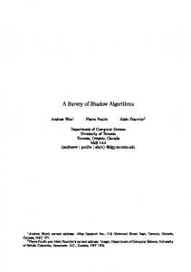
Fig. 3.1. Merging two sorted sequences. (a) The initial situation: The two lists are stored on disk. Two empty input buffers and an empty output buffer have been allocated in main memory. The output sequence does not contain any data yet. (b) The first block from each input sequence has been loaded into main memory. (c) The first B elements have been moved from the input buffers to the output buffer.
3. A Survey of Techniques for Designing I/O-Efficient Algorithms
(d) 2 4 7 8 12 16 19 27 37 44 48 61
7 8
39
1 3 5 11 17 21 22 35 40 55 57 62
5 11
1 2 3 4
(e) 2 4 7 8 12 16 19 27 37 44 48 61
12 16 19 27
1 3 5 11 17 21 22 35 40 55 57 62
11 5 7 8
1 2 3 4
Fig. 3.1. (continued) (d) The contents of the output buffer are flushed to the output stream to make room for more data to be moved to the output buffer. (e) After moving elements 5, 7, and 8 to the output buffer, the input buffer for the first stream does not contain any more data items. Hence, the next block is read from the first input stream into the input buffer.
array A� from array A takes O(N/B) I/Os rather than Θ(N ) I/Os, as would be required to solve this task using direct disk accesses. In our example we apply the scanning paradigm to a problem with one input stream A and one output stream A� . It is easy to apply the above buffering technique to a problem with q input streams S1 , . . . , Sq and r output streams S1� , . . . , Sr� , as long as there is enough room to keep an input buffer of size B per input stream Si and an output buffer of size B per output stream Sj� in internal memory. More precisely, p + q cannot be more than M/B. � Under this � assumption the algorithm still takes O(N/B) I/Os, where N = qi=1 |Si | + rj=1 |Sj� |. Note, however, that this analysis includes only the number of I/Os required to read the elements from the input streams and write the output to the output streams. It does not include the I/Ocomplexity of the actual computation of the output elements from the input elements. One way to guarantee that the I/O-complexity of the whole algorithm, including all computation, is O(N/B) is to ensure that only the M −(q +r)B elements most recently read from the input streams are required
40
Anil Maheshwari and Norbert Zeh
for the computation of the next output element, or the required information about all elements read from the input streams can be maintained succinctly in M − (q + r)B space. If this can be guaranteed, the computation of all output elements from the read input elements can be carried out in main memory and thus does not cause any I/O-operations to be performed. An important example where the scanning paradigm is applied to more than one input stream is the merging of k sorted streams to produce a single sorted output stream (see Fig. 3.1). This procedure is applied repeatedly with a parameter of k = 2 in the classical internal memory MergeSort algorithm. The I/O-efficient MergeSort algorithm discussed in the next section takes advantage of the fact that up to k = M/B streams can be merged in a linear number of I/Os, in order to decrease the number of recursive merge steps required to produce a single sorted output stream. 3.2.2 Sorting Sorting is a fundamental problem that arises in almost all areas of computer science, including large scale applications such as database systems. Besides the obvious applications where the task at hand requires per definition that the output be produced in sorted order, sorting is often applied as a paradigm for eliminating random disk accesses in external memory algorithms. Consider for instance a graph algorithm that performs a traversal of the input graph to compute a labelling of its vertices. This task does not require any part of the representation of the graph to be sorted, so that the internal memory algorithm does not necessarily include a sorting step. An external memory algorithm for the same problem, on the other hand, can benefit greatly by sorting the vertex set of the graph appropriately. In particular, without sorting the vertex set, the algorithm has no control over the order in which the vertices are stored on disk. Hence, in the worst case the algorithm spends one I/O to load each vertex into internal memory when it is visited. If the order in which the vertices of the graph are visited can be determined efficiently, it is more efficient to sort the vertices in this order and then perform the traversal of the graph using a simple scan of the sorted vertex set. The number of I/O-efficient sorting algorithms that have been proposed in the literature is too big for us to give an exhaustive survey of these algorithms at the level of detail appropriate for a tutorial as this one. Hence, we restrict our discussion to a short description of the two main paradigms applied in I/O-efficient sorting algorithms and then present the simplest I/O-optimal sorting algorithm in detail. At the end of this section we discuss a number of issues that need to be addressed in order to obtain I/O-optimal algorithms for sorting on multiple disks. Besides algorithms that delegate the actual work required to sort the given set of data elements to I/O-efficient data structures, the existing sorting algorithms can be divided into two categories based on the basic approach taken to produce the sorted output.
3. A Survey of Techniques for Designing I/O-Efficient Algorithms
41
Algorithms based on the merging paradigm proceed in two phases. In the first phase, the run formation phase, the input data is partitioned into more or less trivial sorted sequences, called “runs”. In the second phase, the merging phase, these runs are merged until only one sorted run remains, where merging k runs S1 , . . . , Sk means that a single sorted run S � is produced that contains all elements of runs S1 , . . . , Sk . The classical internal memory MergeSort algorithm is probably the simplest representative of this class of algorithms. The run formation phase is trivial in this case, as it simply declares every input element to be in a run of its own. The merging phase uses two-way merging to produce longer runs from shorter ones. That is, given the current set of runs S1 , . . . , Sk , these runs are grouped into pairs of runs and each pair is merged to form a longer run. Each such iteration of merging pairs of runs can be carried out in linear time. The number of runs reduces by a factor of two from one iteration to the next, so that O(log N ) iterations suffice to produce a single sorted run containing all data elements. Hence, the algorithm takes O(N log N ) time. Algorithms based on the distribution paradigm compute a partition of the given data set S into subsets S0 , . . . , Sk so that for all 0 ≤ i < j ≤ k and any two elements x ∈ Si and y ∈ Sj , x ≤ y. Given this partition, a sequence containing the elements of S in sorted order is produced by sorting each of the sets S0 , . . . , Sk recursively and concatenating the resulting sorted sequences. In order to produce sets S0 , . . . , Sk , the algorithm chooses a set of splitters x1 ≤ · · · ≤ xk from S. To simplify the discussion, we also assume that there are two splitters x0 = −∞ and xk+1 = +∞. Then set Si , 0 ≤ i ≤ k, is defined as the set of elements y ∈ S so that xi ≤ y < xi+1 . Given the set of splitters, sets S0 , . . . , Sk are produced by comparing each element in S to the splitters. The efficiency of this procedure depends on a good choice of the splitter elements. If it can be guaranteed that each of the sets S0 , . . . , Sk has size O(|S|/k), the procedure finishes in O(N log2 N ) time because O(logk N ) levels of recursion suffice to produce a partition of the input into N singleton sets that are arranged in the right order, and each level of recursion takes O(N log k) time to compare each element in S to the splitters. QuickSort is a representative of this class of algorithms. In internal memory MergeSort has the appealing property of being simpler than QuickSort because the run formation phase is trivial and the merging phase is a simple iterative process that requires only little bookkeeping. In contrast, QuickSort faces the problem of computing a good splitter, which is easy using randomization, but requires some effort if done deterministically. In external memory the situation is not much different, as long as the goal is to sort optimally on a single disk. If I/O-optimal performance is to be achieved on multiple disks, distribution-based algorithms are preferable because it is somewhat easier to make them take full advantage of the parallel nature of multi-disk systems. Since we do not go into too much detail discussing the issues involved in optimal sorting on multiple disks, we
42
Anil Maheshwari and Norbert Zeh
choose an I/O-efficient version of MergeSort as the sorting algorithm we discuss in detail. The algorithm is simple, resembles very much the internal memory algorithm, and achieves optimal performance on a single disk. In order to see what needs to be done to obtain a MergeSort algorithm that performs O((N/B) logM/B (N/B)) I/Os, let us analyze the I/Ocomplexity of the internal memory MergeSort algorithm as it is. The run formation phase does not require any I/Os. Merging two sorted runs S1 and S2 takes O(1 + (|S1 | + |S2 |)/B) I/Os using the scanning paradigm: Read the first element from each of the two streams. Let x and y be the two read elements. If x < y, place x into the output stream, read the next element from S1 , and repeat the whole procedure. If x ≥ y, place y into the output stream, read the next element from S2 , and repeat the whole procedure. Since every input element is involved in O(log N ) merge steps, and the total number of merge steps is O(N ), the I/O-complexity of the internal memory MergeSort algorithm is O(N + (N/B) log2 N ). The I/O-complexity of the algorithm can be reduced to O((N/B)· log2 (N/B)) by investing O(N/B) I/Os during the run formation phase. In particular, the run formation phase makes sure that the merge phase starts out with N/M sorted runs of length M instead of N singleton runs. To achieve this goal, the data is partitioned into N/M chunks of size M . Then each chunk is loaded into main memory, sorted internally, and written back to disk in sorted order. Reading and writing each chunk takes O(M/B) I/Os, so that the total I/O-complexity of the run formation phase is O(N/M ·M/B) = O(N/B). As a result of reducing the number of runs to N/M , the merge phase now takes O(N/M + (N/B) log2 (N/M )) = O((N/B) log2 (N/B)) I/Os. In order to increase the base of the logarithm to M/B, it has to be ensured that the number of runs reduces by a factor of Ω(M/B) from one iteration of the merge phase to the next because then O(logM/B (N/B)) iterations suffice to produce a single sorted run. In order to achieve this goal, the obvious thing to do is to merge k = M/(2B) runs S1 , . . . , Sk instead of only two runs in a single merge step. Similar to the internal memory merge step, the algorithm loads the first elements x1 , . . . , xk from runs S1 , . . . , Sk into main memory, copies the smallest of them, xi , to the output run, reads the next element from Si and repeats the whole procedure. The I/O-complexity of this �k modified merge step is O(k + ( i=1 |Si |)/B) because the available amount of main memory suffices to allocate a buffer of size B for each input and output run, so that the scanning paradigm can be applied. Using this modified merge step, the number of runs reduces by a factor of M/(2B) from one iteration of the merge phase to the next. Hence, the algorithm produces a single sorted run already after O(logM/B (N/B)) iterations, and the I/O-complexity of the algorithm becomes O((N/B) logM/B (N/B)), as desired. An issue that does not affect the I/O-complexity of the algorithm, but is important to obtain a fast algorithm, is how the merging of k runs instead
3. A Survey of Techniques for Designing I/O-Efficient Algorithms
43
of two runs is done in internal memory. When merging two runs, choosing the next element to be moved to the output run involves a single comparison. When merging k > 2 runs, it becomes computationally too expensive to find the minimum of elements x1 , . . . , xk in O(k) time because then the running time of the merge phase would be O(kN logk (N/B)). In order to achieve optimal running time in internal memory as well, the minimum of elements x1 , . . . , xk has to be found in O(log k) time. This can be achieved by maintaining the smallest elements x1 , . . . , xk , one from each run, in a priority queue. The next element to be moved to the output run is the smallest in the priority queue and can hence be retrieved using a DeleteMin operation. Let the retrieved element be xi ∈ Si . Then after moving xi to the output run, the next element is read from Si and inserted into the priority queue, which guarantees that again the smallest unprocessed element from every run is stored in the priority queue. This process is repeated until all elements have been moved to the output run. The amount of space used by the priority queue is O(k) = O(M/B), so that the priorty queue can be maintained in main memory. Moving one element to the output run involves the execution of one DeleteMin and one Insert operation on the priority queue, which takes O(log k) time. Hence, the total running time of the MergeSort algorithm is O(N log M + (N log k) logk (N/B)) = O(N log N ). We summarize the discussion in the following theorem. Theorem 3.1. [17] A set of N elements can be sorted using O((N/B) logM/B (N/B)) I/Os and O(N log N ) internal memory computation time. Sorting optimally on multiple disks is a more challenging problem. The challenge with distribution-based algorithms is to distribute the blocks of the buckets approximately evenly across the D disks while at the same time making sure that every I/O-operation writes Ω(D) blocks to disk. The latter requirement needs to be satisfied to guarantee that the algorithm takes full advantage of the parallel disks (up to a constant factor) during write operations. The former requirement is necessary to guarantee that the recursive invocation of the sorting algorithm can utilize the full bandwidth of the parallel I/O-system when reading the data elements to be sorted. Vitter and Shriver [755] propose randomized online techniques that guarantee that with high probability each bucket is distributed evenly across the D disks. The balancing algorithm applies the classical result that if α balls are placed uniformly at random into β bins and α = Ω(β log β), then all bins contain approximately the same number of balls, with high probability. The balancing algorithm maps the blocks of each bucket uniformly at random to disks where they are to be stored. Viewing the blocks in a bucket as balls and the disks as bins, and assuming that the number of blocks is sufficiently larger than the number of disks, the blocks in each bucket are distributed evenly across the D disks, with high probability. A number of deterministic methods for
44
Anil Maheshwari and Norbert Zeh
performing distribution sort on multiple disks have also been proposed, including BalanceSort [586], sorting using the buffer tree [52], and algorithms obtained by simulating bulk-synchronous parallel sorting algorithms [244]. The reader may refer to these references for details. For merge sort, it is required that each iteration in the merging phase is carried out in O(N/(DB)) I/Os. In particular, each read operation must bring Ω(D) blocks of data into main memory, and each write operation must write Ω(D) blocks to disk. While the latter is easy to achieve, reading blocks in parallel is difficult because the runs to be merged were formed in the previous iteration without any knowledge about how they would interact with other runs in subsequent merge operations. Nodine and Vitter [587] propose an optimal deterministic merge sort for multiple disks. The algorithm first performs an approximate merge phase that guarantees that no element is too far away from its final location. In the second phase, each element is moved to its final location. Barve et al. [92, 93] claim that their sorting algorithm is the most practical one. Using their approach, each run is striped across the disks, with a random starting disk. When merging runs, the next block needed from each disk is read into main memory. If there is not sufficient room in main memory for all the blocks to be read, then the least needed blocks are discarded from main memory (without incurring any I/Os). They derive asymptotic upper bounds on the expected I/O complexity of their algorithm.
3.3 Simulation of Parallel Algorithms in External Memory Blockwise data access is a central theme in the design of I/O-efficient algorithms. A second important issue, when more than one disk is present, is fully parallel disk I/O. A number of techniques have been proposed that address this issue by simulating parallel algorithms as external memory algorithms. Most notably, Atallah and Tsay [74] discuss how to derive I/O-efficient algorithms from parallel algorithms for mesh architectures, Chiang et al. [192] discuss how to obtain I/O-efficient algorithms from PRAM algorithms, and Sibeyn and Kaufmann [692], Dehne et al. [242, 244], and Dittrich et al. [254] discuss how to simulate coarse-grained parallel algorithms developed for the BSP, CGM, and BSP∗ models in external memory. In this section we discuss the simulation of PRAM algorithms in external memory, which has been proposed by Chiang et al. [192]. For a discussion of other simulation results see Chapter 15. The PRAM simulation of [192] is particularly appealing as it translates the large number of PRAM-algorithms described in the literature into I/Oefficient and sometimes I/O-optimal algorithms, including algorithms for a large number of graph and geometric problems, such as connectivity, computing minimum spanning trees, planarity testing and planar embedding,
3. A Survey of Techniques for Designing I/O-Efficient Algorithms
45
computing convex hulls, Voronoi diagrams, and triangulations of point sets in the plane. In order to describe the simulation paradigm of [192], let us quickly recall the definition of a PRAM. A PRAM consists of a number of RAM-type processing units that operate synchronously and share a global memory. Different processors can exchange information by reading and writing the same memory cell in the shared memory. The two main measures of performance of an algorithm in the PRAM-model are its running time and the amount of work it performs. The former is defined as the maximum number of computation steps performed by any of the processors. The latter is the product of the running time of the algorithm times the number of processors. Now consider a PRAM-algorithm A that uses N processors and O(N ) space and runs in O(T (N )) time. To simulate the computation of algorithm A, assume that the processor contexts (O(1) state information per processor) and the content of the shared memory are stored on disk in a suitable format. Assume furthermore that every computation step of a processor consists of a constant number of read accesses to shared memory (to retrieve the operands of the computation step), followed by O(1) computation, and a constant number of write accesses to shared memory (to write the results back to memory). Then one step of algorithm A can be simulated in O(sort(N )) I/Os as follows: First scan the list of processor contexts to translate the read accesses each processor intends to perform into read requests that are written to disk. Then sort the resulting list of read requests by the memory locations they access. Scan the sorted list of read requests and the memory representation to augment every read request with the content of the memory cell it addresses. Sort the list of read requests again, this time by the issuing processor, and finally scan the sorted list of read requests and the list of processor contexts to transfer the requested operands to each processor. The computation of all processors can now be simulated in a single scan over the processor contexts. Writing the results of the computation to the shared memory can be simulated in a manner similar to the simulation of reading the operands. The simulation of read and write accesses to the shared memory requires O(1) scans of the list of processor contexts, O(1) scans of the representation of the shared memory, and sorting and scanning the lists of read and write requests a constant number of times. Since all these lists have size O(N ), this takes O(sort(N )) I/Os. As argued above, the computation itself can be carried out in O(scan(N )) I/Os. Hence, a single step of algorithm A can be simulated in O(sort(N )) I/Os, so that simulating the whole algorithm takes O(T (N ) · sort(N )) I/Os. Theorem 3.2. [192] A PRAM algorithm that uses N processors and O(N ) space and runs in time T (N ) can be simulated in O(T (N ) · sort(N )) I/Os.
46
Anil Maheshwari and Norbert Zeh ∗
48 −
+ ∗
/
4
2
2
7
8
2
1
3
(a)
6
4
7
6
2
2
1
3
(b)
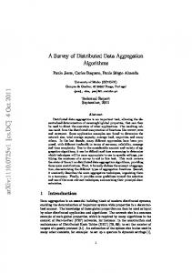
Fig. 3.2. (a) The expression tree for the expression ((4 / 2) + (2 ∗ 3)) ∗ (7 − 1). (b) The same tree with its vertices labelled with their values..
An interesting situation arises when the number of active processors and the amount of data to be processed decrease geometrically. That is, after a constant number of steps, the number of active processors and the amount of processed data decrease by a constant factor. Then the data and the contexts of the active processors can be compacted after each PRAM step, so that the I/O-complexity of simulating the steps of the algorithm is also geometrically decreasing. This implies that the I/O-complexity of the algorithm is dominated by the complexity of simulating the first step of the algorithm, which is O(sort(N )).
3.4 Time-Forward Processing Time-forward processing [52, 192] is an elegant technique for solving problems that can be expressed as a traversal of a directed acyclic graph (DAG) from its sources to its sinks. Problems of this type arise mostly in I/O-efficient graph algorithms, even though applications of this technique for the construction of I/O-efficient data structures are also known. Formally, the problem that can be solved using time-forward processing is that of evaluating a DAG G: Let φ be an assignment of labels φ(v) to the vertices of G. Then the goal is to compute another labelling ψ of the vertices of G so that for every vertex v ∈ G, label ψ(v) can be computed from labels φ(v) and ψ(u1 ), . . . , ψ(uk ), where u1 , . . . , uk are the in-neighbors of v. As an illustration, consider the problem of expression-tree evaluation (see Fig. 3.2). For this problem, the input is a binary tree T whose leaves store real numbers and whose internal vertices are labelled with one of the four elementary binary operations +, −, ∗, /. The value of a vertex is defined recursively. For a leaf v, its value val (v) is the real number stored at v. For an
3. A Survey of Techniques for Designing I/O-Efficient Algorithms
47
internal vertex v with label ◦ ∈ {+, −, ∗, /}, left child x, and right child y, val (v) = val (x) ◦ val (y). The goal is to compute the value of the root of T . Cast in terms of the general DAG evaluation problem defined above, tree T is a DAG whose edges are directed from children to parents, labelling φ is the initial assignment of real numbers to the leaves of T and of operations to the internal vertices of T , and labelling ψ is the assignment of the values val (v) to all vertices v ∈ T . For every vertex v ∈ T , its label ψ(v) = val (v) is computed from the labels ψ(x) = val (x) and ψ(y) = val (y) of its in-neighbors (children) and its own label φ(v) ∈ {+, −, ∗, /}. In order to be able to evaluate a DAG G I/O-efficiently, two assumptions have to be satisfied: (1) The vertices of G have to be stored in topologically sorted order. That is, for every edge (v, w) ∈ G, vertex v precedes vertex w. (2) Label ψ(v) has to be computable from labels φ(v) and ψ(u1 ), . . . , ψ(uk ) in O(sort(k)) I/Os. The second condition is trivially satisfied if every vertex of G has in-degree no more than M . Given these two assumptions, time-forward processing visits the vertices of G in topologically sorted order to compute labelling ψ. Visiting the vertices of G in this order guarantees that for every vertex v ∈ G, its in-neighbors are evaluated before v is evaluated. Thus, if these in-neighbors “send” their labels ψ(u1 ), . . . , ψ(uk ) to v, v has these labels and its own label φ(v) at its disposal to compute ψ(v). After computing ψ(v), v sends its own label ψ(v) “forward in time” to its out-neighbors, which guarantees that these out-neighbors have ψ(v) at their disposal when it is their turn to be evaluated. The implementation of this technique due to Arge [52] is simple and elegant. The “sending” of information is realized using a priority queue Q (see Chapter 2 for a discussion of priority queues). When a vertex v wants to send its label ψ(v) to another vertex w, it inserts ψ(v) into priority queue Q and gives it priority w. When vertex w is evaluated, it removes all entries with priority w from Q. Since every in-neighbor of w sends its label to w by queuing it with priority w, this provides w with the required inputs. Moreover, every vertex removes its inputs from the priority queue before it is evaluated, and all vertices with smaller numbers are evaluated before w. Thus, at the time when w is evaluated, the entries in Q with priority w are those with lowest priority, so that they can be removed using a sequence of DeleteMin operations. Using the buffer tree of Arge [52] to implement priority queue Q, Insert and DeleteMin operations on Q can be performed in O((1/B)· logM/B (|E|/B)) I/Os amortized because priority queue Q never holds more than |E| entries. The total number of priority queue operations performed by the algorithm is O(|E|), one Insert and one DeleteMin operation per edge. Hence, all updates of priority queue Q can be processed in O(sort(|E|)) I/Os. The computation of labels ψ(v) from labels φ(v) and ψ(u1 ), . . . , ψ(uk ), for all vertices v ∈ G, can also be carried out in O(sort(|E|)) I/Os, using the
48
Anil Maheshwari and Norbert Zeh
above assumption that this computation takes O(sort(k)) I/Os for a single vertex v. Hence, we obtain the following result. Theorem 3.3. [52, 192] Given a DAG G = (V, E) whose vertices are stored in topologically sorted order, graph G can be evaluated in O(sort(|V | + |E|)) I/Os, provided that the computation of the label of every vertex v ∈ G can be carried out in O(sort(deg− (v))) I/Os, where deg− (v) is the in-degree of vertex v.
3.5 Greedy Graph Algorithms In this section we describe a simple technique proposed in [775] that can be used to make internal memory graph algorithms of a sufficiently simple structure I/O-efficient. For this technique to be applicable, the algorithm has to compute a labelling of the vertices of the graph, and it has to do so in a particular way. We call a vertex labelling algorithm A single-pass if it computes the desired labelling λ of the vertices of the graph by visiting every vertex exactly once and assigns label λ(v) to v during this visit. We call A local if label λ(v) can be computed in O(sort(k)) I/Os from labels λ(u1 ), . . . , λ(uk ), where u1 , . . . , uk are the neighbors of v whose labels are computed before λ(v). Finally, algorithm A is presortable if there is an algorithm that takes O(sort(|V | + |E|)) I/Os to compute an order of the vertices of the graph so that A produces a correct result if it visits the vertices of the graph in this order. The technique we describe here is applicable if algorithm A is presortable, local, and single-pass. So let A be a presortable local single-pass vertex-labelling algorithm computing some labelling λ of the vertices of a graph G = (V, E). In order to make algorithm A I/O-efficient, the two main problems are to determine an order in which algorithm A should visit the vertices of G and devise a mechanism that provides every vertex v with the labels of its previously visited neighbors u1 , . . . , uk . Since algorithm A is presortable, there exists an algorithm A� that takes O(sort(|V | + |E|)) I/Os to compute an order of the vertices of G so that algorithm A produces the correct result if it visits the vertices of G in this order. Assume w.l.o.g. that this ordering of the vertices of G is expressed as a numbering. We use algorithm A� to number the vertices of G and then derive a DAG G� from G by directing every edge of G from the vertex with smaller number to the vertex with larger number. DAG G� has the property that for every vertex v, the in-neighbors of v in G� are exactly those neighbors of v that are labelled before v. Hence, labelling λ can be computed using time-forward processing. In particular, by the locality of A, the label λ(v) of every vertex can be computed in O(sort(k)) I/Os from the labels λ(u1 ), . . . , λ(uk ) of its in-neighbors u1 , . . . , uk in G� , which is a simplified version of the condition for the applicability of time-forward processing. This leads to the following result.
3. A Survey of Techniques for Designing I/O-Efficient Algorithms
49
Theorem 3.4. [775] Every graph problem P that can be solved by a presortable local single-pass vertex labelling algorithm can be solved in O(sort(|V |+ |E|)) I/Os. An important observation to be made is that in this application of timeforward processing, the restriction that the vertices of the DAG to be evaluated have to be given in topologically sorted order does not pose a problem because the directions of the edges are chosen only after fixing an order of the vertices that is to be the topological order. To illustrate the power of Theorem 3.4, we apply it below to obtain deterministic O(sort(|V |+|E|)) I/O algorithms for finding a maximal independent set of a graph G and coloring a graph of degree ∆ with ∆ + 1 colors. In [775], the approach is applied in a less obvious manner in order to compute a maximal matching of a graph G = (V, E) in O(sort(|V | + |E|)) I/Os. The problem with computing a maximal matching is that it is an edge labelling problem. However, Zeh [775] shows that it can be transformed into a vertex labelling problem of a graph with |E| vertices and at most 2|E| edges. 3.5.1 Computing a Maximal Independent Set In order to compute a maximal independent set S of a graph G = (V, E) in internal memory, the following simple algorithm can be used: Process the vertices in an arbitrary order. When a vertex v ∈ V is visited, add it to S if none of its neighbors is in S. Translated into a labelling problem, the goal is to compute the characteristic function χS : V → {0, 1} of S, where χS (v) = 1 if v ∈ S, and χS (v) = 0 if v ∈ S. Also note that if S is initially empty, then any neighbor w of v that is visited after v cannot be in S at the time when v is visited, so that it is sufficient for v to inspect all its neighbors that are visited before v to decide whether or not v should be added to S. The result of these modifications is a vertex-labelling algorithm that is presortable (since the order in which the vertices are visited is unimportant), local (since only previously visited neighbors of v are inspected to decide whether v should be added to S, and a single scan of labels χS (u1 ), . . . , χS (uk ) suffices to do so), and single-pass. This leads to the following result. Theorem 3.5. [775] Given an undirected graph G = (V, E), a maximal independent set of G can be found in O(sort(|V | + |E|)) I/Os and linear space. 3.5.2 Coloring Graphs of Bounded Degree The algorithm to compute a (∆ + 1)-coloring of a graph G whose vertices have degree bounded by some constant ∆ is similar to the algorithm for computing a maximal independent set presented in the previous section: Process the vertices in an arbitrary order. When a vertex v ∈ V is visited, assign a
50
Anil Maheshwari and Norbert Zeh
color c(v) ∈ {1, . . . , ∆+1} to vertex v that has not been assigned to any neighbor of v. The algorithm is presortable and single-pass for the same reasons as the maximal independent set algorithm. The algorithm is local because the color of v can be determined as follows: Sort the colors c(u1 ), . . . , c(uk ) of v’s in-neighbors u1 , . . . , uk . Then scan this list and assign the first color not in this list to v. This takes O(sort(k)) I/Os. Theorem 3.6. [775] Given an undirected graph G = (V, E) whose vertices have degree at most ∆, a (∆ + 1)-coloring of G can be computed in O(sort(|V | + |E|)) I/Os and linear space.
3.6 List Ranking and the Euler Tour Technique List ranking and the Euler tour technique are two techniques that have been applied successfully in the design of PRAM algorithms for labelling problems on lists and rooted trees and problems that can be reduced efficiently to one of these problems. Given the similarity of the issues to be addressed in parallel and external memory algorithms, it is not surprising that the same two techniques can be applied in I/O-efficient algorithms as well. 3.6.1 List Ranking Let L be a linked list, i.e., a collection of vertices x1 , . . . , xN such that each vertex xi , except the tail of the list, stores a pointer succ(xi ) to its successor in L, no two vertices have the same successor, and every vertex can reach the tail of L by following successor pointers. Given a pointer to the head of the list (i.e., the vertex that no other vertex in the list points to), the list ranking problem is that of computing for every vertex xi of list L, its distance from the head of L, i.e., the number of edges on the path from the head of L to xi . In internal memory this problem can easily be solved in linear time using the following algorithm: Starting at the head of the list, follow successor pointers and number the vertices of the list from 0 to N − 1 in the order they are visited. Often we use the term “list ranking” to denote the following generalization of the list ranking problem, which is solvable in linear time using a straightforward generalization of the above algorithm: Given a function λ : {x1 , . . . , xN } → X assigning labels to the vertices of list L and a multiplication ⊗ : X × X → X defined �over X, � compute � � = λ xσ(1) and vertex x of L such that φ x a �label�φ(xi )� for each σ(1) � � �i φ xσ(i) = φ xσ(i−1) ⊗ λ xσ(i) , for 1 < i ≤ N , where�σ : [1,� N ] → [1, N ] is a permutation so that xσ(1) is the head of L and succ xσ(i) = xσ(i+1) , for 1 ≤ i < N. Unfortunately the simple internal memory algorithm is not I/O-efficient: Since we have no control over the physical order of the vertices of L on disk,
3. A Survey of Techniques for Designing I/O-Efficient Algorithms
51
an adversary can easily arrange the vertices of L in a manner that forces the internal memory algorithm to perform one I/O per visited vertex, so that the algorithm performs Ω(N ) I/Os in total. On the other hand, the lower bound for list ranking shown in [192] is only Ω(perm(N )). Next we sketch a list ranking algorithm proposed in [192] that takes O(sort(N )) I/Os and thereby closes the gap between the lower and the upper bound. We make the simplifying assumption that multiplication over X is associative. If this is not the case, we determine the distance of every vertex from the head of L, sort the vertices of L by increasing distances, and then compute the prefix product using the internal memory algorithm. After arranging the vertices by increasing distances from the head of L, the internal memory algorithm takes O(scan(N )) I/Os. Hence, the whole procedure still takes O(sort(N )) I/Os, and the associativity assumption is not a restriction. Given that multiplication over X is associative, the algorithm of [192] uses graph contraction to rank list L as follows: First an independent set I of L is found so that |I| = Ω(N ). Then the elements in I are removed from L. That is, for every element x ∈ I with predecessor y and successor z in L, the successor pointer of y is updated to succ(y) = z. The label of x is multiplied with the label of z, and the result is assigned to z as its new label in the compressed list. It is not hard to see that the weighted ranks of the elements in L−I remain the same after adjusting the labels in this manner. Hence, their ranks can be computed by applying the list ranking algorithm recursively to the compressed list. Once the ranks of all elements in L − I are known, the ranks of the elements in I are computed by multiplying their labels with the ranks of their predecessors in L. If the algorithm excluding the recursive invocation on the compressed list takes O(sort(N )) I/Os, the total I/O-complexity of the algorithm is given by the recurrence I(N ) = I(cN )+O(sort(N )), for some constant 0 < c < 1. The solution of this recurrence is O(sort(N )). Hence, we have to argue that every step, except the recursive invocation, can be carried out in O(sort(N )) I/Os. Given independent set I, it suffices to sort the vertices in I by their successors and the vertices in L − I by their own IDs, and then scan the resulting two sorted lists to update the weights of the successors of all elements in I. The successor pointers of the predecessors of all elements in I can be updated in the same manner. In particular, it suffices to sort the vertices in L − I by their successors and the vertices in I by their own IDs, and then scan the two sorted lists to copy the successor pointer from each vertex in I to its predecessor. Thus, the construction of the compressed list takes O(sort(N )) I/Os, once set I is given. In order to compute the independent set I, Chiang et al. [192] apply a 3-coloring procedure for lists, which applies time-forward processing to “monotone” sublists of L and takes O(sort(N )) I/Os; the largest monochromatic set is chosen to be set I. Using the maximal independent set algorithm of Section 3.5.1, a large independent set I can be obtained more directly in
52
Anil Maheshwari and Norbert Zeh
the same number of I/Os because a maximal independent set of a list has size at least N/3. Thus, we have the following result. Theorem 3.7. [192] A list of length N can be ranked in O(sort(N )) I/Os. List ranking alone is of very limited use. However, combined with the Euler tour technique described in the next section, it becomes a very powerful tool for solving problems on trees that can be expressed as functions over a traversal of the tree or problems on general graphs that can be expressed in terms of a traversal of a spanning tree of the graph. An important application is the rooting of an undirected tree T , which is the process of directing all edges of T from parents to children after choosing one vertex of T as the root. Given a rooted tree T (i.e., one where all edges are directed from parents to children), the Euler tour technique and list ranking can be used to compute a preorder or postorder numbering of the vertices of T , or the sizes of the subtrees rooted at the vertices of T . Such labellings are used in many classical graph algorithms, so that the ability to compute them is a first step towards solving more complicated graph problems. 3.6.2 The Euler Tour Technique An Euler tour of a tree T = (V, E) is a traversal of T that traverses every edge exactly twice, once in each direction. Such a traversal is useful, as it produces a linear list of vertices or edges that captures the structure of the tree. Hence, it allows standard parallel or external memory algorithms to be applied to this list, in order to solve problems on tree T that can be expressed as some function to be evaluated over the Euler tour. Formally, the tour is represented as a linked list L whose elements are the edges in the set {(v, w), (w, v) : {v, w} ∈ E} and so that for any two consecutive edges e1 and e2 , the target of e1 is the source of e2 . In order to define an Euler tour, choose a circular order of the edges incident to each vertex of T . Let {v, w1 }, . . . , {v, wk } be the edges incident to vertex v. Then let succ((wi , v)) = (v, wi+1 ), for 1 ≤ i < k, and succ((wk , v)) = (v, w1 ). The result is a circular linked list of the edges in T . Now an Euler tour of T starting at some vertex r and returning to that vertex can be obtained by choosing an edge (v, r) with succ((v, r)) = (r, w), setting succ((v, r)) = null, and choosing (r, w) as the first edge of the traversal. List L can be computed from the edge set of T in O(sort(N )) I/Os: First scan set E to replace every edge {v, w} with two directed edges (v, w) and (w, v). Then sort the resulting set of directed edges by their target vertices. This stores the incoming edges of every vertex consecutively. Hence, a scan of the sorted edge list now suffices to compute the successor of every edge in L. Lemma 3.8. An Euler tour L of a tree with N vertices can be computed in O(sort(N )) I/Os.
3. A Survey of Techniques for Designing I/O-Efficient Algorithms
53
Given an unrooted (and undirected) tree T , choosing one vertex of T as the root defines a direction on the edges of T by requiring that every edge be directed from the parent to the child. The process of rooting tree T is that of computing these directions explicitly for all edges of T . To do this, we construct an Euler tour starting at an edge (r, v) and compute the rank of every edge in the list. For every pair of opposite edges (u, v) and (v, u), we call the edge with the lower rank a forward edge, and the other a back edge. Now it suffices to observe that for any vertex x = r in T , edge (parent (x), x) is traversed before edge (x, parent (x)) by any Euler tour starting at r. Hence, for every pair of adjacent vertices x and parent (x), edge (parent (x), x) is a forward edge, and edge (x, parent (x)) is a back edge. That is, the set of forward edges is the desired set of edges directed from parents to children. Constructing and ranking an Euler tour starting at the root r takes O(sort(N )) I/Os, by Theorem 3.7 and Lemma 3.8. Given the ranks of all edges, the set of forward edges can be extracted by sorting all edges in L so that for any two adjacent vertices v and w, edges (v, w) and (w, v) are stored consecutively and then scanning this sorted edge list to discard the edge with higher rank from each of these edge pairs. Hence, a tree T can be rooted in O(sort(N )) I/Os. Instead of discarding back edges, it may be useful to keep them, but tag every edge of the Euler tour L as either a forward or back edge. Using this information, well-known labellings of the vertices of T can be computed by ranking list L after assigning appropriate weights to the edges of L. For example, consider the weighted ranks of the edges in L after assigning weight one to every forward edge and weight zero to every back edge. Then the preorder number of every vertex v = r in T is one more than the weighted rank of the forward edge with target v; the preorder number of the root r is always one. The size of the subtree rooted at v is one more than the difference between the weighted ranks of the back edge with source v and the forward edge with target v. To compute a postorder numbering, we assign weight zero to every forward edge and weight one to every back edge. Then the postorder number of every vertex v = r is the weighted rank of the back edge with source v. The postorder number of the root r is always N . After labelling every edge in L as a forward or back edge, the appropriate weights for computing the above labellings can be assigned in a single scan of list L. The weighted ranks can then be computed in O(sort(N )) I/Os, by Theorem 3.7. Extracting preorder and postorder numbers from these ranks takes a single scan of list L again. To extract the sizes of the subtrees rooted at the vertices of T , we sort the edges in L so that opposite edges with the same endpoints are stored consecutively. Then a single scan of this sorted edge list suffices to compute the size of the subtree rooted at every vertex v. Hence, all these labels can be computed in O(sort(N )) I/Os for a tree with N vertices.
54
Anil Maheshwari and Norbert Zeh
3.7 Graph Blocking The final topic we consider is that of blocking graphs. In particular, we are interested in laying out graphs on disk so that traversals of paths in these graphs cause as few page faults as possible, using an appropriate paging algorithm that needs to be specified along with the graph layout. We make two assumptions the first of which makes the design of suitable layouts easier, while the second makes it harder. The first assumption we make is that the graph to be stored on disk is static, i.e., does not change. Hence, it is not necessary to be able to update the graph I/O-efficiently, so that redundancy can be used to obtain better layouts. That is, some or all of the vertices of the graph may be stored in more than one location on disk. In order to visit such a vertex v, it suffices to visit any of these copies. This gives the paging algorithm considerable freedom in choosing the “best” of all disk blocks containing a copy of v as the one to be brought into main memory. By choosing the right block, the paging algorithm can guarantee that the next so many steps along the path do not cause any page faults. The second assumption we make is that the paths are traversed in an online fashion. That is, the traversed path is constructed only while it is traversed and is not known in advance. This allows an adversary to choose the worst possible path based on the previous decisions made by the paging algorithm, and the paging algorithm has to be able to handle such adversarial behavior gracefully. That is, it has to minimize the number of page faults in the worst case without having any a priori knowledge about the traversed path. Besides the obvious applications where the problem to be solved is a graph problem and the answer to a query consists of a traversal of a path in the graph, the theory of graph blocking can be applied in order to store pointerbased data structures on disk so that queries on these data structures can be answered I/O-efficiently. In particular, a pointer-based data structure can be viewed as a graph with additional information attached to its vertices. Answering a query on such a data structure often reduces to traversing a path starting at a specified vertex in the data structure. For example, laying out binary search trees on disk so that paths can be traversed I/O-efficiently, one arrives at a layout which bears considerable resemblance to a B-tree. As discussed in Chapter 2, the layout of lists discussed below needs only few modifications to be transformed into an I/O-efficient linked list data structure that allows insertions and deletions, i.e., is no longer static. Since we allow redundant representations of the graph, the two main measures of performance for a given blocking and the used paging algorithm are the number of page faults incurred by a path traversal in the worst case and the amount of space used by the graph representation. Clearly, in order to store a graph with N vertices on disk, at least N/B blocks of storage are required. We define the storage blow-up of a graph blocking to be β if it uses βN/B blocks of storage to store the graph on disk. Since space usage is a serious issue with large data sets, the goal is to design graph blockings that
3. A Survey of Techniques for Designing I/O-Efficient Algorithms
55
minimize the storage blow-up and at the same time minimize the number of page faults incurred by a path traversal. Often there is a trade-off. That is, no blocking manages to minimize both performance measures at the same time. In this section we restrict our attention to graph layouts with constant storage blow-up and bound the worst-case number of page faults achievable by these layouts using an appropriate paging algorithm. Throughout this section we denote the length of the traversed path by L. The traversal of such a path requires at least �L/B� I/Os in any graph because at most B vertices can be brought into main memory in a single I/O-operation. The graphs we consider include lists, trees, grids and planar graphs. The blocking for planar graphs generalizes to any class of graphs with small separators. The results presented here are described in detail in the papers of Nodine et al. [585], Hutchinson et al. [419], and Agarwal et al. [7]. Blocking Lists. The natural approach for blocking a list is to store the vertices of the list in an array, sorted in their order of appearance along the list. The storage blow-up of this blocking is one (i.e., there is no blow-up at all). Since every vertex is stored exactly once in the array, the paging algorithm has no choice about the block to be brought into main memory when a vertex is visited. Still, if the traversed path is simple (i.e., travels along the list in only one direction), the traversal of a path of length L incurs only L/B page faults. To see this, assume w.l.o.g. that the path traverses the list in forward direction, i.e., the vertices are visited in the same order as they are stored in the array, and consider a vertex v in the path that causes a page fault. Then v is the first vertex in the block that is brought into main memory, and the B − 1 vertices succeeding v in the direction of the traversal are stored in the same block. Hence, the traversal of any simple path causes one page fault every B steps along the path. If the traversed path is not simple, there are several alternatives. Assuming that M ≥ 2B, the same layout as for simple paths can be used; but the paging algorithm has to be changed somewhat. In particular, when a page fault occurs at a vertex v, the paging algorithm has to make sure that the block brought into main memory does not replace the block containing the vertex u visited just before v. Using this strategy, it is again guaranteed that after every page fault, at least B − 1 steps are required before the next page fault occurs. Indeed, the block containing vertex v contains all vertices that can be reached from v in B − 1 steps by continuing the traversal in the same direction, and the block containing vertex u contains all vertices that can be reached from v in B steps by continuing the traversal in the opposite direction. Hence, traversing a path of length L incurs at most L/B page faults. In the pathological situation that M = B (i.e., there is room for only one block in main memory) and given the layout described above, an adversary can construct a path whose traversal causes a page fault at every step. In particular, the adversary chooses two adjacent vertices v and w that are in
56
Anil Maheshwari and Norbert Zeh
v1 v2 v3 v4 v5 v6 v7 v8 v9 v10 v11 v12 v13 v14 v15 v16 v3 v4 v5 v6 v7 v8 v9 v10 v11 v12 v13 v14 Fig. 3.3. A layout of a list on a disk with block size B = 4. The storage blow-up of the layout is two.
different blocks and then constructs the path P = (v, w, v, w, . . . ). Whenever vertex v is visited, the block containing v is brought into main memory, thereby overwriting the block containing w. When vertex w is visited, the whole process is reversed. The following layout with storage blow-up two thwarts the adversary’s strategy: Instead of having only one array containing the vertices of the list, create a second array storing the vertices of the list in the same order, but with the block boundaries offset by B/2 (see Fig. 3.3). To use this layout efficiently, the paging algorithm has to change as follows: Assume that the current block is from the first array. When a page fault occurs, the vertex v to be visited is the last vertex in the block preceding the current block in the first array or the first vertex in the block succeeding the current block. Since the blocks in the second array are offset by B/2, this implies that v is at least B/2 − 1 steps away from the border of the block containing v in the second array. Hence, the paging algorithm loads this block into memory because then at least B/2 steps are required before the next page fault occurs. When the next page fault occurs, the algorithm switches back to a block in the first array, which again guarantees that the next B/2 − 1 steps cannot cause a page fault. That is, the paging algorithm alternates between the two arrays. Traversing a path of length L now incurs at most 2L/B page faults. Blocking Trees. Next we discuss blocking of trees. Quite surprisingly, trees cannot be blocked at all if there are no additional restrictions on the tree or the type of traversal that is allowed. To see this, consider a tree whose internal vertices have degree at least M . Then for any vertex v, at most M − 1 of its neighbors can reside in main memory at the same time as v. Hence, there is at least one neighbor of v that is not in main memory at the time when v is in main memory. An adversary would always select this vertex as the one to be visited after v. Since at least every other vertex on any path in the tree has to be an internal vertex, the adversary can construct a path that causes a page fault every other step along the path. Note that this is true irrespective of the storage blow-up of the graph representation. From this simple example it follows that for unrestricted traversals, a good blocking of a tree can be achieved only if the degree of the vertices of the tree is bounded by some constant d. We show that there is a blocking with storage blow-up four so that traversing a path of length L causes at most 2L/ logd B page faults. To construct this layout, which is very similar to the list layout
3. A Survey of Techniques for Designing I/O-Efficient Algorithms
57
logd B
logd B
Fig. 3.4. A blocking of a binary tree with block size 7. The subtrees in the first partition are outlined with dashed lines. The subtrees in the second partition are outlined with solid lines.
shown in Fig. 3.3, we choose one vertex r of T as the root and construct two partitions of T into layers of height logd B (see Fig. 3.4). In the first partition, the i-th layer contains all vertices at distance between (i − 1) logd B and i logd B − 1 from r. In the second partition, the i-th layer contains all vertices at distance between (i − 1/2) logd B and (i + 1/2) logd B = 1 from r. Each layer in both partitions consists of subtrees of size at most B, so that each subtree can be stored in a block. Moreover, small subtrees can be packed into blocks so that no block is less than half full. Hence, both partitions together use at most 4N/B blocks, and the storage blow-up is at most four. The paging algorithm now alternates between the two partitions similar to the above paging algorithm for lists. Consider the traversal of a path, and let v be a vertex that causes a page fault. Assume that the tree currently held in main memory is from the first partition. Then v is the root or a leaf of a tree in the first partition. Hence, the tree in the second partition that contains v contains all vertices that can be reached from v in (logd B)/2 − 1 steps. Thus, by loading this block into main memory, the algorithm guarantees that the next page fault occurs after at least (logd B)/2 − 1 steps, and traversing a path of length L causes at most 2L/(logd B) page faults. If all traversed paths are restricted to travel away from the root of T , the storage blow-up can be reduced to two, and the number of page faults can be reduced to L/ logd B. To see this, observe that only the first of the above partitions is needed, and for any traversed path, the vertices causing page faults are the roots of subtrees in the partition. After loading the block containing that root into main memory, logd B − 1 steps are necessary in order to reach a leaf of the subtree, and the next page fault occurs after logd B steps. For traversals towards the root, Hutchinson et al. [419] show that using O(N/B) disk blocks, a page fault occurs every Ω(B) steps, so that a path of length L can be traversed in O(L/B) I/Os.
58
Anil Maheshwari and Norbert Zeh
Blocking Two-Dimensional Grids. Blocking of two-dimensional grids can be done using the same ideas as for blocking lists. This is not too surprising because lists are equivalent to one-dimensional grids from a blocking point of view. In both cases, the grid is covered with subgrids of size B. In √ √ the two-dimensional case, the subgrids have dimension B × B. We call such a covering a tessellation. However, the added dimension does create a few complications. In particular, if the amount of main memory is M = B, a blocking that consists of three tessellations is required to guarantee that a page fault occurs only every ω(1) steps. To see that two tessellations are not sufficient, consider two tessellations offset by k and l in the �x√and y-dimensions. √ � � √Then an adversary √ � chooses a path containing vertices i B + k, j B , i B + k + 1, Bj , √ √ �√ � �√ � i B + k, j B + 1 , and i B + k + 1, j B + 1 , for two integers i and j. Neither of the two tessellations contains a subgrid that contains more than two of these vertices. Hence, given that the traversal is at one of the four vertices, and only one of the two subgrids containing this vertex is in main memory, an adversary can always choose the neighbor of the current vertex that does not belong to the subgrid in main memory. Thus, every step causes a page fault. By increasing the storage blow-up √ to three, it can be guaranteed that a page fault occurs at most every B/6 steps. In particular, the blocking √ consists of three tessellations so that the second tessellation has offset B/3 in both√directions w.r.t. the first tessellation, and the third tessellation has offset 2 B/3 w.r.t. the first tessellation (see Fig. 3.5). Then it is not hard to see that for every vertex in the grid, there exists at least √ one subgrid in one of the three tessellations, so that the vertex is at least B/6 steps away from the boundary of the subgrid. Hence, whenever a page fault occurs at some vertex v, the paging algorithm brings the appropriate grid for vertex v into main memory. If M ≥ 2B, the storage blow-up can be reduced √ to two, and the number of steps between two page faults can be increased to B/4. In particular, the blocking consists of two tessellations so that the second tessellation has offset √ B/2 in both directions w.r.t. the first tessellation. Let v be a vertex that causes a page fault, and let u be the vertex visited before v in the traversal. Then at the time when the paging algorithm has to bring vertex v into main memory, a block containing u from one of the two tessellations is already in main memory. Now it is easy to verify that the block containing u that is already in main memory together with one of √ the two blocks containing v in the two tessellations covers at least the B/4-neighborhood of v, i.e., the √ subgrid containing all vertices that can be reached from v in at most B/4 steps. Hence, by bringing the appropriate block containing v into main memory, the √ paging algorithm can guarantee that the next page fault occurs after only B/4 steps.
3. A Survey of Techniques for Designing I/O-Efficient Algorithms
59
Fig. 3.5. A blocking for M = B.
Finally, if M ≥ 3B, the storage blow-up can be brought down to one while keeping the number of page faults incurred by the traversal of a path √ of length L at 4L/ B. To achieve this, the tessellation shown in Fig. 3.6 √ is used. To prove that the traversal of a path of length L incurs at most 4L/ √ B page faults, we show that at most two page faults can occur within B/2 steps. So assume the opposite. Then let v be a vertex that causes a page fault, and let u be the vertex visited immediately before v. Let u be in the solid bold subgrid in Fig. 3.6 and assume that it is in the top √ left quarter of the subgrid. Then all vertices that can be reached from u in B/2 steps are contained in the solid thin subgrids. In particular, √ v is contained in one of these subgrids. If v is in subgrid A, it takes at least B/2 steps after visiting √ v to reach a vertex in subgrid C. If v is in subgrid C, it takes at least B/2 steps after visiting v to reach a vertex in subgrid A. Hence, in√both cases only a vertex in subgrid B can cause another page fault within B/2 steps after visiting vertex u. If v is in subgrid B,√consider the next vertex w after v that causes a page fault and is at most B/2 steps away from u. Vertex w is either in subgrid √ A, or in subgrid C. W.l.o.g. let w be in subgrid A. Then it takes at least B/2 steps to reach√a vertex in subgrid C, so that again only two page faults can occur within B/2 steps after visiting √ u. This shows that the traversal of a path of length L incurs at most 4L/ B page faults. Blocking Planar Graphs. The final result we discuss here concerns the blocking of planar graphs of bounded degree. Quite surprisingly, planar graphs allow blockings with the same performance as for trees, up to constant factors. That is, with constant storage blow-up it can be guaranteed that traversing a path of length L incurs at most 4L/ logd B page faults, where d is the maximal degree of the vertices in the graph. To achieve this, Agarwal et al. [7] make use of separator results due to Frederickson [315]. In particular,
60
Anil Maheshwari and Norbert Zeh
A B u
C
Fig. 3.6. A blocking with storage blow-up one.
Frederickson � √ � shows that for every planar graph G, there exists a set S of O N/ B vertices so that no connected component of G − S has size more than B. Based on this result, the following graph representation can be used to achieve the above result. First ensure that every connected component of G − S is stored in a single block and pack small connected components into blocks so that every block is at least half full. This representation of G − S uses at most 2N/B disk blocks. The second part of the blocking consists of the (logd B)/2-neighborhoods of the vertices in S. That is, for every vertex v ∈ S, the vertices reachable from v in at most (logd B)/2 steps are stored in a single √ block. These vertices fit into a single block because at most d(logd B)/2 = B vertices can be reached in that many steps from v. Packing these neighborhoods into blocks so that �√ every �block is at least half full, this second part of the blocking uses O B|S|/B = O(N/B) blocks. Hence, the storage blow-up is O(1). Now consider the exploration of an arbitrary path in G. Let v be a vertex that causes a page fault. If v ∈ S, the paging algorithm brings the block containing the (logd B)/2-neighborhood of v into main memory. This guarantees that at least (logd B)/2 steps along the path are required before the next page fault occurs. If v ∈ S, v ∈ G − S. Then the paging algorithm brings the block containing the connected component of G − S that contains v into main memory. As long as the path stays inside this connected component, no further page faults occur. When the next page fault occurs, it has to happen at a vertex w ∈ S. Hence, the paging algorithm brings the block containing the neighborhood of w into main memory, and at least (logd B)/2 steps are required before the next page fault occurs. Thus, at most two page faults occur every (logd B)/2 steps, and traversing a path of length L incurs at most 4L/(logd B) page faults. This is summarized in the following theorem.
3. A Survey of Techniques for Designing I/O-Efficient Algorithms
61
Theorem 3.9 (Agarwal et al. [7]). A planar graph with N vertices of degree at most d can be stored in O(N/B) blocks so that any path of length L can be traversed in O(L/ logd B) I/Os.
3.8 Remarks In this chapter we have seen some of the fundamental techniques used in the design of efficient external memory algorithms. There are many other techniques that are not discussed in this chapter, but are scattered across various other chapters in this volume. I/O-efficient data structures are discussed in Chapter 2. Techniques used in computational geometry, including distribution sweeping and batch filtering, are discussed in Chapter 6. Many specialized graph algorithms are discussed in Chapters 4 and 5. These include algorithms for connectivity problems, breadth-first search, depth-first search, shortest paths, partitioning planar graphs, and computing planar embeddings of planar graphs. The simulation of bulk synchronous (coarse grained) parallel algorithms is discussed in Chapter 15.