Tailoring Software Traceability to Value-Based Needs.doc. 10.03.2005 ... For example, the requirements are typically cap- tured independently from the ..... as different stakeholders created them. How could any trace analysis tool ever ...
3.1 Tailoring Software Traceability to Value-Based Needs Alexander Egyed Abstract: Software development generates and maintains a wide range of artifacts, such as documentation, requirements, design models, and test scenarios; all of which add value to the understanding of the software system. Trace dependencies identify the relationships among these artifacts. They contribute to the better understanding of a software system as they link its distributed knowledge. Trace dependencies are also vital for many automated analyses including the impact of change and consistency checking. This chapter compares the problem of manual traceability versus automated traceability with the Trace/Analyzer approach. This chapter also explores how to tailor precision, completeness, correctness, and timeliness to adjust the trace analysis to value-based needs. Keywords: traceability, software modeling, trace analysis, trade-off analysis, consistency, impact of change, change propagation, traceability uncertainties.
1. Introduction Software development is a process that involves many stakeholders and generates a range of development artifacts. For example, the requirements are typically captured independently from the design/implementation although it has been recognized that there is a strong, intertwined relationship between them (Nuseibeh, 2001). The design, in turn, is often refined stepwise over several layers to explore the complexity of subsystems. Each such subsystem or layer may be the explored structurally (i.e., class diagrams) and/or behaviorally (i.e., sequence or statechart diagrams) (Rumbaugh et al., 1999). Handling artifacts independently benefits the concurrent software development (Boehm, 2003) because it separates concerns, reduces complexity, and allows engineers to work independently. However, these artifacts (e.g., requirements, design) must to be linked together to understand their combined impact onto the software system. Trace dependencies explicitly describe the relationships among such separately recorded artifacts. In some form, every software artifact has “some relationship” to every other artifact. We thus define a trace dependency to specifically identify whether two, separately-recorded artifacts have the same/similar meaning (i.e., since traces tend to bridge artifacts of different modeling notations it is typically not possible to capture same/similar artifacts in a uniform manner). However, there are many potential trace dependencies and value-based software engineering (Boehm, 2003; Boehm-Huang, 2003) recognizes that it is not always meaningful to capture all of
Tailoring Software Traceability to Value-Based Needs.doc
10.03.2005
2
Alexander Egyed
them without understanding their value. While this chapter does not discuss how artifacts differ in their value, it does stipulate that the quality of trace dependencies should reflect the value of the artifacts they bridge (better quality traces for higher-value artifacts). It is thus beneficial to customize traces in terms of their precision, completeness, correctness, and timeliness. Trace analysis is the process of finding and validating trace dependencies among artifacts. While finding trace dependencies alone is not sufficient to reconcile multiple perspectives, they are the foundation for any such mechanism. Trace dependencies are vital for documentation, program understanding, impact analysis, consistency checking, reuse, quality assurance, user acceptance, errorreduction, cost estimation, and customer satisfaction (Antoniol et al., 2002; BifflHalling M., 2003; Pohl, 1996; Gotel-Finkelstein, 1994; Ramesh, 1993). Their absence usually inhibits automation. This chapter discusses how to generate and validate trace dependencies and how to customize this process to value-based needs. That is, not all traces are equally important and this chapter demonstrates how the trace analysis can be tailored to the importance of the artifacts they bridge. It must be noted that this chapter does not discuss the many uses of trace dependencies (aside of some examples). Not understanding trace dependencies has many negative side effects. Most significantly, it increases the risk that changes are not propagated correctly. And it causes errors in that engineers, ignorant or unaware of the inconsistencies, make decisions on inaccurate information. Trace analysis is well motivated in value-based software engineering (Boehm, 2003) due to the need to evolve the system and software concurrently. Concurrent engineering implies that changes can happen anytime and anywhere and traces help the engineer in identifying the impact of those changes across all development artifacts (e.g., requirements, design, and implementation). Traces are also vital for value-based monitoring and control (Boehm, 2003) because the engineer needs to understand the mapping between goals and solution. This value benefit has been recognized in the past as there are many standards that mandate trace analysis as a required activity (e.g., DOD Std 2167A, IEEE Std. 1219, ISO 15504 , and SEI CMM). On the downside, trace analysis is a complex activity. Standards encourage trace analysis but they generally do not tell how to do it (Lindvall, 1994; LindvallSandahl, 1996). Also, existing tool support is typically limited to the recording of trace dependencies but not to their identification (Antoniol et al., 2002) (i.e., traceability matrix). As a result, thorough trace analysis is a predominantly manual activity (Card, 1992) that has to cope with many complexities: • • •
Non-scalable growth: up to n2 trace dependencies for n artifacts (Antoniol et al., 2002; Card, 1992) Syntactic and semantic differences: hard to identify traces exactly (Övergaard, 1998; Jacobson, 1987). Informal/semi-formal languages (e.g., requirements, UML design): artifacts are described imprecisely (Finkelstein et al., 1991) and cause trace uncertainties (Egyed, 2004).
VBSE book format sample chapter • • • • •
3
Many-to-many mappings (Tilbury, 1989): a requirement is often implemented by multiple design elements but these design elements may also implement other requirements. Incompleteness and inconsistencies (Lindvall-Sandahl, 1996). different stakeholders in charge of different software artifacts (Boehm et al., 1998) where no single stakeholder understands them all. Increasingly rapid pace of change (Moore, 1995): traces change as their artifacts evolve. Non-linear increase in the number of software artifacts during the course of the software lifecycle (Cross, 1991) (this feeds to the n2 complexity)
In summary, no simple, accurate, and automated approach to trace analysis exists to date. The few approaches that support the automatic detection of trace dependencies usually require precise and complete models (i.e., if you make the models precise enough then trace analysis becomes implicit (Jacobson, 1987)). However, informal requirements and popular design models (e.g., UML) are not nearly precise enough to benefit from this automation. Therefore, comprehensive trace analysis is largely a manual activity resulting in high cost, incompleteness, and even incorrectness (Cross, 1991). The predominant way of dealing with this complexity is by limiting trace analysis to some necessary minimum. Unfortunately, engineers rarely predict accurately which trace dependencies are more important than others. This chapter introduces a testing-based approach to trace analysis that reduces or avoids all of the complexities discussed above. This chapter also emphasizes on value-based trade-offs during trace analysis. These trade-offs explore: - what traces are needed (i.e., not all traces are equally important) - when those traces are needed (i.e., not all traces are needed at the same time) - what level of precision (detail), correctness, and completeness these traces are needed (i.e., to concentrate on traces that have a higher value) That is, we demonstrate how to tailor trace analysis to the needs of value-based software engineering by producing better quality traces for higher-value artifacts. This saves cost and effort in that unnecessary trace analysis is avoided (or reduced). It must be noted that this chapter does not discuss how to identify highvalue artifacts (e.g., see chapter 2.2 and 2.3 for information on requirements prioritization techniques) and it does not identify what quality of traces are needed for certain uses (e.g., see chapter 3.2 on using traces for value-based testing). This information is expected as input and it is used to guide (tailor) the trace analysis. In the following, we will demonstrate how to compute traces through transitive observations and, in doing so, how to reduce the quadratic traceability problem to a linear one (where n inputs compute up to n2 results). Precision, completeness, and correctness are tailorable variables during the trace analysis to reduce cost and increase (or maintain) quality. These variables are customizable to individual artifacts to cater to the needs of value-based software engineering (i.e., to support the prioritization of artifacts). That is, since value-based software engineering decides
4
Alexander Egyed
on the importance of artifacts, we will demonstrate how to customize trace analysis to match traceability quality accordingly. Section 2 introduces an illustrative example to discuss the complexities of trace analysis and Section 3 presents our testing-based approach. Section 4 then generalizes our approach and Section 5 discusses various factors that influence the results of the trace analysis.
2. Video-On-Demand Case Study We will demonstrate our approach on a Video-On-Demand (VOD) system (Dohyung, 1999) that provides capabilities for searching, selecting, and playing movies. The “on-demand feature” supports the playing of a movie concurrently while downloading its data from a remote site.
Software Artifacts (Requirements, Design, and Code) The VOD system consists of 21 Java classes and uses a large number of off-theshelf library classes. The VOD system was modeled using various diagrams (e.g., class and statechart diagram) and textual views (e.g., requirements) (EgyedGrünbacher, 2002). The purpose of the trace analysis is to uncover the relationships among these requirements, design, and code artifacts. Table 1. List of VOD Requirements r0 r1 r2 r3 r4 r5 r6 r7 r8 r9
Download movie data on-demand while playing a movie Play movie automatically after selection from list Users should be able to display textual information about a selected movie User should be able to pause a movie Three seconds max to load movie list Three seconds max to load textual information about a movie One second max to start playing a movie Novices should be able to use the major system functions (selecting movie, playing/pausing/stopping movie) without training User should be able to stop a movie User should be able to (re) start a movie
Table 1 depicts a subset of the VOD requirements. For instance, requirement r7 defines the need for an intuitive user interface modeled after a VCR player. Requirement r6 defines a maximum delay of one second to start playing a movie once it has been selected. These requirements are written in an informal prose and it is generally infeasible to identify trace dependencies among them automatically.
VBSE book format sample chapter Main Window
stopped video
[s1] Stop
Quit
[s12]
streaming video
[s2]
5
Stop
[s12]
[s9] [s3]
[s11] Select
select movie
Play
[s8]
Movie Display
[c4]
playing video
Play Play
[s11]
Streamer
pausing video
Pause
[s10]
[c2]
Server Access
[c3] [c6] Main Window
Server Selection
[c5]
[c1]
Movie Selection
Figure 1. Class and Statechart Diagram of the VOD system The VOD system was modeled in UML and Figure 1 depicts two UML diagrams (perspectives) of its structure and behavior. The statechart diagram (top) describes the behavior of the VOD. A user may select individual movies for playing. During playing, a selected movie may be paused, stopped, and played again. The transitions between these states correspond to buttons a user may press in the VOD’s user interface. The class diagram (bottom) shows the coarse structural decomposition of the VOD system. In the following, the model elements are often referred to by their short identifiers. Note that the presented model is a subset of the actual UML model for brevity.
Trace Dependencies and their Complexity The goal of the trace analysis is to understand how the software artifacts in Table 1 and Figure 1 relate to one another and to the source code. As such, trace analysis should reveal how the statechart elements relate to the classes or how the requirements relate to the statechart and class elements. After all, every state transition describes a distinct behavior and every class describes a different part of the structure that implements that behavior. Thus, they represent two separate perspectives of the VOD system. The goal of the trace analysis is to identify the commonality between them. For example, what state transition requires the Streamer class? Or what classes implement the “Play” transition? While it might be easy to guess some of these trace dependencies, the semi-formal nature of the UML diagrams and the informal nature of the requirements make it hard to identify them completely and virtually impossible to do so automatically.
6
Alexander Egyed
While the VOD system appears rather small and uncomplicated, it may surprise that it exhibits many of the complexities we discussed earlier: • • •
It has factually 1012 possible trace dependencies among the ten requirements, six classes, eight state transitions, and 21 Java classes (i.e., (6+10+8+21)2/2). The requirements, statechart, and class diagrams exhibit strong syntactic and semantic differences; in fact, the requirements are not even defined formally and the UML diagrams are defined semi-formally at best. There is no guarantee of consistency and completeness among these artifacts as different stakeholders created them.
How could any trace analysis tool ever understand these development artifacts? And if no such tool can understand the development artifacts, how could they ever identify trace dependencies among them automatically? It is clear that no fully automated approach could do that. This chapter will demonstrate what guidance is required by the engineer and how it is possible to reduce these many complexities.
A Few Samples how Trace Dependencies are used Trace analysis does not solve issues such as requirements conflict analysis, impact of changes, or consistency checking. However, trace analysis provides a necessary foundation for doing these and other activities. The following illustrates the use of trace dependencies during some of these activities. Table 1 exhibits a conflict between two requirements that is not obvious to see at first. Requirement r6 is a performance requirement that requires an at most one second delay in starting a selected movie. What is not obvious is that in order to start the movie, the player needs to know about the movie details (i.e., location of file for streaming). We find that the requirement r5 allows for a three-second response time for downloading the movie info. This is a potential conflict as the downloading of the movie details may take more time than the starting of the movie is allowed to take altogether. Trace analysis should identify a trace dependency among the two requirements. While knowing about this trace dependency, in itself, does not identify the conflict among the two requirements, it nevertheless implies the close relationship between the two requirements which is important for conflict analysis (Egyed-Grünbacher, 2004). Trace analysis should also identify a trace dependency between requirement r1 and the statechart elements s3 and s8. This trace dependency implies that the selecting and automated playing of a movie is implemented in the “select” and “play” transitions of the statechart diagram. If this requirement changes (i.e., no longer start the playing of a movie automatically after selection) then the transitions s3 and s8 are affected and may need to be changed also. While trace dependencies alone are not sufficient to describe the impact of changes, it is obvious that they play a vital role during the impact-of-a-change analysis. And trace analysis should identify trace dependencies between the class diagram and the source code. This information is important for consistency checking
VBSE book format sample chapter
7
to, say, validate whether the calling dependencies in the design are implemented correctly in the implementation. For example, the class diagram defines a calling dependency (arrow) between c2 and c3. Therefore, the Java classes that implement c2 must call at least one of the Java classes that implement c3. As before, trace dependencies do not guarantee consistency but consistency checking relies on trace dependencies to understand what to compare.
3. Testing-Based Trace Analysis Trace analysis is the process of identifying trace dependencies among software artifacts. The following discusses a strongly iterative, testing-based approach to trace analysis. We will show that it is possible to largely automate the generation and maintenance of trace dependencies. And we will show that it is possible to reduce and even eliminate all of the complexities associated with trace analysis discussed previously. Our approach simplifies the trace analysis by using and observing test executions (Egyed, 2002). Testing is a natural process during software development. It is not difficult for an engineer to supply a set of test scenarios (Lindvall, 1994). Of course, an executable software system is needed to test the scenarios but such a (partial) system typically exists early in modern, iterative software development. In addition, the engineer must provide input hypotheses on how these test scenarios relate to the software artifacts. The essential trick is then to observe the runtime behavior of these test scenarios during their execution and to translate this behavior into a graph structure to indicate commonalities among this runtime behavior. Trace dependencies are then computed on the bases of their degrees of commonality. Note that testing is a validation form that does not have a completeness guarantee (i.e., missing test cases). This naturally affects the trace analysis and thus our approach provides an input language that lets the engineer express these uncertainties (if known). Our approach requires only a small set of input hypotheses (i.e., the input are essentially trace dependencies between test scenarios and software artifacts but are allowed to be incomplete or incorrect; ergo hypotheses) to generate new trace dependencies. Our approach also validates existing trace dependencies and it identifies incorrect input in some cases. For the engineer, this translates into confidence that the results of the trace analysis are correct. Our approach strongly encourages iterative trace analysis. The following discusses how testing helps in the identification of trace dependencies between: • • • •
Requirements/design and code Requirements and requirements Requirements and design Design and design
8
Alexander Egyed
Trace Dependencies between Requirements/Design/Code In order to identify trace dependencies, the approach requires test scenarios that are executable on the source code. Table 2 lists some test scenarios we defined for the VOD system. For example, test scenario 1 uses the VOD system to display a list of movies. The details on how to test this scenario on the system are omitted here for brevity but the test scenario describes how to configure the VOD system and what user interface actions to perform (e.g., which buttons to press) in order to achieve the desired results. We then used the commercial tool IBM Rational PureCoverage to monitor the VOD system while it was executing the test scenario. It detected that the Java classes BorderPanel (C), ListFrame (J), ServerReq (R), and VODClient (U) were executed while testing the scenario. In the following, we use the single letter acronyms for the 21 Java classes for brevity. Table 2 also depicts the hypotheses on how the test scenarios relate to the previously mentioned software artifacts (classes, state transitions, and requirements) and Table 3 resolves the footprint acronyms in terms of the Java classes used. For instance, test scenario 1 is about viewing a movie list and it was hypothesized to relate to the state transition [s3] “Movies Button” in the statechart diagram (see Figure 1). This implies that test scenario 1 is a test case for the state transition [s3] and, while executing it on the real system, it was observed to execute the Java classes (code) [C,J,R,U]. Due to the transitivity of trace dependencies, one may conclude that the state transition [s3] is implemented in the source code classes [C,J,R,U]. This is a trace dependency between a design element (e.g., state transition s3) and the source code (e.g., classes BorderPanel (C), ListFrame (J), ServerReq (R), and VODClient (U)). Table 2 defines 12 additional scenarios including one test scenario for every requirement (although multiple may exist). A trace dependency is ambiguous if it does not precisely define relationships between artifacts and code. For instance, test scenario 2 defines the state transitions [s4] and [s6] relating to the code [C,E,J,N,R]. This statement is ambiguous in that it is unclear which subset of [C,E,J,N,R] actually belongs to [s4] and which subset belongs to [s6]. Table 2. Scenarios and Observed Footprints Test Scenario 1. view movie list 2. view textual movie information 3. select/play movie 4. press stop button 5. press play button 6. change server 7. playing 8. get textual movie information 9. movie list 10. VCR-like UI 11. select movie
Artifact Observed Java Classes [s3] [C,J,R,U] [s4,s6][r2] [C,E,J,N,R] [s8,s9][r6] [A,C,D,F,G,I,J,K,N,O,R,T,U] [s9,s12][r8] [A,C,D,F,G,I,K,O,T,U] [s9,s11][r9] [A,C,D,F,G,I,K,N,O,T,R,U] [s5,s7] [C,R,J,S] [s9] [A,C,D,F,G,I,K,O] [r5] [N,R] [r4] [R] [r7] [A,C,D,F,G,I,K,N,O,R,T,U] [r0] [C,J,N,R,T,U]
VBSE book format sample chapter 12. select/play movie 13. press pause
9
[r1] [A,C,D,F,G,I,J,K,N,O,R,T,U] [s9,s10][r3] [A,C,D,F,G,I,K,O,U]
Table 3. VOD Java Classes and their unique identifiers A B C D E F G
BitInputStream Block BorderPanel DataStore Detail FrameImage GOP
H I J K L M N
GOPHeader IDCT ListFrame Macroblock MacroblockNew MacroHeader Movie
O P Q R S T U
Picture PictureHeader SequenceHeader ServerReq ServerSelect Video VODClient
Our approach relies on the abilities of the engineers to relate the test scenarios to the requirements and design elements. Three error types are possible that impact the trace analysis in different ways: (1) the engineer omits a link between a test scenario and a requirement, (2) the engineer creates a wrong link, or (3) there is a mismatch between a requirement and the specified tests (for example, a test case exercises a wrong or a partially wrong functionality). Although the technique has means of detecting inconsistencies among its input (Egyed, 2004), it can be fooled this way and engineers need to be careful when providing their specifications. The advantage of this approach is that it reveals trace dependencies between any software artifact and source code provided that the engineer is able to define and execute a corresponding test scenario. We will discuss in Section 3.5 why this avoids the many complexities discussed earlier.
Trace Dependencies among Requirements Pfleeger and Bohner (Pfleeger-Bohner, 1990) distinguish between vertical and horizontal trace dependencies where the former identify traces among artifacts belonging to the same level of abstraction (same layer) and the latter identify traces among artifacts of different levels of abstractions. Trace dependencies among requirements fall into the first category. Our approach identifies trace dependencies among requirements by investigating the requirements to code dependencies identified above. Figure 2 depicts the execution of three requirements schematically in form of arrows that represent their execution paths (i.e., arrows correspond to the sequence of method executions). For example, the efficiency requirement r6 that the playing of a movie has to start within one second is testable by clicking on the “start movie” button of the VOD player and monitoring its execution path (i.e., path in the upper left). The other two requirements follow their own execution paths during testing. That we were not actually interested in what sequence classes/methods where executed but only whether they were executed or not.
10
Alexander Egyed
r6: One second max to start playing a movie (Efficiency/Time Behavior) r1: Play movie automatically after selection from list (Functionality)
r2: users should be able to display textual information about a selected movie
Figure 2. Execution Paths (footprints) of three VOD requirements Once testing is complete, we infer trace dependencies among the three requirements through their overlapping execution paths (called “footprints”). For example, we can observe in Figure 2 that the footprints of requirements r1 and r6 overlap. This implies some trace dependency between the efficiency requirement r6 and the functionality requirement r1 because they executed similar lines of code during testing and thus their implementation is interwoven (i.e., they share a common part of the code). Since there is no overlap between the footprints for r6 and r2 we conclude that there is no trace dependency between those two requirements as they are implemented in different parts of the system. Note that r6 and r2 may still affect one another in other ways (i.e., calling or data dependencies) but these relationships are not of interest here. If more than one test scenario exists for a requirement then its footprint is simply the union of all individual paths. The three weaknesses of this approach are: (1) lack of test-scenarios which leads to a footprint that is a subset of the true one, (2) shared utility classes that are used by different artifacts but do not imply commonality, and (3) code duplication which leads to fewer overlaps. All three problems have to be dealt with manually but the engineer is supported by the trace analyzer in terms of the input language and results generated. For example, an engineer may state that an artifact has “at least” some footprint if only a subset of test scenarios are available. Or if an engineer provides input that states that two artifacts are unrelated but an overlap is eventually identified then either the input was incorrect or the overlap is shared utility code (the choice is presented by the approach but has to be decided upon by the engineer).
Trace Dependencies between Requirements and Design Pfleeger and Bohner (Pfleeger-Bohner, 1990) define horizontal trace dependencies as linking artifacts of different lifecycle activities. Trace dependencies between the requirements and the design fall into this category and they are computed in the same fashion as the ones above. For example, we know that the requirement r2
VBSE book format sample chapter
11
(the ability to get textual information about a movie) executes the Java classes N and R (see Table 2). We also know from Table 2 that the state transition “Play Button” (s9 and s11) executes the Java classes [A,C,D,F,G,I,K,N,O,T,R,U]. Thus, there is a trace dependency between [s9,s11] and r2 because the latter is a subset of the execution of the former. In other words, it appears as if the pressing of the play button results in the downloading of textual information about the movie (among other things).
Trace Dependencies within Design and Issues of Uncertainties Trace dependencies within the design (i.e., between the statechart and the class diagram) are identified on the same principle. However, while investigating the input hypotheses in Table 2 in more detail, we find that there are several examples where the input hypotheses include multiple software artifacts. For example, test scenario 3 is about selecting and playing a movie which was correctly hypothesized as relating to the state transitions s8 and s9 (select and playing). This implies that both state transitions relate to the Java classes [A,C,D,F,G,I,J,K,N,O,R,T,U] but it remains unknown (uncertain) which Java classes relate to s8 and which ones relate to s9. This uncertainty is a problem as is illustrated in Figure 3 (Egyed, 2004).
where am I? s8,s9
where am I? s9 s8
(a)
(b)
Figure 3. Grouping Uncertainty causes Trace Dependency Uncertainty Figure 3 (a) depicts the execution path of test scenario 3 schematically. Since test scenario 3 was hypothesized to relate to both s8 and s9, we may wonder how exactly this region is divided up between them. Imagine we have another design element that overlaps with s8 and s9 at the triangle in the middle. We know that this overlap implies a trace dependency but is it incorrect to say that this triangle overlaps with both s8 and s9. The grouping of software artifacts is a problem because we only understand the meaning of the elements as a group but not their individual elements. For example, Figure 3 (b) expands the illustration of the execution path and separates the execution s8 from the execution s9. It is now obvious that the triangle in the middle factually overlaps with s9 but not s8. We support grouping uncertainty to ease the task of the engineer in providing input hypotheses because there are cases where it is hard to break down a single
12
Alexander Egyed
test scenario into separate pieces as in the case of test scenario 3. Recall that the selection of the movie automatically starts its playing which makes it hard to test them separately. Our approach is capable of resolving grouping uncertainties by taking other input hypotheses under consideration. The details are discussed in (Egyed, 2004).
Benefits of Test-based Trace Analysis As input, our approach requires (1) software artifacts (i.e., model elements) with unknown trace dependencies; (2) an executable software system; (3) test scenarios; and (4) hypotheses on how the artifacts relate to the test scenarios. By monitoring the lines of code executed during the testing of the scenarios, overlaps are identified. These overlaps imply trace dependencies among the test scenarios and subsequently among the artifacts that are hypothesized to relate to those scenarios. Clearly, all of the input items are reasonable during software development. Software artifacts and the executable software system are the products of software development. So are test scenarios. Even the relationships between software artifacts and test scenarios are defined by engineers as they are needed during validation and verification. If this input is available then the benefits are extensive: 1) Only n input hypotheses are required to infer n2 trace dependencies: a model element has trace dependencies with potentially every other model element (n2) but a model element has only one trace dependency to the system (n). 2) Collaboration among engineers is reduced: engineers only need to investigate their own artifacts and how they relate to the source code. There is no need to understand any other engineer’s artifacts. Also there is no need to understand the semantic and syntactic differences among artifacts because the artifact to code mappings can be done independently for all artifacts. 3) The use of informal, partial, non-standardized notations is less of a problem because these differences do not have to be understood in context of other models or by other engineers. The key benefit of our approach is that the engineer only needs to understand the individual relationships between any artifact and the system (i.e., source code). These relationships can be investigated fully independent for every artifact. Another benefit of our approach is that it measures the completeness and correctness of the generated trace dependencies (this is discussed in detailed later). That is, incomplete and (potentially) incorrect input also produces incomplete and (potentially) incorrect trace dependencies as a result. By being able to measure completeness and correctness, we can guide the engineer in what additional input is needed to make the result more complete or more correct. This fits well with value-based software engineering where software artifacts have different levels of importance. Thus, by simply prioritizing our guidance according to the importance of the artifacts, it is possible to customize our approach in producing more complete/correct trace dependencies for more important artifacts. It must be under-
VBSE book format sample chapter
13
stood that generating complete/correct traceability is very expensive. Even with the improvements of our approach, the trace analysis is still hard. Being able to tailor the trace analysis to the high-value artifacts is thus an effective way of dealing with this problem. However, there is also an issue of timeliness. The software system and corresponding test scenarios are not available early on during the software lifecycle. Thus, the value-based benefits outlined above are not applicable to the entire software lifecycle. Furthermore, our approach detects trace dependencies only among artifacts that can be mapped to source code. Thus, the approach is only applicable to product models that describe software systems. This includes requirements, design models, and architecture models but excludes process or decision models. This trade-off is not unreasonable during software development but may not be acceptable always. It has been argued that trace dependencies are not that important early on during the software lifecycle because the complexities are still manageable and few stakeholders are involved (Lindvall, 1994). Since the approach is applicable to implementation, testing, and maintenance, it is actually applicable to most of the software lifecycle because these stages consume more than two-thirds of all development cost (Boehm et al., 2000). However, if trace dependencies are needed early on, a pure testing-based approach to trace analysis will not suffice. To get around this problem, the following investigates value-based trade-offs of a variation of this approach.
4. Trace Analysis through Commonality Our approach works on the commonality principle. That is, if model element A traces to some source code and model element B traces to the same source code then A and B are similar elements because both A and B are interwoven in the implementation. We thus use overlaps among lines of code during test execution to infer commonality and subsequently trace dependencies. This results in a significant reduction of the complexity of the trace analysis because instead of having to define trace dependencies among all software artifacts (Figure 4 (a)), one only has to define them between the software artifacts and the source code (Figure 4 (b)). As output, the approach then generates the traces in Figure 4 (a) based on their overlaps in Figure 4 (b). In other words, the linear input generates a quadratic number of trace dependencies as its output.
14
Alexander Egyed Class Diagram
Requirements
Requirements Statechart Diagram Source Code
??? (a)
Class Diagram
Requirements
Class Diagram
Source Code Statechart Diagram
??? (b)
Statechart Diagram (c)
Figure 4. Trace Analysis based on Commonality It is important to observe that there are really two factors that contribute to the simplification of the trace analysis problem: (1) the use of the source code as a common ground and (2) the use of testing to ease the artifact to code mapping of the input hypotheses. In other words, the source code is a common ground for identifying commonalities among artifacts and it is a testable item. Both factors contribute to the simplification of the trace analysis but it is its use as a common ground that has the more significant effect in this equation. The use of a common ground changes the network (many-to-many) structure in Figure 4 (a) to a simple, linear star (many-toone) structure in Figure 4 (b). The use of the common ground thus simplifies trace analysis to a linear problem instead of a quadratic one. Testing is an added benefit in providing the linear input. Instead of requiring the engineer to guess the artifact to code mapping directly, we allow the engineer to break down this task into the finding of test scenarios for artifacts followed by the testing of these artifacts. In other words, the contribution of testing is in the halfway automation of the software artifact to code mapping (the input hypotheses). Testing is thus an aid to the trace analysis but not a requirement. This opens our approach to other possibilities. For example, could we use the class diagram (instead of the source code) as a common representation for the trace analysis? Figure 4 (c) depicts this case. If it were possible to use the class diagram as a common representation then engineers would need to define their input in terms of artifact to class diagram mappings (e.g., requirements to class diagram and statechart diagram to class diagram). While this alternative sacrifices the use of testing as a simplification, it benefits from the use of the common representation. The following explores the trade-offs of this option.
Trace Dependencies between Requirements/Statechart and Class If the class diagram is used as a common representation then the engineer must hypothesize about the artifact to class diagram mapping. Table 4 identifies such hypotheses for some requirements and statechart elements. For example, requirement r0 (download movie data on demand while playing a movie) is a functionality that has to be implemented inside the class Streamer (c2). Or the statechart transition s3 (select movie) is likely about the classes Server Access and Movie Selection (c3 and c5).
VBSE book format sample chapter
15
Table 4. Artifact to Class Mapping
Artifact r0 r1 r6 r5 s3 s8 s9 s2 s1
Classes c2 c2,c3,c4,c5 c2,c3 c3 c3,c5 c2,c3 c2,c3,c4 c1 c1,c4
Trace Dependencies between Requirements/Statecharts Trace dependencies can now be established on the basis of their commonality in the class diagram. For example, there is no trace dependency between the requirement r0 and the state transition s3 because they are implemented in different classes in the class diagram. On the other hand, there is a very strong overlap between the classes of requirement r6 and the state transition s8 which implies that there is a trace dependency between the “one second max to start playing a movie” and the state transition “play” implying that the state transition has to implement the performance requirement. The class diagram also serves as a good common representation for trace dependencies among requirements. For example, we see that requirement r6 is realized in a subset of the classes that requirement r1 is realized with. This implies that the “one second max to start playing a movie” is still a sub-requirement to the “play movie automatically after selection.”
Trade-Offs during Class-based Trace Analysis Using the class diagram instead of the source code as a common representation brings with it another set of trade offs. On one hand, we loose testing as a simplification on how to provide input hypotheses (mapping between artifacts and class diagram). On the other hand, we gain in two ways: 1)
2)
it is easier to define input hypotheses in terms of 6 classes in the class diagram than 21 classes in the source code. This shifts the granularity of the trace analysis in favor of fewer elements to consider (i.e., less complexity). the class diagram is available earlier in the software lifecycle than the source code. This shifts the timeliness of the trace analysis in favor of early risk assessment.
On the surface, the use of the class diagram is thus a trade-off in less automation (i.e., no testing) but also less complexity and earlier availability. The reduction in
16
Alexander Egyed
complexity may well offset the loss of automation but it has the added advantage of its earlier availability in the software lifecycle. Even better, the results of this earlier trace analysis also benefits the finding of input hypotheses for later phases of the trace analysis when source code is available. As such, we then only need to find test scenarios for the classes in the class diagram and, through transitivity, get the traces from requirements/statechart to source code for free. For example, if the class c3 maps to the Java classes [A,D,G,I,K,R] (i.e., we may find out through testing at a later time) then we may conclude that requirement r5 must also trace to [A,D,G,I,K,R] because the Table 4 defined r5 to trace to c3. Unfortunately, there is another drawback that must be considered. The use of the class diagram changed the granularity of the trace analysis. Overlaps are now determined based on the commonality of the six classes in the class diagram instead of the 21 Java classes in the source code. This shift in granularity may result in false trace dependencies. Consider the following example: the requirement r5 (three seconds max to load textual information about a movie) overlaps with the state transition s9 (playing) which is rather odd (see Table 4). Of course, it is necessary to load textual information to start playing but, once playing, it is no longer necessary to load textual information about the movie. On closer investigation, we find that the class c3 implements interfaces for two different servers: the first interface deals with the movie server that handles movie lists and textual details and the second interface deals with the http server that handles the streaming media. The requirement r5 uses a different server than the state transition s9 but both servers were packaged into the one class c3. Therefore, the downside of less granularity during trace analysis is that distinct concerns are packaged together although they may not always be used together. Because c3 now packages two kinds of servers, it is no longer possible to identify which server, in particular, is being used. During trace analysis this implies that artifacts are related even if they use different servers. We refer to the effects of changing granularity during trace analysis as precision. The use of the class diagram instead of the source code lowered precision. For a stakeholder, lower precision means a higher likelihood of false positives (wrong trace dependencies) but not false negative (missing trace dependencies). This is acceptable in cases where errors happen because of the lack of traces but not their abundance. However, if there are many more false trace dependencies than correct ones, then this is a problem also.
5. The Tailorable Factors The required quality of traces is determined by their usage. For example, during impact analysis it may be acceptable to have trace with false positives whereas during consistency checking they may be inappropriate. It is thus vital for trace analysis to be guidable and our approach can be guided in terms of the completeness, precision, timeliness, and even correctness of the resulting trace dependen-
VBSE book format sample chapter
17
cies; on both a global level affecting all results and a local level affecting the traces among particular software artifacts. This ability to guide the trace analysis if vital for value-based software development as it allows the engineer to minimize the cost/effort of trace analysis. This chapter discussed trace analysis as a trade-off among four contributing factors: precision, completeness, correctness, and timeliness. As we find often, it is hard (and expensive) get the best of all four factors at the same time. The following thus discusses the value trade-offs among some variations.
Precision, Completeness, Correctness, and Timeliness Precision (introduced in the previous chapter) is a tailorable factor that depends on the granularity of the common representation. The more granular the common representation the more precise is the trace analysis. We demonstrated that the use of the 21 Java classes results in a more precise trace analysis than the use of the sixclass class diagram. It is even significant whether we perform trace analysis on the 21 Java classes or its hundreds of individual methods as, sometimes, classes merge methods that are not always used together. The lack of precision has the negative side effect of false positives in that the trace analysis will identify more trace dependencies than factually exist. In an extreme case, where the common representation exists of a single element only (e.g., the system), all artifacts will map to this single element and thus there would be trace dependencies among all artifacts. Completeness (i.e., an input is complete if we know the artifacts relationship to every code element) is a tailorable factor that depends on the input hypotheses. The fewer hypotheses, the less complete is the trace analysis. We demonstrated this effect on the grouping uncertainty were it made a difference in not knowing exactly what artifact traces to what part of the common representation (i.e., if a and b trace to 1 and 2 then we do not know whether a traces to 1 or 2 or both). The lack of completeness has the negative side effect of incomplete results. Thus, the trace analysis will not be able to define exactly how two artifacts relate to one another if it does not know exactly how these artifacts relate to the common representation. In an extreme case, where there is only one input that states that all artifacts map to the entire common representation, the trace analysis could not define any trace dependencies. Correctness is a tailorable factor that also depends on the input hypotheses. It was not much emphasized in this chapter as its effects should be obvious: the less correct the input, the less correct the resulting trace dependencies. The lack of correctness may result in both false positives and false negatives (i.e., wrong trace dependencies and missing trace dependencies). However, our approach is capable of detecting incorrect input as a trade off among multiple inputs. This capability was not discussed here for brevity (Egyed, 2004). Correctness is affected by testing (i.e., testing is a halfway automation of the input hypotheses which positively affects correctness) and by granularity (i.e., the complexity is reduces with less granularity).
18
Alexander Egyed
Finally, timeliness is a tailorable factor that depends on both the input hypotheses and the common representation. Timeliness is affected indirectly in that a testable, common representation (i.e., source code) may be substituted by another common representation that, typically, benefits timeliness but not precision (because of granularity) and not completeness (because of lack of testing).
Trade-Offs among the Tailorable Factors To understand the effects of precision, completeness, and correctness, we have to investigate them in relationship to the common representation. Figure 5 depicts the common representation and its relationships to individual artifacts (e.g., requirements, class and statechart). Since the trace analysis determines overlaps among artifacts in terms of their effects on the common representation (CR), it follows that the tailorable factors of the individual inputs have to be combined to understand their effects on the results. For example, the trace analyzer generates trace dependencies between artifact 1 (A1) and artifact 2 (A2) by investigating the overlap among the trace dependencies between A1 and the common representation (A1-CR); and A2 and the common representation (A2-CR). The following explores how the quality of the individual input hypotheses affects the value of the output trace dependencies. - precision
Common Representation (CR) - completeness - correctness
- completeness - correctness
- completeness - correctness
Artifact 1 (A1)
Artifact 2 (A2)
Artifact 3 (A3)
Figure 5. The Effects of the Input on the Trace Analysis Precision is a property of the common representation (directly) as input hypotheses are defined in a level of granularity that matches the common representation. Since all artifacts share the same common representation, it affects all resulting trace dependencies among all artifacts (A1-A2, A1-A3, and A2-A3). Completeness and Correctness are properties of the input hypotheses of individual artifacts (e.g., A1 to common representation). Since these two factors belong to individual artifacts, they only affect those resulting trace dependencies that include these artifacts (e.g., A1 to A2 trace dependencies are affected by A1-CR and A2-CR qualities but not by A3-CR qualities). The output trace dependencies are only as good as the product of the quality of the input trace dependencies. For example, if the A1-CR mapping is 100% complete and the A2-CR mapping is only 50% complete then the resulting A1 to A2 trace dependencies will be 50% complete only (i.e., the output cannot be more complete than its individual inputs). The correctness factor exhibits the same effect. Not surprisingly, 100% complete and precise output requires 100% complete
VBSE book format sample chapter
19
and precise input (see Table 5). Note that the values are averages in that a 50% input mixed with another 50% input is 25% complete in average. Table 5. Effect of Input Completeness/Correctness on Output A1 100 A1-A2
Completeness/Correctness A2 A1 A2 A1 A2 100 100 50 50 50 100 50 25 in average
For example, the input of the VOD system was defined with an unknown level of completeness and correctness. However, after the trace analysis (based on the input in Table 2), we learn that we have almost complete knowledge of the mapping from state s9 to the code (>90%) but still rather incomplete knowledge of the mapping from s8 to the code (