RADIOCARBON, Vol 49, Nr 2, 2007, p 369–377
© 2007 by the Arizona Board of Regents on behalf of the University of Arizona
AN INFORMATION-EFFICIENT BAYESIAN MODEL FOR AMS DATA ANALYSIS V Palonen1 • P Tikkanen Accelerator Laboratory, P.O. Box 43, FIN-00014 University of Helsinki, Finland. ABSTRACT. A Bayesian model for accelerator mass spectrometry (AMS) data analysis is presented. Instrumental drift is modeled with a continuous autoregressive (CAR) process, and measurement uncertainties are taken to be Gaussian. All samples have a parameter describing their true value. The model adapts itself to different instrumental parameters based on the data, and yields the most probable true values for the unknown samples. The model is able to use the information in the measurements more efficiently. First, all measurements tell something about the overall instrument performance and possible drift. The overall machine uncertainty can be used to obtain realistic uncertainties even when the number of measurements per sample is small. Second, even the measurements of the unknown samples can be used to estimate the variations in the standard level, provided that the samples have been measured more than once. Third, the uncertainty of the standard level is known to be smaller nearer a standard. Fourth, even though individual measurements follow a Gaussian distribution, the end result may not. For simulated data, the new Bayesian method gives more accurate results and more realistic uncertainties than the conventional mean-based (MB) method. In some cases, the latter gives unrealistically small uncertainties. This can be due to the nonGaussian nature of the final result, which results from combining few samples from a Gaussian distribution without knowing the underlying variance and from the normalization with an uncertain standard level. In addition, in some cases the standard error of the mean does not represent well the true error due to correlations within the measurements resulting from, for example, a changing trend. While the conventional method fails in these cases, the CAR model gives representative uncertainties.
INTRODUCTION
A commonly used method of accelerator mass spectrometry (AMS) data analysis is based on taking sample means and standard errors of the means. While this approach has been used extensively in different kinds of measurements, it may still be possible to improve on it. As is usually the case with non-Bayesian methods, the mean-based (MB) method makes assumptions that are not so easily visible. Among these is the assumption that the standard error represents the real scatter, which will not be the case if the values are correlated due to, for example, machine drift or the use of the same standard measurements for normalization. The final distribution is usually assumed to be Gaussian in order to be able to draw inference with the standard error, but because the standard error is not known in advance, the probability distribution function (PDF) for the mean will be a Student’s t distribution, which is usually sufficiently well approximated with a Gaussian PDF only when the number of measurements is ≥10. Normalization with the measured values of the standards also gives a further non-Gaussian contribution. The Bayesian model introduced below will be able to deal with these potential sources of error. There seems to be more information in the AMS measurements than that used by the mean-based method: • First, variations in the measurements for each sample tell something about machine uncertainty, provided that the counting statistical uncertainty is taken properly into account. Machine uncertainty can then be used with the counting statistical uncertainty to give more reliable uncertainties when the number of measurements per sample is small. This way, even a sample that can be measured only once can be given an uncertainty, which also has a contribution from the machine drift.
1 Corresponding
author. Email:
[email protected].
© 2007 by the Arizona Board of Regents on behalf of the University of Arizona Proceedings of the 19th International 14C Conference, edited by C Bronk Ramsey and TFG Higham RADIOCARBON, Vol 49, Nr 2, 2007, p 369–377
369
370
V Palonen & P Tikkanen
• Second, rather than separating the known counting statistical uncertainty and the standard error of the sample mean and using one or the other, it would be better to combine them using all the relevant information from the measurements. • Third, to the extent that the machine drift is a slowly varying function of time, not only the comparison of the present and standard sample but also the measurements of nearby samples tell something about the 14C concentration of the present sample. • Fourth, an AMS machine is often stable enough to use a constant standard level, but not always. The decision when to use a pre-normalized standard value or just nearby standards should also be made probabilistically using all relevant information. To meet these needs, a higher-level data analysis model is needed, one which would probabilistically decide how to use the standards and how to propagate the uncertainties. We have previously developed a Bayesian approach that uses a continuous autoregressive (CAR) process to model the drift of the AMS machine (Palonen and Tikkanen 2007). The model is slightly modified in this work to make use also of the first data point. More extensive simulations to test the model are then presented. THE MODEL
Let N be the total number of measurements in a measurement session and M be the number of samples. (For example, if 5 measurements are done per sample, we will have N = 5 × M.) In AMS, we measure 14C count-rate to 13C current ratios, which will be presented with a vector R = [R1, ..., RN]t with the corresponding uncertainties s = [s1, ..., sN]t. The uncertainties are a result of the 14C counting statistics, s i = c i ⁄ ( I 13,i t 14,i ) , where ci is the number of 14C counts, t14,i is the 14C measurement duration, and I13,i is the 13C current, each for the measurement number i. Let O = [O1, ..., OM]t be the true unknown fraction modern values for each sample. Estimating O from the data is the goal of our analysis. Let also n(i) give the corresponding sample number for each measurement i, so that we can map each measurement i to the corresponding fraction modern value On(i). We take a measurement Ri to consist of the sum of the corresponding sample fraction modern value On(i), modified by the throughput of the machine Li, and the measurement error ηi ~ N(0,si2): Ri = LiOn(i) + ηi
(1)
The throughput Li includes also an appropriate constant resulting from the conversion of fraction modern values to measured count-rate/current ratios. The constant is automatically determined by the model. The Li can also be thought of as the standard level or modern reference level (MRL) since the difference is just a proportionality constant. The Li is assumed to be a continuous first-order autoregressive (CAR(1)) process x(t) around a mean m: Li = x(ti) + m
(2)
The CAR(1) process is a generalization of the discrete-time AR(1) process to the continuous time domain. It is a solution to the stochastic differential equation (Arnold 1971; Jones 1993; Broemeling and Cook 1997): dx(t) + αx(t)dt = σdW(t)
(3)
where W(t) is a continuous random walk process (Wiener process) with W(t1) – W(t2) ~ N(0, |t1–t2|) and the correlation coefficient 0 ≤ α < ∞. Note that α = 0 represents highly correlated red noise and large values of α represent white noise. The non-negative parameter σ gives the variance of the CAR(1) process.
Information-Efficient Bayesian Model for AMS Data Analysis
371
For a CAR(1) process, a useful difference equation (Jones 1993; Broemeling and Cook 1997) is x ( t i ) = x ( t i – 1 )e
– α∆t i
+ νi
(4)
– 2α∆t i
–e 2 where ∆ti = ti–ti–1 and the increment ν i ∼ N 0, 1-----------------------σ . This gives a probability distribution 2α for the trend. We now make a change of variables in order to decrease correlations between the variables. Using Equations 1 and 2, we denote first ηi Ri y i ≡ ---------- – m = x ( t i ) + ---------On(i) On(i)
(5)
and then define the new variables as zi ≡ yi – e
– α∆t i
ηi ηi – α∆t i y i – 1 = ----------–e ----------------+ νi On(i) On(i – 1)
(6)
Note that the values of zi can be calculated from the data R (and from some of the other parameters) using the first parts of Equations 5 and 6. While this change of variables adds an extra step to the analysis, the probability density function (given below) of the zi will have a simple covariance structure. For the first data point, we take z 1 = y 1 – e –α∆t1 y N and ∆t1 = tN – t1. This seems to be an elegant choice because by translating all the N measurements to N differences, we avoid writing down separate equations for the first point and avoid assuming white noise for it. For α = 0 and α → ∞ , this choice also makes the analysis the same irrespective of our view of the direction of the CAR process. In the following, we will denote z = [z1, ..., zN]t. The variances and covariances of this Gaussian process can be calculated using the second line of Equation 6, 2
2
– 2α∆t
i si – 2α∆t i s i – 1 1–e 2 var ( z i α, σ, m, O ) = ------------+e -------------------2- + ------------------------σ 2 2α On(i) On ( i – 1 )
(7)
and cov ( z i, z i + 1 α, σ, m, O ) = – e
– α∆t i + 1
2
si ------------2 On(i)
(8)
respectively. For covariance of the first and last values we get: cov ( z i, z N α, σ, m, O ) = – e
– α∆t 1
2
sN -------2 ON
The covariances between the zi values, whose indices differ by more than 1, are zero. Note that from Equations 4, 5, and 6, we know that, given the model parameters, z follows a zero-mean multidimensional Gaussian distribution, which in turn is fully described by the above variances and covariances. Let C be the above N × N covariance matrix of z. The likelihood is then:
372
V Palonen & P Tikkanen
N
p ( z α, σ, m, O ) = ( 2π ) C
1 – --2
1 t –1 exp – --- z C z 2
(9)
where |C| is the determinant of the matrix C. Table 1 gives the priors used in the model. We use uniform priors for all parameters except for the fraction modern values of the standard samples, which are known to high accuracy and hence have sharply peaked Gaussian priors according to the known values. Some work on prior sensitivity has been done and the results did not seem to change noticeably when, for example, Jeffreys’ priors were tried. Table 1 Priors for the parameters. Two-sided prior ranges were used for all parameters for computational convenience. Parameter Symbol Prior type Prior range Continuous autoregressive (CAR) correlation coefficient CAR standard deviation Throughput mean Sample fraction modern Standard fraction modern
α
Uniform
[10–10,100]
σ m On(i) On(i)
Uniform Uniform Uniform N(1.341,10–6)
[10–10,100] [0,10] [10–10,2] [10–10,2]
The posterior, i.e. the probability of the model parameters given the data, is finally p ( α, σ, m, O z ) ∝ p ( α )p ( σ )p ( m )p ( O )p ( ( z α, σ, m, O ) ∝ C
1 – --2
2
–( Os – Fs ) 1 t –1 exp – --- z C z ∏ exp --------------------------- 2 2 2σ s
(10)
s
where the product is taken over all the standards, Fs is the known fraction modern value of the standards, and σs is the corresponding uncertainty. The calculation of the posterior involves calculating the determinant and the inverse of an N × N symmetric cyclic tridiagonal matrix C. This is computer intensive but possible and one can use a MCMC algorithm for the inference. Presently, the CAR model is implemented with a Metropolis-Hastings MCMC algorithm coded in C by the main author. The CAR model analysis of a 40-sample measurement takes roughly 20 hr on a 2-GHz PC. The analysis time is long due to the need to compute the determinant and inverse of the covariance matrix C for each value of the likelihood. At present, standard routines for LU decomposition are used. The time for the inversion is expected to decrease an order of magnitude with routines made specifically for cyclic tridiagonal matrices. An alternative way of computation would be to introduce N (≈200) hidden variables (nuisance parameters) for the trend, which would remove the need to invert the matrix C but would of course add N (≈200) new parameters to the model. The computation of the likelihood would be orders of magnitude faster, but on the other hand, the chain would need more points to converge due to the new parameters. Thus, although not as elegant, this solution may well be computationally faster. In the future, this kind of algorithm will be implemented and compared to the present implementation for speed.
Information-Efficient Bayesian Model for AMS Data Analysis
373
RESULTS
In this section, we compare the performance of the continuous autoregressive (CAR) model to the conventional mean-based (MB) method. The MB method used in this work has the following characteristics: the measurements are normalized to 4 different nearby standards, weighted inversely by their temporal distance from the sample, and the uncertainty of the final result is given by the standard error of the sample mean. Measurement data were simulated in order to compare the current Bayesian CAR model with the MB method. The simulated measurements consisted of 3 components. The true values of the samples were taken to be modern. The measurement error was taken to be Gaussian white noise from counting statistics. The AMS machine throughput drift was simulated with ARσ = 1 noise. The 2 types of errors were summed to the true values, contrary to CAR model assumptions. This provides an additional test of robustness of the model. Six measurements, in 3 groups of 2 measurements, were made per sample. Five “unknown” samples were measured between standards. (So, the sequence is e.g. s1-s1-u1-u1-u2-u2-u3-u3-u4-u4-u5-u5-s2-s2, measured thrice.) Altogether, 5000 measurement sessions, where 40 samples were measured 6 times, were simulated with Matlab for each noise level (elaborated below). First, the accuracy of each method was checked by analyzing the simulated data. For MB, the mean and the standard error of the mean of fraction modern values, and for CAR, the midpoints of highest posterior density regions for each On, were calculated and the results were checked against the known true values. Figure 1 shows the relative frequency distributions of the deviations from the true values for both methods, the solid curve denoting CAR deviations and the dashed curve MB deviations. The figure is drawn for a case where the trend’s AR noise standard deviation between measurements is the same as the average counting statistical error. One can see that the deviations from the true values are slightly smaller for the CAR model. The CAR model is slightly more accurate than the MB model. Also shown in the figure are the MB standard errors of the means (the thick dotted curve). The thin dotted curve shows the expected MB deviations calculated from the MB standard errors of the means (stdoms). If the stdoms given by MB were representative, the calculated deviations (thin dotted curve) should be the same as the real deviations (the dashed curve). Clearly, this is not the case. The real errors made by MB are larger than those expected from the uncertainty estimates of the method. In other words, the uncertainty estimates of MB are too small. To compare the reliability of the uncertainty estimates further, Figure 2 shows the fraction of true values that lie outside the given uncertainties for each method. For the MB method, the fraction of true values outside the 1-σ interval is given (dashed curve). For CAR, the fraction of true values outside the highest posterior density region, which covers 68.3% of the probability, is given (solid curve). The fractions are given as a function of increasing drift, i.e. as a function of the trend’s AR process step standard relative to counting statistical error of the samples. Note that 31.7% would be expected for a correct Normal distribution. For MB, over 41% of the true values are outside the 1-σ interval even when there is no drift in the machine (σAR = 0) and this fraction increases when the trend increases. For CAR, roughly the expected fraction of true values are outside the given uncertainties and the method is near to the ideal 31.7% performance. Unfortunately, the uncertainties in the fraction of true values falling outside the uncertainties are large due to the smaller number of analyses done. One cannot see how near to the ideal performance the model is, but clearly the CAR model uncertainties are more realistic.
374
V Palonen & P Tikkanen
Figure 1 Relative frequency distribution for the deviations from the true value for the 2 methods. In the case of the continuous autoregressive (CAR) model (solid line), the deviation from the true value has been calculated for the center of the 68.3% highest posterior density region. For the mean-based (MB) method, 3 curves are shown: 1) the deviations of the sample means from the true values (dashed); 2) MB standard errors of the mean (stdoms) (dash dotted); and 3) the expected MB deviations (dotted) calculated from the MB stdoms. For MB, the deviations from true values are larger that those expected based on the standard errors given by the method. CAR is slightly more accurate.
Figure 2 The fraction of true values outside the uncertainties given by each method (1-σ interval for the mean-based [MB] model, 68.3% highest posterior density region for the continuous autoregressive [CAR] model) as a function of increasing machine drift; 40–50% of the true values are outside the 1-σ interval for MB. Because the result is binary (inside, outside) for individual values, error bars have been calculated using the variance of the corresponding binomial distribution.
Information-Efficient Bayesian Model for AMS Data Analysis
375
The accuracies of the 2 methods were also studied as a function of increasing machine drift. Already from Figure 1, one could see that the CAR model is slightly more accurate. Figure 3 gives the mean real errors for both methods as a function of the machine drift. One can see that the CAR model is 10–30% more accurate than the basic MB model. When there is no machine drift, CAR errors are roughly 27% smaller. With pre-normalization (forcing all standard measurements to a common mean value), MB equals CAR in accuracy for the no-trend case, but starts to deviate considerably from the true values when even a small trend is present.
Figure 3 The means of true errors made as a function of increasing machine drift. For the continuous autoregressive (CAR) model, the true errors were calculated from the differences of the true values and the centers of the 68.3% highest posterior density regions. For CAR, the error bars represent the standard errors of the means of the true errors. It is seen that the CAR model results deviate 10–30% less from the true value than the basic mean-based (MB) method. CAR and MB with pre-normalization have equal accuracy for the no-trend case. For a trend strength of 0.5, the latter gives a mean true error of 1.8%.
DISCUSSION
Results in the preceding section show that compared to the conventional mean-based (MB) method, the continuous autoregressive (CAR) model is more accurate and gives more reliable uncertainties even for an ideal AMS machine with no drift. Pre-normalization improves the accuracy of MB, but it should strictly be used only when there is no drift, which may be hard to ascertain. It seems that the difference between MB’s quoted uncertainty and the real errors can be explained with an underlying non-Gaussian probability distribution function (PDF) or correlations within the measured values, or both. When the underlying PDF is not Gaussian, we do not know the probability for the event that the true value will be in the 1-σ interval. The 1-σ interval will probably not contain 68.3% of the values. It
376
V Palonen & P Tikkanen
is well known that sampling a Gaussian PDF without knowing the standard deviation will result in a Student’s t distribution for the mean. The normalization with a Gaussian standard value will also introduce non-Gaussianity to the end result. Some part of the MB method’s slope in Figure 2 probably comes from the increasing errors in the standard level. For these reasons, the extent of nonGaussianity of the PDF will, and should, depend on the measurements. Non-Gaussianity is a problem for the interpretation of the results from MB, although there exist ways like Chebyshev’s and Vysochanskij-Petunin inequalities to conservatively estimate the probability coverage from the standard error when the underlying PDF is not known. Non-Gaussianity of the end result is not a problem for the CAR model since the output is a general PDF and results can be given, e.g. with 68.3% highest posterior density regions. It is noted that in CAR the results are not divided with the standard level; instead, the throughput is fixed whenever a standard is measured and through the likelihood this governs the most probable values for the true 14C ratios. It is noted that both methods assume Gaussian errors at some stage. The CAR model assumes Gaussianity for the individual isotope ratios. This has been measured to be the case for some AMS machines (Vogel et al. 2004) and has a theoretical justification as a good approximation of the counting statistical uncertainty. The MB method assumes Gaussianity for the final result of the analysis. This assumption is too strong and seems unwarranted in many cases. One possible reason for the unreliable uncertainties of MB is that with only 6 or even fewer measurements, there may be samples for which the standard error just happens to be too small, i.e. the individual measurements just happen to be too close to each other. The fewer the number of measurements made per sample, the greater the possibility for an anomalously low standard deviation of the mean. In the MB method, there is no control for this possibility, whereas CAR always uses the counting statistical uncertainties and the estimated overall machine drift in addition to the measured ratios. The third reason for the unreliable uncertainty of MB is the fact that if the measured values are correlated due to the use of the same standard measurements for normalization or due to correlated machine drift errors, a standard error of the mean will not represent the real error well. Again, using MB, we would not know how much of the probability a 1-σ interval contains. CAR naturally takes into account the use of the same standards, and, to the extent that the machine drift is well modeled with a CAR(1) process, correlated machine drift errors are also taken properly into account. The present simulated data highlight the possibility of correlation between the measured ratios. This is because 2 measurements of the same sample were measured successively, contributing to correlated machine drift errors, and the same standard measurements were used for them, contributing to correlated normalization errors. The uncertainties of MB are more representative when the measurements of the same sample are far from each other, different standard measurements are used for normalization, and/or the uncertainty of the standard value is negligible. This is how a measurement should be done when a method similar to MB is used for analysis. Simulations were made to ascertain CAR and MB performance with common 3‰ measurements with modern AMS machines, with every tenth measurement a standard, 6 rotations of the 40-sample set, and negligible machine drift. In this case, the uncertainty estimates of MB do indeed perform better than in Figure 2. The difference in accuracy seems to be the same as in the more correlated case shown in Figure 3. The present result concerning unreliable MB uncertainties finds support from the FIRI results (Scott 2003), where more laboratories are off from the consensus values than would be expected from their quoted uncertainties.
Information-Efficient Bayesian Model for AMS Data Analysis
377
The improved accuracy of CAR is probably due to 2 factors: 1) more efficient use of the information in the measurements and 2) more realistic treatment of the isotope ratios of the standards. All the nearby measurements of unknown samples are used to estimate standard level variation based on the other measurements of the samples in the same run. The model has automatic control on whether to use only nearby standards or all standards (pre-normalization) for normalization. When the machine drift is large, only nearby standards contribute; whereas when there is no or very small machine drift, the contribution of the CAR process is small and effectively all the standard measurements are used to establish the standard level. CONCLUSIONS
A Bayesian model for AMS data analysis has been developed that has been shown to give more accurate results and more reliable uncertainties for simulated data. It was also shown that in some cases the commonly used mean-based (MB) method gives uncertainties that are too small. Furthermore, the continuous autoregressive (CAR) model is expected to perform well in situations where the number of measurements is small. It is also important that proper use of the standards is determined automatically in the model, without the need for a decision about a forced pre-normalization. Our plan is to make the program and the code available after testing an alternative computational strategy and making an easier user interface for use by other researchers. Future development of the model may also involve probabilistic outlier detection and possibly corrections of measured ratios with stored accelerator parameters for high-drift cases. REFERENCES Arnold L. 1971. Stochastic Differential Equations: Theory and Applications. New York: John Wiley & Sons. 246 p. Broemeling LD, Cook P. 1997. A Bayesian analysis of regression models with continuous errors with application to longitudinal studies. Statistics in Medicine 16(4):321–32. Jones RH. 1993. Longitudinal Data with Serial Correlations: A State-space Approach. London: Chapman & Hall. 240 p.
Palonen V, Tikkanen P. 2007. A shot at a Bayesian model for data analysis in AMS measurements. Nuclear Instruments and Methods in Physics Research B 259(1): 154–7. Scott EM. 2003. Section 1: the Fourth International Radiocarbon Intercomparison (FIRI). Radiocarbon 45(2):135–50. Vogel JS, Ognibene T, Palmblad M, Reimer P. 2004. Counting statistics and ion interval density in AMS. Radiocarbon 46(3):1103–9.