1 Department of Experimental Statistics, Louisiana State University, Baton Rouge, LA. 2 Louisiana State ..... problem to guard against. Over-summarization is not ...
SPECIFICATIONS OF A PROTOTYPE SOFTWARE SYSTEM FOR DEVELOPING VARIABLE-RATE TREATMENT PRESCRIPTIONS FOR USE IN PRECISION AGRICULTURE Kevin S. McCarter1, Eugene Burris2, George A. Milliken3, Ernest L. Clawson2, Hoi Yee Wong1, Jeffrey L. Willers4 1
Department of Experimental Statistics, Louisiana State University, Baton Rouge, LA 2 Louisiana State University AgCenter Northeast Research Station, St. Joseph, LA 3 Department of Statistics, Kansas State University, Manhattan, KS 4 USDA ARS, Mississippi State University Abstract
This paper discusses the process of developing variable-rate treatment prescriptions and gives specifications for a prototype software system for implementing that process. The process is based on statistical analysis of data from embedded field trials, and incorporates producer preferences in determining a treatment prescription. The system can be used by researchers in agricultural research stations for developing prescriptions for commercial agricultural producers. The specifications provided are general enough to be implemented using a variety of statistical and database packages that are available to researchers. In addition to these specifications we provide online access to source code for implementing the system in SAS. We use this system to develop treatment prescriptions for a commercial cotton farming operation in northeast Louisiana. The prescriptions are based on data from a precision agriculture experiment conducted in 2006. The objective of that study was to compare the effects of five nitrogen rates on cotton lint yield across several soil types for the purpose of developing a variable-rate nitrogen treatment prescription for future use on that farm. Several possible producer preferences were incorporated with the results of the field trial to produce optional treatment prescriptions for the producer. Keywords: Precision agriculture, variable-rate treatment, preference specification, relational database, software system, software specifications 1. Introduction Precision agriculture utilizes variable-rate application equipment to automatically and dynamically adjust a treatment being applied according to the changing characteristics and treatment requirements of a field. This is in contrast to more traditional broadcast treatment methods, where a constant rate is applied across an entire field. If a field has a high level of spatial variability, the broadcast approach can result in an inefficient and suboptimal application of the treatment being applied. Since spatial variability of field characteristics increases with the size of the field, variable-rate application becomes increasingly important as the size of the field increases, such as in large commercial farming operations. Use of variable-rate application has several benefits, including a more effective use of treatment resources, a potential reduction of input costs, and a reduction in the negative environmental impact resulting from use of the
39
treatment. As a result, variable-rate application has the potential to increase producers’ profits while at the same time helping producers become better stewards of the environment. Alluvial fields in the Lower Mississippi delta have a great deal of spatial variability, and are therefore good candidates for the application of site-specific techniques. This paper reports on a precision agriculture experiment that was conducted on a large commercial cotton farming operation in northeast Louisiana. The goal of that study was to compare the effects of five nitrogen rates on cotton lint yield across several soil types for the purpose of developing a variable-rate nitrogen treatment prescription for future use on that farm. The experiment was also discussed by Burris, et al. (2007). In this paper we use the term embedded field trial to refer to a field experiment conducted within the larger context of a commercial farming operation. A certain percentage of the commercial farm is allocated for use in the field trial, which is conducted as part of the overall farming operation. Several recent publications address the statistical analysis of data from this type of experiment. Willers, et al. (2004) provide a detailed discussion of the conceptual framework and statistical methodology used in analyzing data from embedded field trials. Schabenberger and Pierce (2002) include a chapter on analyzing spatial data. Littell, et al. (2006) provide a thorough coverage of mixed model analysis, and include chapters on analysis of covariance and the analysis of spatial data. Milliken and Johnson (2002) provide a thorough treatment of analysis of covariance. Our statistical analyses of the data from this experiment are based on and consistent with the methodologies and recommendations that can be found in these sources. A principal objective of this paper is to discuss the design of a software system that can be used for developing variable-rate treatment prescriptions by our colleagues in agricultural research stations. Such software must be robust, require minimal modification from one project to the next, and be as automated as possible. In addition, to have greater appeal to commercial producers we feel it is important to be able to incorporate producer preferences in the treatment prescription development process. These goals have forced us to think beyond the statistical analysis to the overall process in general, in order to identify the various tasks and procedures involved in developing treatment prescriptions and how the pieces can be best brought together into a software system. The result is a prototype system that we believe will scale well, can be implemented using a variety of available software, and requires minimal changes in programming from one project to the next. We provide specifications for the data structures and general descriptions of the algorithms used in the prototype. We then use the system to develop treatment prescriptions for several example producer preferences for the commercial cotton farm experiment described above. To provide a context for the treatment prescription development process, we first describe the field trial that served as the impetus for the project. 2. Field Trial And Data Collection The data for this experiment were collected from an embedded field trial performed in 2006 on a large commercial cotton farming operation in northeast Louisiana. The purpose of the study was to compare the effects of five nitrogen rates on cotton lint yield across several soil types for the purpose of developing a variable-rate nitrogen treatment prescription for future use on that farm. From prior research the field used in the experiment was known to vary spatially with respect to soil type. The field was also known to possess a slight elevation gradient. It was
40
believed that the effectiveness of nitrogen fertilizer may depend on these factors, so that a variable-rate nitrogen treatment regimen may be appropriate for the farm. Measurements were collected in order to accurately characterize and map the spatial variability of the field with respect to these characteristics. Apparent soil electroconductivity (ECa) measurements were taken across the entire field using a Veris® ECa reader. Prior research has shown that soil ECa correlates well with soil clay content (Overstreet, et al.), and so it was decided to use ECa as a proxy for soil type. At each measurement location, two ECa measurements were obtained: one measuring ECa down to a depth of 12 inches (called a shallow ECa), and one measuring ECa down to a depth of 36 inches (called a deep ECa). ECa measurements were spatially referenced using a global positioning system (gps) receiver mounted on the tractor pulling the ECa cart. Elevation was also measured at each of the ECa sample locations. Geographical information system (GIS) software was used to consolidate, clean, and further process the ECa and elevation data. Researchers transformed the two raw ECa variables into a new classification variable defining ECa zones. The ECa zones represent three ordinal levels of soil clay content, with zones 1, 2, and 3 representing low, medium, and high quantities of clay, respectively. GIS software was then used to create an ECa zone overlay of the field to produce a field management zone map for use in designing the embedded field trial. Nitrogen levels under consideration in the experiment consisted of 70, 90, 120, 150, and 170 pounds per acre. The experiment was laid out in three replicates, with nitrogen treatments being randomly assigned to plots within each replication. Two types of plots were used in the experiment: strips running the entire length of the field, and smaller rectangular plots embedded within the intersection of field-length strips and ECa zones. Both types of plots were 24 rows wide. Nitrogen application equipment spanned 12 rows, requiring 2 application passes within each treatment plot. Nitrogen application passes were nested within treatment plots. At harvest, yield monitors measured cotton lint yield every two seconds. Yield data were spatially referenced using a gps receiver mounted on the harvester. Harvest equipment spanned 6 rows, requiring 2 harvest passes per nitrogen application pass. Harvest passes were nested within application pass. Yield data were loaded into GIS software, cleaned, and then scaled to pounds per acre. As noted above, ECa and elevation data were spatially referenced as well, but their locations did not necessarily coincide with the locations of the yield measurements. This is necessary for statistical analysis, so the GIS software was used to align the data by estimating the ECa and elevation data at each lint yield location. The yield and field characteristic data for each sampled yield location were then exported from the GIS data files to a single file in comma-separatedvalue (csv) format consisting of one row per sampled location. This file was provided to the statistician, who imported the csv data file into SAS and stored it as a permanent SAS dataset for statistical analysis. 3. Statistical Analysis of the Field Trial Data The response variable, lint yield, contains several sources of variability which must be accounted for in order to perform an appropriate analysis and draw valid inferences. The sources of variability can be divided into three categories: the applied treatments, consisting of the five nitrogen levels; the observed treatments, corresponding to the spatially-variable field characteristics; and the variability induced by the conduct of the experiment. In order to properly
41
account for these various sources of variability, the data was analyzed using a linear mixed models analysis of covariance approach. The experimental design is an example of what Willers, Milliken, O’Hara, et al. (2004) call a topological experimental design (TED), and our method of analysis is consistent with their recommendations. In order to set up the statistical model, we need to first identify the explanatory variables corresponding to the sources of variability described above, and classify them as either fixed effects or random effects. In addition, the explanatory variables need to be identified as either classification variables or continuous covariates, and we also need to identify the experimental units corresponding to the various effects. Nitrogen rate (N_Rate) and the field characteristics (EC_Zone, Elevation) are fixed effects. Variables N_Rate and EC_Zone are classification effects, and elevation is a continuous covariate. These variables are included in the model as main effects. All two- and three-way interactions between these variables are included as well. The experimental units for N_Rate consist of the contiguous portions of an application pass delimited by points at which the application controllers change state. Because of the two types of plots described above that were used in the experiment, care must be taken in identifying the N_Rate experimental units. The N_Rate experimental unit for application passes in which the same rate is applied along the entire strip consists of that entire strip. In application passes containing embedded plots, the distinct segments within the application pass delimited by points at which the application controllers change state constitute distinct N_Rate experimental units. Experimental units for N_Rate are identified in the dataset by the classification variable app_eu. The experimental units for EC_Zone consist of contiguous regions of the field within the same ECa zone. EC_Zone experimental units are identified in the dataset by the classification variable ecgrp. The experimental units for the interaction between N_Rate and EC_Zone correspond to the intersection of the app_eu and ecgrp areas. Note that creation of the variables identifying experimental units was a joint effort between the statistician and the GIS specialist. It was not immediately apparent how app_eu could be created programmatically in SAS based on the available information. However, the GIS specialist was easily able to create it manually using the graphical selection capabilities of the GIS software. On the other hand, the variable ecgrp was able to be created in SAS, but it was not trivial. The process required creating an EC_Zone field map, using the map to identify values of longitude and latitude that bounded distinct EC_Zones displayed on the map, and then using conditional logic to assign values to ecgrp. There are several possible sources of variation that can be included in the model as random effects. It is conceivable that the nitrogen application equipment could be affected by a multitude of unknown factors from one pass to the next, and so there is possible random variation due to application pass. Similarly there is possible random variation due to harvest pass. There is also potential random variation due to rep and plot, although these are not quite as compelling. However, they are all included in the initial model as random effects in order to assess their significance. SAS (2004) Proc Mixed was used to perform the analysis. Initial model building was used to develop the random-effects part of the model. Subsequently, model-building focused on determining the appropriate form of the model involving the continuous covariate, Elevation (see Milliken and Johnson, 2002; Littell, et al. 2006). The random and fixed effects in the final model are shown in the SAS output in Tables 1 and 2.
42
The dataset consisted of 12,497 observations, of which 12,286 were included in the analysis. Parameter estimates converged after 4 iterations. As can be seen in Table 1, all random effects in the final model are significant, with the exception of ecgrp (Ec_zone). As seen in Table 2, all fixed effects are significant except the main effect of N_Rate, which was neverthe-less retained because of its significant interactions with EC_Zone and Elevation. The first application of the model constructed above is to determine whether a variablerate treatment prescription appears to be necessary for this field. From Table 2 we see that the interactions between N_Rate and each of EC_Zone and Elevation are highly significant. The effect of N_Rate on cotton lint yield depends on both EC_Zone and Elevation. The three-way interaction between N_Rate, E_Zone and Elevation is significant as well. These significant interactions indicate that a variable-rate treatment prescription is appropriate for this field, and that the prescribed treatment will depend on both EC_Zone and Elevation. In developing treatment prescriptions for this field, our approach is to compare the effects of N_Rate within each level of EC_Zone at various levels of the continuous covariate Elevation. We will use the results of these comparisons, along with additional criteria corresponding to producer preferences, to assign a prescribed treatment to each combination of EC_Zone and Elevation at which treatment comparisons are made. Note that while N_Rate, EC_Zone, and Elevation are all explanatory variables in the statistical model, we will often want to distinguish between the applied treatment, N_Rate, and the variables EC_Zone and Elevation, which contain observed field characteristic information. To make this distinction we will refer to EC_Zone and Elevation as covariates, and to the ordered pair (EC_Zone, Elevation) as a covariate point or vector, even though EC_Zone is not continuous. 4. The Treatment Prescription Function The goal is to develop a nitrogen treatment prescription consisting of data that can be loaded into the variable-rate application controllers so that at each location in the field the equipment applies the prescribed level of nitrogen. From that perspective, we can think of a treatment prescription as a function from the set of field locations to the set of nitrogen rates. This is represented by function h : A → E in Figure 1. Consider the overall steps in developing such a treatment prescription. Spatiallyreferenced field characteristic and yield data are collected from a variety of sources. These data are consolidated, spatially aligned, and possibly transformed by a GIS specialist. This creates a function that maps each location to a covariate vector. This mapping is represented by function g1 : A → C in Figure 1. The statistician then builds a model relating yield to the treatment and covariate data, performs treatment comparisons at each unique covariate point, and uses the results to assign a prescribed treatment to each covariate point. This assignment is represented by function g2 : C → E in Figure 1. Taking these processes into account, the treatment prescription can be viewed as a composite function h = g1 ° g2, where g1 and g2 represent the transformations induced by the activities of the GIS specialist and the statistician, respectively. It is informative to refine this view even further. The initial consolidation and alignment by the GIS specialist of the location and field characteristic data create a function linking each location to a vector of raw covariates, represented by f1 : A → B in the figure. In our example, this initial function f1 maps a set of 12,287 unique locations to a set of 12,283 unique raw covariate vectors. The GIS specialist may then transform the raw covariate data, represented by the function f2 : B → C. In our example the GIS specialist has transformed the two continuous
43
ECa measurements (shallow and deep ECa) into a single nominal variable consisting of three levels. The resulting composite function f1 ° f2 : A → C maps the set of 12,287 locations, A, into a much smaller set of 228 transformed covariate vectors, C. The covariate set C is then passed on to the statistician for processing and analysis. The set of transformed covariates C may be further transformed by the statistician prior to performing treatment comparisons as is represented by function f3 : C → D. In our example, elevation values were rounded to the nearest 0.1 foot by the statistician prior to making treatment comparisons. The resulting composite function f1 ° f2 ° f3 : A → D maps the set of 12,287 locations into a set of 26 transformed covariate vectors. Note that in order for every field location to have a prescribed treatment, at each of the 26 points in this covariate set the statistician will need to perform treatment comparisons and select a prescribed treatment. This assignment of treatments to covariate points is represented by f4 : D → E. Once this assignment of treatments has been performed, the complete treatment prescription that maps each field location to a prescribed treatment is constructed by forming the composite function h = f1 ° f2 ° f3 ° f4. The covariate set D is influential, as it contains the covariate points at which the statistician performs treatment comparisons. We see that, in this example, the original set of 12,283 unique covariate points is transformed into a set containing only 26 covariate points. This transformation is expressed by the composite function f2 ° f3 : A → D, and represents the cumulative summaries performed by the GIS specialist and the statistician. Because the set D can have such a big impact on the nature of the resulting treatment prescription, is important to consider the transformation by which it is created. Researchers expend considerable resources gathering field characteristic data in order to develop treatment prescriptions that are as highly-specific as possible. The functional relationship f1 ° f2 ° f3 that maps locations in A to covariate points in D induces a partition of A. A finer partition allows for a more specific treatment prescription for the field, whereas a coarser partition results in a less-specific prescription. The fineness of the partition is determined by the size of the covariate set D: having a greater number of points in the covariate set induces a finer partition of A, while a smaller number of points results in a courser partition. The number of possible points in the covariate set is affected by the number of covariates measured (the set’s dimensionality) and the precision with which the covariates are measured. The greater the number of covariates or the greater the precision with which they are measured, the greater the possible number of points in the covariate set. Since the goal is to develop treatment prescriptions that are as specific as possible, from the point of view of the researcher a covariate set with a large number of points would be preferable. A transformation that either reduces the dimensionality of the covariate set or reduces the precision of the covariates results in a covariate set with a smaller number of points. This results in a courser partition of the location set, A, which in turn results in a less-specific treatment prescription for the field. If the covariate data is over-summarized, therefore, the resulting treatment prescription may not be as specific as desired by the researcher or producer. From the point of view of the researcher, therefore, over-summarization of the field characteristic data is a problem to guard against. Over-summarization is not the only potential problem, however. As an example, consider the following minor twist on the analysis of this field trial. Instead of having the GIS specialist transform the two continuous ECa measurements into a three-level classification variable for analysis, suppose the researcher requested that the shallow ECa be dropped 44
altogether and the continuous deep ECa measurement (EC_36) be used for analysis. In this case, the model would contain as explanatory variables the N_Rate, the two continuous variables Elevation and EC_36, and their interactions. Assume that for the purposes of treatment comparisons Elevation is rounded to one decimal place and EC_36 is rounded to whole numbers. In this case, the cumulative summary f2 ° f3 : A → D results in a covariate set D containing up to 598 points. To ensure that every location in the field gets a prescribed treatment, the statistician would have to compare treatments at each of the 598 points in the covariate set. This seemingly minor change in how the covariates are used results in a dramatic increase in the number of covariate points at which treatments must be compared. From this discussion, we see that f2 ° f3 : A → D, the accumulation of summaries performed by the GIS specialist and the statistician, has a big impact on the specificity of the resulting treatment prescription and on the amount of work required to develop that prescription. The researcher, GIS specialist, and statistician must therefore work together to come up with an appropriate level of summarization of the covariate data that will be used in developing the prescription. However, since the trend is to collect more and more data with greater and greater precision, statisticians developing treatment prescriptions need to be prepared to efficiently utilize and process covariate sets of increasing size. Writing contrast statements by hand on a per analysis basis is not an approach that scales well. For the purposes of efficiency, quality, and scalability, the process of performing treatment comparisons and using their results in developing treatment prescriptions must be as automated as possible. Automation will help to improve quality by reducing the occurrence of errors, will allow prescriptions to be delivered to the researcher or producer in a timelier manner, and will allow the creation of increasingly specific treatment prescriptions based on larger amounts of field-characteristic data. 5. Representation Of Producer Preferences And Incorporation Into The Prescription Development Process As discussed above, treatment prescriptions are based in part on the underlying characteristics of the field. In addition to this, the development of a treatment prescription should also take into account the preferences of the primary stakeholder, the agricultural producer. In using the results of treatment comparisons in developing a treatment prescription, we make the assumption that the treatment to be prescribed at a particular covariate setting will be based on that treatment’s relation to the treatment with the best observed performance at that covariate setting. Under this assumption there are many ways that a treatment can be selected. For example, at each given covariate setting a producer may prefer to use the treatment with the best observed performance. However, if that particular treatment is a lot more expensive than the other treatments, then the producer may not want to use it unless it is significantly better than all other treatments considered. As another example, a producer may choose to use the least expensive or most environmentally-friendly treatment that is not significantly different than the top performer at a given covariate setting. Table 3 includes these and a few other examples of producer preferences. From an implementation standpoint, it is clear that producer preferences could be incorporated into the treatment prescription development process by writing specific programs for each type of preference. The disadvantage of this approach is that implementation of a new preference would require writing a new program specifically tailored to each new preference.
45
This takes additional time and incurs additional cost, both in terms of writing the new program and in subjecting it to quality control procedures. Rather than implementing producer preferences through program logic, another possibility is to represent producer preferences as data, and then use programs that combine this producer preference data with the results of the statistical analysis in a way that both are used in developing the treatment prescription. With this approach, the same set of programs can be used to develop treatment prescriptions for any type of producer preference that can be represented in this way. This approach reduces the need for programming changes and therefore saves time and reduces costs, is flexible enough to accommodate many types of producer preferences, and can be used to develop several treatment-prescription options from which a producer can choose. Preferences can be incorporated into the prescription development process by using what we will call a preference specification, which we define to be a function that relates two treatments (say Treatment 1 and Treatment 2) and a preference ranking: Preference Specification: (Treatment 1, Treatment 2) → Preference Ranking The interpretation of this function is that when Treatment 1 is the top performer (i.e., has the best observed performance), Treatment 2 has the indicated preference ranking among all treatments. A higher ranking (smaller number) indicates a greater preference. Such preference specification information is then combined with results from treatment comparisons performed at each covariate point. A prescribed treatment is then chosen by selecting the most-preferred treatment that is not significantly different than the treatment with the best observed performance at that covariate setting. In this way, producer preferences are incorporated into the treatment prescription development process by passing the preference specification as data into the process, eliminating the need to modify the program (i.e., change the system itself) for each new preference. Preference specifications for the four example producer preferences described in Table 3 are given in Table 4. The table has been constructed with our example in mind, with treatments corresponding to nitrogen rates of 70, 90, 120, 150, and 170 pounds per acre. To interpret the table, consider a producer who is willing to drop up to 2 rate levels (preference specification D in the table). Suppose that, at a given covariate setting, 150 pounds of nitrogen per acre has the best observed performance. This producer’s first preference would be to use 90 pounds per acre if its performance is not significantly different than the 150 pounds per acre. If it is different, then the producer’s next preference would be to use 120 pounds per acre if its performance is not significantly different than the 150 pounds per acre. Otherwise, the producer would use 150 pounds per acre. A preference specification can be represented in a variety of ways, for example as a relational table or as a SAS dataset. If represented as a SAS dataset, it can be constructed using a SAS data step or imported from an external source such as an Excel spreadsheet. 6. Software Design Principles To Consider In Designing The Treatment Prescription Development System The development of a variable-rate treatment prescription involves several complex processes performed by a variety of individuals. Researchers and statisticians work together to design an embedded field trial. The producer and researcher work together to implement the trial and collect spatially-referenced data from a variety of sources. GIS specialists work with the researcher to consolidate, align, clean, and transform the raw data into scientifically-relevant measures, and provide that data to the statistician in a format suitable for statistical analysis.
46
Statisticians then analyze the data and build models that relate the endpoint being studied to the applied treatments and field characteristics supplied by the GIS specialist. Once suitable models have been built, they are used, in conjunction with producer preferences, to develop one or more variable-rate treatment prescriptions. The treatment prescriptions are then provided to the researcher and producer in the form of graphical prescription maps for review and appropriate formats for loading into the variable-rate application equipment for use in the field. In designing a software system to accomplish these tasks, there are several design principles that should be kept in mind. In particular, in order for the system to be robust and to minimize the need for programming changes from one project to the next, the distinct processes in a system should be implemented by modules that are loosely-coupled, that are encapsulated, and that exchange information with other modules through well-defined, static interfaces. Modules are encapsulated to the extent that their implementation details are hidden from other modules (Booch, 1991, 46). Systems possessing modules whose implementations are dependent on the implementation details of other modules are fragile: a change to one module’s implementation can break the system. Well-encapsulated modules hide their implementations, thereby preventing such dependencies. Encapsulation ensures that modules are implemented independently of one other, and forces inter-module communication through well-defined interfaces. Communicating through interfaces improves system robustness: module implementations can be changed, but as long as they communicate through the established interfaces, the system continues to work. For example, in developing treatment prescriptions many details of the statistical analysis change from one field experiment to the next: the number and type of variables used in the analysis, the type of model, the number of points at which treatment comparisons are performed, and even the statistical software used. However, as long as the statistician makes the required results available to the rest of the system through the specified interface, the rest of the system can proceed without requiring programming changes. Another benefit of encapsulated modules is that they are typically smaller and more focused, and hence easier to understand, debug, and update when necessary. According to Eric Raymond: The only way to write complex software that won’t fall on its face is to hold its global complexity down—to build it out of simple parts connected by well-defined interfaces, so that most problems are local and you can have some hope of upgrading a part without breaking the whole. (14) This independence between modules is called orthogonality by some authors. Hunt and Thomas (35) discuss the benefits of orthogonality in design. They state the following: We want to design components that are isolated from one another: independent, and with a single, well-defined purpose. . . When components are isolated from one another, you know that you can change one without having to worry about the rest. As long as you don’t change the component’s external interfaces, you can be comfortable that you won’t cause problems that ripple through the entire system. Our approach of incorporating producer preferences as data into the system rather than hard-coding different preferences separately represents another good design approach that Raymond calls the “Rule of Representation.” The idea is to encode knowledge as data, rather than representing that knowledge using program logic. Raymond asserts that “Even the simplest
47
procedural logic is hard for humans to verify, but quite complex data structures are fairly easy to model and reason about.” Our conceptualization of a preference specification as a function relating two treatments and a preference ranking, along with its representation as a relational table, is easy to understand, and it is clear how this can be used to incorporate a variety of producer preferences in the prescription development process without having to change any programming code. On the other hand, implementing different producer preferences by hand could require vastly different processing techniques. Raymond’s conclusion regarding the Rule of Representation is that “Data is more tractable than program logic. It follows that where you see a choice between complexity in data structures and complexity in code, choose the former.” 7. A Prototype Treatment Prescription Development System With these software design principles in mind, we now discuss the prototype system we have created for developing treatment prescriptions. The software we developed starts with the output of the statistical treatment comparisons and uses those results to construct treatment prescriptions. Rather than implement the system using a single monolithic program, individual tasks were identified and segregated into separate modules to improve encapsulation and enforce the use of interfaces. Results are passed from one program to the next through interfaces implemented as database files with fixed structures. As stated at the outset, our goal was to develop specifications for software that can be used for developing variable-rate treatment prescriptions by our colleagues in agricultural research stations. Another goal was that we didn’t want to be locked into a particular software package. We have implemented our software entirely in SAS, but any statistical package that allows one to do an analysis appropriate for the design of the field trial could be used, as long as the results can be extracted and stored. In addition, once the statistical analysis has been performed, the rest of the process involves data manipulation only. Hence any of a wide variety of database packages could be used for this purpose. Examples include Microsoft Access, Oracle, and MySQL. The specifications we provide should enable researchers to implement the system using their programs of choice. As described earlier, the GIS specialist uses GIS software to perform the tasks listed under step 1, namely consolidating, aligning, and formatting the data for statistical analysis. The data is supplied to the statistician in csv format. We use SAS to perform the statistical analyses and perform treatment comparisons. The output delivery system in SAS is used to save the results involving the least-squares means (lsmeans) and the treatment comparisons to SAS datasets for further processing. Note that SAS saves the lsmeans and the treatment comparison results in separate datasets, which we must manipulate to get the table we need for subsequent steps in the process. This step is perhaps the most involved data manipulation step in the entire process, but even it is not that difficult. There are eight database tables that serve as interfaces in our system. They are listed below, in the order that they are created in our system: • LSMeans Table • Diffs Table • Treatment Differences Table • Location-Covariate Table • Preferences Table • Treatment Differences-Preferences Table 48
• Covariate-Treatment Prescription Table • Location-Treatment Prescription Table Specifications for these tables are given in the Appendix, and we describe them briefly here. The LSMeans table and the Diffs table are modifications of the tables produced by ODS in SAS that provide the lsmeans and the results of treatment comparisons. These reformatted versions of those results are used in constructing the Treatment Differences table, described below. The statistician would create these tables as part of the analysis process. Sample code to produce these tables can be found at the website listed in the Appendix. The Treatment Differences table is used to format and store the results of the treatment differences for subsequent use in the process. For those familiar with SAS, note that this table has structure and contents different than the output obtained using ODS. This table combines the information from the LSMeans table and the Diffs Table described above. The specifications in the Appendix provide information on how this table is constructed. For those using a statistical package other than SAS, the process of building the table to match the specifications may be different, but the format and content of the table will not change. Once the Treatment Differences table has been constructed, the set of points at which treatment comparisons have been performed (D, in Figure 1) is known, so the LocationCovariate table can be constructed. This table is a representation of the composite function f1 ° f2 ° f3 : A → D from Figure 1, and is eventually used to tie the covariate treatment prescription f4 : D → E back to the locations in the field through the composition f1 ° f2 ° f3 ° f4. Since the statistician performs the treatment comparisons and builds the Treatment Differences table, it makes sense that the Location-Covariate table be built by the statistician also. At this point we need to identify one or more producer preferences and construct a corresponding preference specification table for each. In our system each project gets its own directory. We then create a separate sub-directory for each preference specification for which a treatment prescription is being developed. The rest of the steps of the process are then performed in the separate sub-directories. The Preference tables are stored in the separate subdirectories, and each is combined with the Treatment Differences table to create the Treatment Differences-Preferences table. The Covariate-Treatment Prescription table is then created by processing the Treatment Differences-Preferences table in such a way that, at each covariate point, the mostpreferred treatment that is not significantly different than the treatment with the best observed performance at that covariate point is selected. In terms of Figure 1, the Covariate-Treatment Prescription table is a representation of the function f4 : D → E. Finally, the Location-Treatment Prescription table is created by performing a natural join of the Location-Covariate table and the Covariate-Treatment Prescription table. This operation results in the function composition f1 ° f2 ° f3 ° f4 in Figure 1. The resulting Location-Treatment Prescription table assigns a treatment to each location in the field. The Location-Treatment Prescription table can be used to produce graphical prescription maps and can be exported to data files in the format required by the variable-rate controllers for use in the field.
49
8. Using The System To Develop Treatment Prescriptions The procedure and software described above was used to develop treatment prescriptions for the commercial cotton farming operation described previously. As discussed above, the GIS specialist and researcher worked together to consolidate, align, and process the field trial data, which was then provided it to the statistician as a csv file with one row per location. The statistician then built the statistical model and performed treatment comparisons at the various covariate points. Once this was done, the various programs making up the system were run sequentially to create a treatment prescription for each of the preference specifications under consideration. Because of the way that SAS makes the results of the LSMeans statement available through ODS, we included an extra table and program not described previously that may not be necessary if using a different statistical program. The program bld_lsmeans_table.sas takes the SAS lsmean output and gets rid of variables not needed for our purposes, keeping the covariate variables, the variable identifying the treatment, and the lsmean for that treatment. The resulting dataset is stored as the LSMeans table, and is used in conjunction with the SAS treatment comparisons output to form the Treatment Differences table in the next step. The Treatment Differences table is created by the SAS program bld_treatment_differences_table.sas. This program combines the information from the LSMeans table and the Diffs table. Next, the Location-Covariate table is created. This table associates with each location in the field one of the covariate points at which treatment comparisons were performed, and will eventually allow us to link prescribed treatments back to field locations. It is created by the program bld_location_covariate_table.sas The rest of the process depends on the particular preference specification being considered. We create four subdirectories in the main project directory, one for each of the four preference specifications described in Tables 3 and 4. Within each directory, the corresponding Preference table is created by running the SAS program bld_preference_table.sas in each directory. For each preference specification, a Treatment Differences-Preferences table was created by bld_treatment_differences_preferences_table.sas. This program joins the Preference table created in the previous step to the Treatment Differences table. It is from this table that the prescribed treatments are selected based on their preference rankings. For each preference specification, a Covariate-Treatment Prescription table is created by program bld_covariate_treatment_prescription_table.sas. This program opens the Treatment Differences-Preferences table and, for each covariate point, selects the most-preferred treatment that is not significantly different than the treatment with the best observed performance at that covariate setting. The resulting set of records gives the treatment prescription as a function of the covariate points at which treatment comparisons were made, and is saved as the Covariate-Treatment Prescription table. Finally, the Location-Treatment Prescription table is created by running the SAS program bld_location_treatment_prescription_table.sas. The program creates the table by joining the Location Covariate table and the Covariate-Treatment Prescription by the covariate points. Graphs of the resulting treatment prescriptions for the four preference specifications described in Tables 3 and 4 are displayed in Figure 2.
50
The map in the upper left shows the treatment prescription for the “Top Producer” preference. According to the prescription, the middle section of the field will get 120 pounds of nitrogen per acre, while the lower left section will get 90 pounds per acre and the upper right will get 150 and 170 pounds per acre. The map in the upper right shows the treatment prescription for the “Low Environmental Impact” preference. Under this preference, at a given location the lowest nitrogen rate not significantly different than the top producer will be used. Using this preference, most of the field will get 50 pounds of nitrogen per acre, but the upper right corner will get 90 pounds per acre. The map in the lower left of the figure shows the treatment prescription for those who are “Willing to Drop 1 Rate Level” from the “Top Producer”. Under this preference, the middle section of the field will get 90 pounds of nitrogen per acre, while the lower left corner gets 50 and the upper right gets 120 and 150 pounds per acre. Finally, the map in the lower right of the figure shows the treatment prescription for those who are “Willing to Drop 2 Rate Levels” from the “Top Producer”. Under this preference, most of the field will get 50 pounds of nitrogen per acre, with the upper right getting 90 and 120 pounds per acre. Each of these prescriptions was constructed using the results of the treatment comparisons in conjunction with the indicated preference specification using the software described above. 9. Summary and Conclusions Precision agriculture techniques utilize variable-rate treatment application equipment that adjusts its output according to the changing characteristics and treatment requirements of a field. Precision agriculture is particularly applicable in areas characterized by high spatial variability, such as the Lower Mississippi Delta area. Since spatial variability increases with the size of the area considered, variable-rate application becomes increasingly applicable as the size of the field increases, such as in large commercial farming operations. Precision agriculture techniques can lead to increased profit through a more effective use of treatment resources and a potential reduction of input costs, and can also lead to a reduction in the possible negative environmental impacts caused by use of the treatment. Developing treatment prescriptions is a complex process that requires the expertise and efforts of a multidisciplinary team that includes the agriculture producers, agricultural researchers, data management and GIS specialists, and statisticians. Embedded field trials are designed and conducted for the purpose of collecting data, from which tailored treatment prescriptions are developed. Since agriculture producers are the primary stakeholders in such projects, we feel that it is vital that their preferences be incorporated into the treatment development process. Our goal has been to develop robust, flexible software that can be used for developing variable-rate treatment prescriptions by our colleagues in agricultural research stations. To do this we have identified and discussed the steps involved in developing treatment prescriptions, and issues that affect the quality of treatment prescriptions as well as the feasibility of creating them in a timely manner. Such issues have been brought out and clarified by considering a treatment prescription as a composite function from the set of field locations through one or more transformed sets of field covariates to the set of treatments under consideration. This
51
perspective clearly shows how a treatment prescription is affected by the cumulative data transformations and summaries performed by the GIS specialist and statistician, in combination with the amount of field characteristic data collected from the field trial. Too much summarization results in a less-tailored prescription. On the other hand, developing highlytailored prescriptions using large covariate datasets can be unfeasible to do if creating ad hoc programs on a per-project basis. Since the trend is to collect more and more data with greater and greater precision, we have argued that the process of building a treatment prescription from the results of a statistical analysis should be as automated as possible. We have described a software system that we developed for this purpose, and have provided specifications for this system. The specifications provided will allow interested researchers to develop software for developing their own treatment prescriptions. The specifications have been written to facilitate implementation using a wide variety of statistical and database packages, which will allow researchers to implement the system using software packages to which they already have access. We have also provided the programming code for our system, which was implemented in SAS and can be downloaded from the first author’s website. We have attempted to adhere to good software design principles in designing our system, but certainly improvements can be made. We consider our system to be a first-step, a prototype. We encourage interested researchers to try it, to make improvements, and to tailor it as they see fit to meet their own purposes.
52
REFERENCES Booch, Grady. Object Oriented Design with Applications. Benjamin/Cummings Publishing Company. Redwood City, California. 1991. Burris, E., E. Clawson, D. Burns, D.R. Cook, R. L. Hutchinson, J. L. Willers, G. A. Milliken, C. Overstreet and M. Wolcott. GIS and GPS Procedures to Help Improve Cotton Management. In Proceedings, 8th International Conference on Precision Agriculture. D. J. Mulla, Editor., University of Minnesota. 2007. Hunt, Andrew, David Thomas. The Pragmatic Programmer. Addison-Wesley. Boston. 2000. Littell, Ramon C., George A. Milliken, Walter W. Stroup, Russell D. Wolfinger, and Oliver Schabenberger. SAS® for Mixed Models, Second Edition. Cary, NC: SAS Institute Inc. 2006. Milliken, George A., Dallas E. Johnson. Analysis of Messy Data, Volume III: Analysis of Covariance. Chapman & Hall / CRC. Boca Raton. 2002. Overstreet, C., E. Burris, , D. R. Cook, E. C. McGawley, Boyd Padgett, and Maurice Wolcott. In Proceedings of the Beltwide Cotton Conferences, Memphis TN. Raymond, Eric S. The Art of UNIX Programming. Addison-Wesley. Boston. 2003. SAS System for Linux, Release 9.1.3. SAS Institute, Inc. Cary, North Carolina. SAS Institute, Inc. SAS® 9.1 SQL Procedure User’s Guide. SAS Institute, Inc. Cary, North Carolina. 2004. Schabenberger, Oliver, Francis J. Pierce. Contemporary Statistical Models for the Plant and Soil Sciences. Taylor & Francis. Boca Raton. 2002. Willers, J.L, G. A. Milliken, C. G. O’Hara, and J. N. Jenkins. Information Technologies and the Design and Analysis of Site- Specific Experiments within Commercial Cotton Fields. Proceedings of the Sixteenth Annual Kansas State University Conference on Applied Statistics in Agriculture, April 25-27, 2004, Manhattan, Kansas. Ed. G. A. Milliken. 2004.
53
Figure 1: Diagram showing several ways of considering the functional relationships between location, the covariates, and prescribed treatment. Location A
f1 ⎯→
Raw Covariates B
f2 ⎯→
Transformed Covariates C
Location A
g1 = f1 ° f2 ⎯⎯⎯⎯⎯⎯⎯⎯⎯⎯⎯⎯⎯→ GIS consolidation and transformation
Transformed Covariates C
Location A
f1 ⎯→
Further Transformed Covariates D
f4 ⎯→
Prescribed Treatment E
g2 = f 3 ° f 4 ⎯⎯⎯⎯⎯⎯⎯⎯⎯⎯⎯⎯⎯→ Statistical summary, analysis, treatment comparisons, and treatment assignment
Prescribed Treatment E
f3 ⎯→
g3 = f 2 ° f 3 ⎯⎯⎯⎯⎯⎯⎯⎯⎯⎯⎯⎯⎯→ GIS transformation and Statistical summary
Further Transformed Covariates D
f4 ⎯→
Prescribed Treatment E
Location A
g4 = f 1 ° f 2 ° f 3 ⎯⎯⎯⎯⎯⎯⎯⎯⎯⎯⎯⎯⎯⎯⎯⎯⎯⎯⎯⎯⎯⎯⎯⎯⎯→
Further Transformed Covariates D
f4 ⎯→
Prescribed Treatment E
Location A
h = g1 ° g2 = f1 ° f2 ° f3 ° f4 ⎯⎯⎯⎯⎯⎯⎯⎯⎯⎯⎯⎯⎯⎯⎯⎯⎯⎯⎯⎯⎯⎯⎯⎯⎯⎯⎯⎯⎯⎯⎯⎯⎯⎯⎯⎯→ Variable-rate controller instructions
Prescribed Treatment E
Raw Covariates B
54
Figure 2: Treatment prescriptions for the following four preference specifications (clockwise from top left): Top producer, Low Environmental Impact, Willing to Drop 1 up to 2 rate levels, Willing to drop up to 1 rate level.
55
Table 1. Covariance Parameter Estimates
Table 2. Type 3 Tests of Fixed Effects Type 3 Tests of Fixed Effects
Covariance Parameter Estimates Cov Parm
Estimate
Standard Z Error Value Pr Z
Effect
Num Den DF DF F Value Pr > F
n_rate
2
65
0.13
0.8761
12.27
0.0037
har_pass
2422.29
497.00
4.87