Best Practice Automated Valuation Models of Time and Space By John M. Clapp and Patrick M. O’Connor
For Submission to Assessors Journal March 13, 2008 Abstract This paper analyzes results from automated valuation models produced by academics and professionals. A large, well-documented database was prepared and made available to anyone wishing to join the research. An International Association of Assessing Officers project permitted nationally known model builders (CAMA and AVM) as well as local and state/province professionals to demonstrate the current state of art within the appraisal profession. The results indicate the importance of clever use of latitude and longitude and nearest neighbor transactions for out-of-sample predictions: spatial trend analysis and neighborhood (census tract) variables make a contribution. Neighboring residuals (from a previous estimate of the model) are particularly effective. Parameters for time trends and hedonic characteristics that vary over neighborhoods contribute to predictive accuracy. However, very small neighborhoods or too much parameter flexibility leads to “overfitting” in-sample data; this degrades predictive power.
* Professor Clapp (
[email protected]) is at the Center for Real Estate, University of Connecticut. Patrick O’Connor (
[email protected] ), ASA, is the principal at O'Connor Consulting Inc. 3817 Evesham Drive, Plano, TX 75025-3819
Time and Space AVM
page 2 of 20
Best Practice Automated Valuation Models of Time and Space By John M. Clapp and Patrick M. O’Connor
The literature on computer assisted mass appraisal (CAMA) techniques has long recognized the crucial roles of time, space and property characteristics in determining the value of real property. The ability to analyze location value has been greatly enhanced over the past fifteen to twenty years by the development of geographic information systems (GIS) and global positioning systems (GPS). These tools provide access to data on the specific location of every property, whether sold or not. This allows investigators to more readily account for location in their pricing models.1 However, it is not at all obvious how well the various models perform in a “blind” test – i.e., when the model builder does not have access to the sales prices for out-of-sample properties. In 2003, a project was initiated to compare the results produced by alternative modeling approaches. A large database was prepared, documented and made available to anyone wishing to join the research. Out-of-sample observations were withheld from entrants in the competition; these observations were available to one individual whose only responsibility was calculating out-of-sample statistics for results submitted by others. The Journal of Real Estate Finance and Economics 29:2, 167-191, 2004 published the results in a paper entitled Modeling Spatial and Temporal House Price Patterns: A Comparison of Four Models by Case, Clapp, Dubin and Rodriguez. In 2006, the International Association of Assessing Officers’ (IAAO) ComputerAssisted Appraisal Section and Research Committee sponsored an extension of the Case,
1
Spatial coordinates (latitude and longitude) can now be added relatively easily to existing databases. In addition, spatial statistical software is now also readily available: MapInfo and ArcView or ArcGIS products are widely applied.
2
Time and Space AVM
page 3 of 20
Clapp, Dubin and Rodriguez effort. The Center for Real Estate, University of Connecticut offered to provide the database of residential sales and review the modeling results. This paper reports on the results for both academic and professional models. The focus is on out-of-sample predictive power. The spatial and temporal features of the models are compared in order to learn about those techniques likely to improve predictive performance. Thus, this paper seeks to establish and document “best practice” CAMA models.
PROJECT DATABASE The data originated with Mo Rodriguez (Texas Christian University) and Kelley Pace (Louisiana State University), using information from the Fairfax County Assessors’ Office.2 The full dataset contained more than 60,000 transactions of single-family properties that sold from the first quarter in 1967 through the last quarter of 1991. They filtered the data so that all transactions were within acceptable ranges for sales price, property characteristics, and date of sale3.
Rodriguez and Pace added latitude and
longitude coordinates and for each sale they identified the 15 nearest neighboring transactions.
2
Fairfax County, Virginia is an affluent suburb of Washington, DC. The median family income in Fairfax County was $72,000 in 1997, over 70% higher than the state of Virginia and the US medians. Transportation access by interstate and subway is excellent in the county. 3 Filters were applied to the data as follows: House price > $20,000 and < $1,000,000, total rooms < 20, number of fireplaces < 5, year sold ≥ 1967, and land area ≤ 5 acres. Additional filters: Non-negative age, year built, bedrooms, land value, improvement value and baths; total number of rooms greater than number of baths; number of bedrooms greater than or equal to number of baths; total number of rooms greater than number of bedrooms; date sold greater than prior date sold; and total rooms greater than one.
3
Time and Space AVM
page 4 of 20
The data were subsequently divided into in-sample observations and out-of-sample observations. The in-sample data covered the period from (including) the first quarter of 1967 through the second quarter of 1991. The out-of-sample data (for which model builders did not have sales price) continued through the fourth quarter of 1991 as illustrated in Figure 1. Time Series vs. Cross-Sectional Models Why did the out-of-sample data continue for six months beyond the in-sample observations? The purpose of this was to allow an out-of-sample forecasting period for time series models. Theoretical and statistical literature has led to a sharp distinction between cross sectional and time series models. Time series models use lagged values (previous in time) as explanatory variables including lagged values of the disturbance term. Thus, the models are “dynamic” in the sense that data previous to any particular point in time can be used to predict future data points. Models with no time series properties, such as a simple benchmark OLS model described in the next section, should use in-sample data starting in 1971Q1 or 1972Q1: i.e., there is little reason for using earlier data since the comparable sales before 1971 would be “stale.” The academics observed this beginning point whereas most of the professionals did not. None of the models evaluated in this paper had time series properties, so none are optimized for the period after June, 1991. Therefore, the 2,177 out-of-sample transactions that occurred after June 1991 were discarded for the purposes of comparing predictive accuracy, even though several professionals provided forecasts for these observations.
4
Time and Space AVM
page 5 of 20
Figure 1 How the Sample is Distributed over Time and Space (x=In-sample and y=Out-of-sample)
Space Out-of-sample sales end Dec. 1991 level
In-sample sales end June, 1991
x y y y y x x yx x x yxyyx x x x yy yx x y x yy y x yx x y x x y x y y x x yx x x yxyyx x xx y x yy x y x yy y x yx x x x x y y y x x yx x x yxyyx xyx y x xy yx x y x yy y x y x yyyx x x x y y y x x x x x yxyyx xyx y x x y yx x y x y y x yx x yx xy x xxy y x x yx x yxyyx x yx y 1967 Q1
y y yy yy y yy y yy yy y time
Notes: Space = distance along a line drawn randomly through Fairfax county. In and outof-sample observations are fairly evenly spread across space, but the out-of-sample covers an extra 6 months of time, and they do not begin until 1972Q1. The 2,177 out-ofsample observations after June 1991 were discarded for the purposes of this paper, leaving 5,000 out-of-sample observations over the period 1972Q1 – 1991Q2. Summary of project database and comparison to typical assessor’s file Table 2 contains descriptive statistics for the residential in-sample database includes 51,190 transactions of single family in-sample properties. The Center for Real Estate provided several sets of information including a separate nearest sales file. The database includes the following for each property that sold: sale price, sale date, property characteristics, longitude, latitude and US Census tract, including some US Census demographic information. The out of sample observations (7,177 with similar
5
Time and Space AVM
page 6 of 20
descriptive statistics) did not include sales prices but did have the same property characteristics as the in-sample observations. A geographic information system (GIS) was used to match street addresses of the transactions with census tract boundaries; a 1990 census tract number and a set of relevant census information were assigned to each transaction. Table 1 provides a detailed listing of the variables that were available for modeling. Table 1 Listing of Variables Available to Entrants Obs.#
Integers from 1 to 51190 for in-sample (1 to 7177 for out-sample)
Price
Sales price in $ (withheld from out-sample to be predicted)
Date
Date of sale (decimal date format)
PriorPrice
Previous sales price in $ (when available, otherwise 0)
PriorDate
Previous date of sale (decimal date format when available, otherwise 0)
LandArea
Land area in square feet
Rooms
Number of rooms in the house
Beds
Number of bedrooms in the house
Baths
Number of bathrooms in the house
HalfBaths
Number of half bathrooms in the house
Fire
Number of fireplaces in the house
YearBuilt
The year the house was built
Lon
Longitude of house in decimal degrees
Lat
Latitude of house in decimal degrees
censusID
Number giving the state, county, and census tract ID
CenLon
Longitude of census tract centroid
CenLat
Latitude of census tract centroid
Pop
Population
HH
Number of Households
Black
Black population
Hispanic
Hispanic population
BA_edu
Number with BA degrees
6
Time and Space AVM
page 7 of 20
Grad_edu
Number with graduate education
MedHHinc
Median household income
Comparison to a typical assessor file This
database
does
not
have
several
property
characteristics
that
most
appraisers/assessors consider important in valuation models. Neighborhood designations are not available, but census tracts can be tested as substitute neighborhoods. Building square footage, quality of construction and condition of buildings are missing: these are three of the most important variables to consider according to appraisal literature. In mass appraisal quality and condition are based on the appraisers/assessors professional opinions. These variables are subjective opinions that are more difficult to accurately collect and record than objective variables such as room count. Effective year built or property condition is also missing.4 In some computer-assisted mass appraisal systems, physical depreciation can be automatically calculated based on the age of the building, which provides consistency. Functional and economic obsolescence can be defined and records as separate variables or as part of effective year built. Functional and economic obsolescence are subjective variables based on appraiser’s professional opinions. After additional filtering of records for missing or extreme outlier values of property characteristics or prices, one professional had 51,190 transactions in the modeling file. Table 2 present the range of data remaining in this sample file. Sale year and year built are two digit numbers representing the last two years in the 1900’s. The minimum year built is two representing the year 1902.
4
Amenities such as garage spaces, porches and basement are also missing as are location characteristics such as a golf course, view or heavy traffic.
7
Time and Space AVM
page 8 of 20
TABLE 2 DESCRIPTIVE STATISTICS FOR IN-SAMPLE SALES Descriptive Statistics Price SaleYear SaleMonth PriorPrice LandArea Rooms Beds Baths HalfBaths Fire YearBuilt Lon Lat CensusID CenLon CenLat Pop HH BA_edu Grad_edu MedHHinc Valid N (listwise)
N 51190 51190 51190 51190 51190 51190 51190 51190 51190 51190 51190 51190 51190 51190 51190 51190 51190 51190 51190 51190 51190 51190
Minimum 20200 67 .000 0 637 3 1 1 0 0 2 -77.491262 38.632541 51059415100 -77.472399 38.652646 62 3 30 7 26888
Maximum 995000 91 12.000 975000 217316 18 8 6 4 4 91 -77.043367 39.043622 51059492400 -77.048620 39.013033 14925 5433 3580 2011 123741
Mean 169962.78 84.34 6.73745 59219.18 13596.73 7.82 3.60 2.15 .88 1.04 76.86 -77.23156472 38.84866009 51059452395 -77.23152276 38.84871297 5334.64 1927.22 1011.65 728.47 61659.16
Std. Deviation 110780.482 5.336 3.173751 74019.510 15901.586 1.562 .743 .628 .544 .714 10.153 .093422449 .072635682 23179.101 .093455358 .072060653 2315.721 828.744 498.426 398.883 16368.787
Location of the in-sample sales Spatial coordinates are available. Sales and subject properties are spatially located by latitude and longitude that can be reviewed in geographic information system (GIS) software for locational contributions to market value. Given the cross-sectional orientation of CAMA models, skillful use of coordinates is of utmost importance. Figure 2 presents Fairfax County and surrounding areas. The City of Fairfax, which is separately incorporated, is the doughnut hole in the middle of Fairfax County. Arlington County and the incorporated area of Alexandria are on the Westside of the Potomac River directly across from Washington, DC. Major highways are displayed for reference on
8
Time and Space AVM
page 9 of 20
this GIS projection. In ESRI software’s national outline of US Counties shape file, Fairfax County’s boundary shape is slightly different (geographically) then this research data set’s geocoordinates. This can be seen as some sales are outside Fairfax County’s boundaries (Arlington County, in the City of Fairfax, and at Southern tip of Fairfax County by Potomac River). To facilitate spatial analysis, the entrants were also provided with observation numbers identifying the nearest neighbor for the first to the fifteenth nearest neighbors to each of the sample observations and the corresponding nearest neighbor distances for both the sample and out-of-sample sets.5 The number 15 may be viewed as too small, but this was given as part of the data provided for the competition. These 15 nearest neighborhoods contained sale prices without property characteristics in one file; record locators in a second file and the in-sample file in a third file. This required some additional data preparation before their use in modeling.
5
The insight that nearest neighbor observations are important in spatial modeling is largely drawn from Professor Kelley Pace’s previous work with spatial and temporal models (see Pace, Barry and Sirmans (1998) for an overview of this field). We thank Professor Pace for identifying the 15 nearest neighbors and providing us with that information for this research. We did not study the potential impact of using a higher number of nearest neighbors.
9
Time and Space AVM
page 10 of 20
FIGURE 2 Single Family Sales in Fairfax County, Virginia
PROFESSIONAL MODEL SPECIFICATION AND CALIBRATION Mr. Gloudemans and Mr. Montgomery used a multiplicative model specification. Most of the model variables are binary variables. The model included a location index derived from the 15 nearest neighborhoods file. Their time adjustment is based on the price per room per quarter of year.
Mr. O’Connor used the hybrid model specification and non-linear regression calibration. GIS software generated two location value response surface (LVRS) to develop and apply a location adjustment to each property. These two LVRS adjustments are sale price divided by its median and the residual (error percentage) of price divided by
10
Time and Space AVM
page 11 of 20
estimated value from prior model. Time is estimated by two time adjustment variables; the curvilinear function over the 25 year period and an adjustment based on the residual percentage by year.
Mr. Whiterell used a log-linear (multiplicative) model specification. His main location adjustment came from cluster analysis of the similar property characteristics. He used GIS to develop a 400 hundred foot buffer zone as a second variable for location. Whiterell split the time frame into fifteen spline variables and adjusted time in the final model and tested seasonality.
Dr. Yamamoto and Mr. Fujiki delineated twelve neighborhoods based on land values and ran regression on properties by each neighborhood. Land values are set by street frontage. They used a multiplicative model specification. Time is subdivided into three time periods: up to 1979, from 1980 to 1985 and after 1986.
These modeling professionals all used more complex model structures than simple OLS (ordinary least squares or linear) model specification even as some used linear regression to calibrate their models. Each model building professional analyzed time and location with different techniques. Some modelers used GIS systems to study locational variance. OUT-OF-SAMPLE RESULTS Table 3 reports results for the eight entries from real estate professionals. Each entrant predicted sales prices for each of 5,000 properties where prices had been withheld.6 Professor Clapp, the only person in this exercise who had access to all sales prices, took 6
Explanatory variables were made available for each withheld transaction.
11
Time and Space AVM
page 12 of 20
the absolute difference between each predicted price and the actual price as a percent of actual. The table reports the mean percent difference and the three quartile points for the distribution of percent prediction errors: the 25th percentile, the median (=50th percentile), and the 75th percentile.
TABLE 3 OUT-OF-SAMPLE PREDICTIONS (% ERROR): PROFESSIONALS Barber Mean Absolute Value Percent Error 25th Percentile Absolute Percent Error Median Absolute Percent Error (= 50th Pctile) 75th Percentile Absolute Percent Error
Gloudemans
Goldman
O'Connor
Schultz
Whiterell
Yamamoto
17.5
11.8
22.9
14.8
27.0
15.4
16.1
5.4
3.7
8.1
4.8
13.5
5.1
5.5
11.9
7.8
17.0
10.2
25.2
10.9
11.6
21.7
14.1
29.7
17.7
35.9
19.8
21.0
Notes: Papers listed alphabetically by last name of first author. Three practitioners did not provide papers.
The ranking of the results by mean percent error is the same as for each of the percentiles. Thus, a model that works for the most typical properties (e.g., sales for standardized houses near the median) also works for more unusual properties. Another important conclusion is the wide range of results. Two of the seven have mean percent errors of over 20%, three are between 15% and 20% and two are below 15%. This implies that best practices make a very large difference in predictive accuracy. Table 4 presents predictions for an ordinary least squares (OLS) regression model. The OLS model can be implemented by anyone with basic regression software. Most CAMA systems with direct market model appraisal approaches use OLS (linear) regression for calibration engines. Dr. Clapp’s OLS model specification includes latitude and longitude and their squares and latitude times longitude. It also includes tract dummy variables for
12
Time and Space AVM
page 13 of 20
tracts with more than 10 observations and residuals for the 15 nearest neighbors.7 Because of these variables, his OLS model specification is more complex than used in most CAMA regression packages, but the model is calibrated by linear regression that is available in most CAMA systems. The OLS model performs somewhat worse than best practice. However, the OLS model performs very well compared to many models. A reasonable conclusion is that direct market models using regression for calibration provide a useful benchmark market analysis (valuation) approach to IAAO standards. Best practice models should be tested to make sure that they can outperform a wellspecified OLS model. TABLE 4 OUT-OF-SAMPLE PREDICTIONS (% ERROR): ACADEMICS OLS 12.6 4.0 8.4 15.8
Mean Absolute Value Percent Error 25th Percentile Absolute Percent Error Median Absolute Percent Error (= 50th Pctile) 75th Percentile Absolute Percent Error
Clapp 12.4 4.0 8.6 15.4
Case
Dubin 11.8 3.7 8.0 14.1
12.6 3.8 8.3 15.5
See Case, Clapp, Dubin and Rodriguez (2004) for details. Table 4 presents the results submitted by the academics for the 2004 JREFE paper.8 The most important conclusion from Table 4 is the results are relatively close. The best practice model, by Bradford Case, is only 5% better at the median than the OLS model. At the mean, 25th and 75th percentiles it is about 10% better, with most of the improvement for the properties most difficult to predict. Table 5 compares the baseline regression model (OLS), the best academic model and the best professional model. The main conclusion is that best practices in the academic and 7
Table A.5 in Case, Clapp, Dubin and Rodriguez (2004), including the footnote to that table, provide a full specification of the OLS model. The OLS model is thoroughly discussed in Section 3.1 and at the beginning of Section 4.2 of the 2004 paper. 8 Note that professor Clapp did not have access to the out-of-sample results at that time, as amply demonstrated by his relatively poor performance.
13
Time and Space AVM
page 14 of 20
professional literatures are about the same in terms of predictive ability. This is interesting because, when we compare the models, they appear to be very different. TABLE 5 OUT-OF-SAMPLE PREDICTIONS: BEST PRACTICES Mean Absolute Value Percent Error 25th Percentile Absolute Percent Error Median Absolute Percent Error (= 50th Pctile) 75th Percentile Absolute Percent Error
OLS 12.6 4.0
Case 11.8 3.7
8.4 15.8
8.0 14.1
Gloudemans 11.8 3.7 7.8 14.1
WHAT ARE “BEST PRACTICES?” To evaluate best practices, Table 6 compares all models with less than 20% mean absolute prediction error. TABLE 6 DESCRIPTION OF AUTOMATED VALUATION MODELS (AVM)
14
Time and Space AVM
page 15 of 20
Automated Valuation Models of Time, Space and Characteristics
OLS
Dependent Variable = Sale Price or ln(Sales Price) Time (date of sale) Location Separate variables for latitude, longitude, lat squared, long squared and lat*lon. Dummy variables for Census tracts with more than 10 observations out of sample. Census tract variable for socioeconomic characteristics such as number of households, median HH income, percent with a BA degree, etc. Residuals for Annual time dummy variables. Drop data before 1971. No lagged each property's 15 nearest neighbors variables. included.
Property Characteristics Comments Linear regression model. For Lot area, rooms, details, see bedrooms, baths, half Case, Clapp, baths, fireplace dummy, Dubin and building age and age Rodriguez squared. This is a standard (2004), Table linear regression model. A5.
Clapp's local regression model.
Different time indices (analogous to OLS pattern) estimated for each point in space. Kernel smoothing constrains time indices to be similar for nearby points in space. This is accomplished for each subject property by down weighting sales more distant in space and within a three-year time window.
Linear regression for property Same as OLS except that characteristics. the coefficients on property Local polynomial characteristics are (nonparametric estimated simultaneously kernel with the nonparametric smoothing) for space-time surface. space & time.
Model
Flexible value surface estimated simultaneously with time indices. Kernel smoothing constrains values at a given point in space to be similar to values for nearby points. This is accomplished for each subject property by down weighting sales more distant in space and within a threeyear time window. Included residuals for the first 15 nearest neighbors to each property.
Similar to OLS except that the coefficients on property Each sale is modeled as correlated with its 225 characteristics are to 300 nearest neighbors; the correlation estimated simultaneously declines with distance. A major advantage is that with the correlation function One regression for each of the the estimated correlation function can be used to (kriging). No interaction 5000 out-of-sample observations. provide an estimate of the error term for each of terms were used. Age The regression included the 225 the 5000 out-of-sample observations. The squared was omitted. For to 300 closest sales within a 3 predicted error is a weighted sum of the prediction, the value of the year time window. Date of sale residuals from the estimation data. The only kriged errors is added to Dubin's local (linear time trend) included in Census variable is median household income, the value of property kriging model. each regression. included with the property characteristics. characteristics.
The negative exponential kriging function, one for each of the 5000 out-ofsample observations handles most of the space and time variation.
Estimated separate linear hedonic model for each of 123 Census tracts with at least 160 insample observations. These hedonic coefficients are clustered into districts with similar coefficients. The 12 optimal districts are formed from 10,000 random initial clusters. Cluster Case's association frequency is the number of times that homogeneous each pair of tracts end up in the same final A separate set of time dummy districts and cluster. This is regressed on distance between variables was included for each of pairs of tracts, demographic and other variables. nearest neighbor 12 districts (see the Space Nine nearest neighbor residuals (in % deviation) residuals. model). were included in the regression.
The nearest neighbor residuals with different The variables were the coefficients for same as the OLS model. A each district separate set of hedonic appear to be the variables was included for most important each of 12 districts (see predictive the Space model). variables.
Quarterly multiplicative time trend. One time variable coded 1-74 (1989Q2 = 1, 1989Q2 = 2 ,,, 1971Q2 = 74) for each Census tract other than the base tract. Gloudemans The overall trend for all tracts is and raised to the .85 power indicating Montgomery that prices trended downward at a location index decelerating rate as one goes and flexible farther back in time. Year time trends. dummies also included. O'Connor multiplicative regression Composed of the base curvilinear model with variable for the entire time period location value and supplemental categorical response variable with adjustments for surfaces variance by year within the (LVRM) primary time variable.
Two location value response surfaces (LVRM) apply percentage adjustment by property. One derived by price divided by median price and residual (ratio) of price to estimated value from prior model calibration.
Developed all adjustment variables by dividing the base property variables by its median. Adjustments are raised to power derived by non-linear regression.
Demonstrated non-linear regression calibration and GIS locational adjustment software
Clustered census tracts using time adjusted sales price, land size, rooms & other structural characteristics, year built and location. Eight clusters were mapped. Properties within a 400 foot buffer of railroads were identified using GIS data outside the original dataset.
Included log of land area in each of the eight neighborhoods, hedonic variables based on property characteristics, a binary variable for small lot size and an age (percent good) variable.
Included 3,147 first sales for the holdout sample. Might have estimated separate hedonic and time coefficients like Case.
Multiplicative time trend broken Whiterell's into 15 linear segments (spline neighborhood method). Different trend allowed clusters and in each segment. Trend does not spline for time. vary over space.
Single multiplicative model. Outliers Developed a lot size per were identified Created a location index for the nearest neighbors (NN's). Supplemented NN's defined by room variable. Used by comparing the physical distance with NN's defined by building age, and dummy in-sample sale/assessment ratios. These two NN variables variables based on rooms, observations to were equally weighted. Census tracts served as baths (combination of full the out-ofproxies for neighborhood variables. and half) and fireplaces. sample.
15
a
Time and Space AVM
page 16 of 20
Academics are typically focused on model development rather than predictive accuracy. Their focus is developing a model and empirical method that can be applied to a wide range of data sets. This involves proving that new model features are statistically significant and have parameters predicted from theory. Thus, academics tend to place great emphasis on hypothesis testing. As an example of this more theoretical orientation, the academics didn’t pay much attention to time variation. Ever since GIS and GPS provided latitude and longitude coordinates, academics have been interested on modeling variation in value across space. This may have been costly in terms of out-of-sample prediction. Confirmation of this is found in the better predictive model by Case, the most empirical (least theory driven) academic model; he had a more finely calibrated model of time variation in each of his twelve neighborhoods. Moreover, he allowed hedonic coefficients to be different for each neighborhood. Why did Gloudemans and Montgomery perform as well as the Case model? The answer may be in the flexibility of their time trend which varies at the tract level. Equally important is their use of tract dummies. Perhaps most important is their location index (see their Figure 2) which weights nearest neighbors based on half the distance in space and half in rank their sale/assessment ratio. They report that the addition of the location index to the regression model resulted in “quite dramatic” improvements of predictive power. Why did some models perform so poorly? Over-fitting is a problem with many of the flexible models used here, including the Clapp model. This occurs when complex models with a large number of explanatory variables or a large number of regressions are fit to
16
Time and Space AVM
page 17 of 20
the data. The problem is the particular features of the in-sample data are likely to be exaggerated by the model. For example, suppose that several very expensive houses sell and they all have swimming pools and two fire places. Then the coefficients on swimming pools and fire places are likely to be very large so that they can essentially fit the several mansions that sold. In this case, the model may give poor predictions for poorly located houses that also have two fire places. Gloudemans was very aware of the over-fitting problem. His solution was to use a model that included some outliers. Similarly, the academics tend to pick simpler models that passed “robustness” checks. The OLS model is a standard hedonic regression which uses the latitude and longitude coordinates and nearest neighbors (also identified by latitude and longitude) to model space. The results indicate that the OLS could be improved by estimating a separate model for each of 8 to 12 neighborhoods defined by cluster analysis.9 Thus, the time trend and hedonic coefficients could be given additional flexibility without over-fitting the data. CONCLUSIONS This research project provided several new challenges to market analysts. Normally, sales periods under consideration are only a year or couple of years. This project used twenty-five years of sales history for Virginia’s Fairfax County, which creates an extensive pattern of inflation and deflationary trends that must be considered in the model. The results show that careful attention must be paid to modeling the effects of time.
9
On average, each neighborhood would have about 4,000 in-sample transactions, probably enough to prevent over-fitting.
17
Time and Space AVM
page 18 of 20
When performing market analysis, appraisers/assessors usually have land and improvement square footage, some improvement quality indicator and condition estimate of the improvements. This database only had land square footage. This appraiser used room count as a substitute for improvement’s size measurements.
Most appraisal systems require delineation of neighborhoods by field appraisers. This usually requires market analysis outside the appraisal system. This project’s property databases included geographic coordinates (longitude and latitude) and census tract with additional information such as centroid, population, education and income levels. In addition, separate files with the nearest sales to each sale provide an option for location adjustment considerations. The results show that the latitude and longitude coordinates, census tract dummies and nearest neighbors can be used to substantially improve predictive accuracy. The Fairfax data may not be representative, but it suggests the plausible conclusion that techniques common to three models provide a useful guide to best CAMA practices. The three models are a multiple regression (OLS) model, Case’s model and the effort by Gloudemans and Montgomery.10 A common characteristic leading to good out of sample predictive accuracy is to model local variation in property values using neighborhood variables and nearest neighbor residuals. Starting with a standard regression model, allowing parameters, including time trend parameters, to vary over space appears to pay off in terms of predictive accuracy. However, it is undoubtedly a mistake to make neighborhoods too small.
10
See Tables 5 and 6 for details.
18
Time and Space AVM
page 19 of 20
Over-fitting is a hazard when complex models with a large number of explanatory variables or a large number of regressions are fit to the data. For example, when assessors define neighborhood boundaries they might be made too small, with too few transactions. This can degrade predictive power of the model. One rule of thumb, supported by research, is that the number of neighborhoods should be roughly one half the number of census tracts. This project demonstrates that given the same data, the best model quality statistics are achieved by careful specification of the model. All the academics and professionals used multiple regression analysis, either linear or non-linear software to calibrate their models. Concepts of model specification varied greatly between the professionals as presented in their corresponding papers and between academics in the prior referenced paper. Most of the quality statistics indicate good predictive power. Market analysis involves testing many model specifications. Modelers (academics and professionals) may approach their model specification differently but still obtain good results.
19
Time and Space AVM
page 20 of 20 References
Case Bradford (2002), "Homogeneous Within-County Districts for Hedonic Price Modeling," working paper, Federal Reserve Bank (May 2002). Case Bradford, John Clapp, Robin Dubin and Mauricio Rodriguez (2004.) “Modeling Spatial and Temporal House Price Patterns: A Comparison of Four Models” The Journal of Real Estate Finance and Economics 29:2, 167-191.
Clapp, John M., (2003). “A Semiparametric Method for Valuing Residential Location: Application to Automated Valuation,” Journal of Real Estate Finance and Economics, 27:3, 303-320. Clapp, John M., (2004). “A Semiparametric Method for Estimating Local House Price Indices,” Real Estate Economics, 32:1 127-160. Dubin, Robin, (1992). “Spatial Autocorrelation and Neighborhood Quality,” Regional Science and Urban Economics, 22, 433-452. Dubin, Robin, R. Kelley Pace, and Thomas G. Thibodeau, (1999). “Spatial Autoregression Techniques for Real Estate Data,” Journal of Real Estate Literature, 7, 79-95. Pace, R. Kelley, Ronald Barry, John M. Clapp, and Mauricio Rodriguez, (1998). “Spatial Autoregressive Models Neighborhood Effects,” Journal of Real Estate Finance and Economics, 17, 15-33. Pace, R. Kelley, Ronald Barry, and C.F. Sirmans, (1998). “Spatial Statistics and Real Estate,” Journal of Real Estate Finance and Economics, 17, 1-13. Gloudemans, R.J. 2002. Comparison of three residential regression models: Additive, multiplicative and nonlinear. In Vision Beyond Tomorrow, Integrating GIS & CAMA, proceedings of the 2002 annual conference. Chicago: International Association of Assessing Officers. O’Connor, P. 2002. Comparison of three residential regression models: Additive, multiplicative and nonlinear. In Vision Beyond Tomorrow, Integrating GIS & CAMA, proceedings of the 2002 annual conference. Chicago: International Association of Assessing Officers. International Association of Assessing Officers (IAAO). 1990. Property Appraisal and Assessment Administration. Chicago: International Association of Assessing Officers.
20