3D Bayesian Regularization of Diffusion Tensor. MRI Using Multivariate Gaussian Markov. Random Fields. Marcos Martın-Fernández1,2, Carl-Fredrik Westin2, ...
3D Bayesian Regularization of Diffusion Tensor MRI Using Multivariate Gaussian Markov Random Fields Marcos Mart´ın-Fern´ andez1,2 , Carl-Fredrik Westin2 , and Carlos Alberola-L´ opez1� 1
2
Image Processing Lab. University of Valladolid 47011 Valladolid (SPAIN) {marcma, caralb}@tel.uva.es Lab. of Mathematics in Imaging, Brighman and Women’s Hospital, Harvard Medical School 02115 Boston, MA. (USA) {marcma,westin}@bwh.harvard.edu
Abstract. 3D Bayesian regularization applied to diffusion tensor MRI is presented here. The approach uses Markov Random Field ideas and is based upon the definition of a 3D neighborhood system in which the spatial interactions of the tensors are modeled. As for the prior, we model the behavior of the tensor fields by means of a 6D multivariate Gaussian local characteristic. As for the likelihood, we model the noise process by means of conditionally independent 6D multivariate Gaussian variables. Those models include inter-tensor correlations, intra-tensor correlations and colored noise. The solution tensor field is obtained by using the simulated annealing algorithm to achieve the maximum a posteriori estimation. Several experiments both on synthetic and real data are presented, and performance is assessed with mean square error measure.
1
Introduction
Diffusion Tensor (DT) Magnetic Resonance Imaging (MRI) is a volumetric imaging modality in which the quantity assigned to each voxel of the volume scanned is not a scalar, but a tensor that describes local water diffusion. Tensors have direct geometric interpretations, and this serves as a basis to characterize local structure in different tissues. The procedure by which tensors are obtained can be consulted elsewhere [2]. The result of such a process is, ideally speaking, a 3 × 3 symmetric positive-semidefinite (psd) matrix. Tensors support information of the underlying anisotropy within the data. As a matter of fact, several measures of such anisotropy have been proposed using tensors to make things easier to interpret; see, for instance, [2,10]. However, these measures rely on the ideal behavior of the tensors, which may be, in cases, far from reality due to some sources of noise that may be present in the imaging process itself. As was pointed out in [8], periodic beats of the cerebro-spinal fluid and partial volume effects may add a non-negligible amount of noise to the data, �
To whom correspondence should be addressed.
C. Barillot, D.R. Haynor, and P. Hellier (Eds.): MICCAI 2004, LNCS 3216, pp. 351–359, 2004. c Springer-Verlag Berlin Heidelberg 2004 �
352
M. Mart´ın-Fern´ andez et al.
and the result is that the hypothesis of psd may not be valid. The authors are aware of this fact, and that some regularization procedures have been proposed in the past [4,5,6,7,8,10]. In this paper we focus on regularization of DT maps using Markov Random Fields (MRFs) [3]; other regularization philosophies exist (see, for instance, [9] and [11] and references therein) although they will not be discussed in the paper. About MRFs we are aware of the existence of other Markovian approaches to this problem [7,8], in which the method presented is called by the authors the Spaghetti model. These papers propose an interesting optimization model for data regularization. We have recently presented two Bayesian MRF approaches to regularization of DT maps [4,5]. The former is a 2D method based on Gaussian assumptions. That method operates independently on each tensor component. The latter approach is also a 2D method in which the psd condition is imposed naturally by the model. In this method two entities are regularized, namely, the linear component of the tensor and the angle of the eigenvector which corresponds to the principal eigenvalue. In the present work we generalize those models to 3D and, furthermore, we extend them to take into account the intra-tensor relationships. We regularize the 6 elements of each tensor of the volume defining 6D Gaussian statistics for the prior and a 6D Gaussian noise model for the likelihood (transition) under 3D spatial neighborhood Markov system. Then, by means of the maximum a posteriori estimation —obtained with the simulated annealing algorithm— the solution tensor field is obtained. A theoretical statistical modeling of tensors is also proposed in [1] by means of a multivariate normal distribution. Nevertheless, this modeling is not presented there as a regularization method but as a statistical model itself, but stressing the idea of using tensor operations to reveal relationships in the tensor components.
2
Prior Model
The non-observable regularized tensor field is represented by a 5D random matrix X with dimensions 3 × 3 × M × N × P of a volume of dimensions M × N × P . Each volume element (voxel) is represented by a random tensor given by the 3 × 3 matrix X11 (m, n, p) X12 (m, n, p) X13 (m, n, p) X(m, n, p) = X21 (m, n, p) X22 (m, n, p) X23 (m, n, p) (1) X31 (m, n, p) X32 (m, n, p) X33 (m, n, p) with 1 ≤ m ≤ M , 1 ≤ n ≤ N and 1 ≤ p ≤ P . Each tensor matrix X(m, n, p) is symmetric so that Xij (m, n, p) = Xji (m, n, p), with 1 ≤ i, j ≤ 3, thus each tensor has 6 distinct random variables. The total number of different random variables of the field X is 6M N P . Now, we define a rearrangement matrix operator LT (lower triangular part) in order to extract the 6 different elements of each tensor and to regroup them as a 6 × 1 column vector, defining XLT (m, n, p) as
3D Bayesian Regularization of Diffusion Tensor MRI
X11 (m, n, p) X21 (m, n, p) � � X31 (m, n, p) XLT (m, n, p) = LT X(m, n, p) = X22 (m, n, p) X32 (m, n, p) X33 (m, n, p)
353
(2)
By performing the operation just defined to each tensor, a 4D random matrix XLT with dimensions 6 × M × N × P is defined without repeated elements. In order to formulate the probability density function (PDF) of the tensor field we need to rearrange the tensor field XLT as a column vector, so we define a new rearrangement matrix operator CV (column vector) to achieve that as � � (3) XCV = CV XLT so XCV will be a K × 1 random vector which represents the whole tensor field, with K = 6M N P . Now, we hypothesize that the prior PDF of the non-observable tensor field XCV will be the K-dimensional multivariate Gauss-MRF with given K ×1 mean vector µXCV and K × K covariance matrix CXCV . As dependencies are local (the field is assumed a spatial MRF) the matrix CXCV will be sparse so it is more convenient in practice to work with the local characteristics of the field. To that end, we define a 3D neighborhood system δ(m, n, p) for each site (voxel), homogeneous and with L neighbors, i.e., each δ(m, n, p) is a set of L triplet indices. We also define the sets of neighboring random vectors δXLT (m, n, p) as
(4) δXLT (m, n, p) = XLT (m� , n� , p� ), (m� , n� , p� ) ∈ δ(m, n, p) Under these assumptions the local characteristic of the field is given by the following 6-dimensional multivariate conditional Gauss-MRF � � �
1 1 � p XLT (m, n, p) δXLT (m, n, p) = exp − XLT (m, n, p) 2 3 8π CXLT (m, n, p)
T �
� −µXLT (m, n, p) C−1 (m, n, p) X (m, n, p) − µ (m, n, p) (5) LT XLT XLT where the operator T stands for matrix transpose and with 1 � µXLT (m, n, p) = XLT (m� , n� , p� ) L (m� ,n� ,p� )∈δ (m,n,p)
(6)
the 6 × 1 local mean vector and 1� CXLT(m, n, p)= XLT(m� , n� , p� )XTLT(m� , n� , p� )−µXLT(m, n, p)µTXLT(m, n, p) L (m� ,n� ,p� )∈δ (m,n,p) (7) the 6 × 6 local covariance matrix both estimated with the ML method.
354
3
M. Mart´ın-Fern´ andez et al.
Transition Model
The non-regularized observed tensor field YCV is given by YCV = XCV + NCV
(8)
being XCV the regularized non-observable tensor field and NCV the noise tensor field. We suppose that the noise tensor field is independent of the regularized non-observable tensor field. The transition model is given by the conditional PDF of the observed tensor field given the non-observed tensor field which is assumed to be a K-dimensional multivariate Gauss-MRF with given K × 1 mean vector XCV and K × K covariance matrix CNCV . In the transition model we can also exploit the spatial dependencies of the MRF to determine the transition local characteristic of the tensor field. For that PDF the following conditional independence property will be assumed �
�
p YLT(m, n, p) XLT(m, n, p), δXLT(m, n, p) =p YLT(m, n, p) XLT(m, n, p) (9) That PDF is given by a 6-dimensional multivariate conditional Gauss-MRF as � �
1� 1 � p YLT (m, n, p) XLT (m, n, p) = YLT (m, n, p) exp − 2 8π 3 CNLT �
�
T −XLT (m, n, p) C−1 Y (m, n, p) − X (m, n, p) (10) LT LT NLT where the local 6 × 6 noise covariance matrix CNLT = CYLT |XLT is supposed to be homogeneous, that is, independent of the triplet indices (m, n, p). That covariance matrix has to be estimated from the observed tensor field YCV . The proposed estimator is CNLT = λCNmean + (1 − λ)CNmin
(11)
with 0 ≤ λ ≤ 1 a free parameter setting the degree of regularization (low λ means low regularization). The 6 × 6 covariance matrix CNmean is given by CNmean =
N P M 6 � �� CYLT (m, n, p) K m=1 n=1 p=1
(12)
where CYLT (m, n, p) is given by the ML method following the equations (6) and (7) replacing all the X variables with Y. The 6 × 6 covariance matrix CNmin is given by CNmin = CYLT (m1 , n1 , p1 ) (13) with the triplet indices (m1 , n1 , p1 ) given by
� � (m1 , n1 , p1 ) = arg min TR CYLT (m, n, p) m,n,p
where the TR operator stands for matrix trace.
(14)
3D Bayesian Regularization of Diffusion Tensor MRI
4
355
Posterior Model
Bayes’ theorem lets us write � � � � � p YCV XCV p XCV � � (15) p XCV YCV = p YCV � � for the posterior PDF, where p YCV � depends only on YCV known. � The posterior PDF p XCV YCV is a K-dimensional multivariate GaussMRF with given K × 1 posterior mean vector µXCV |YCV and K × K posterior covariance matrix CXCV |YCV . In the Gaussian case the maximum a posteriori (MAP) estimation is equal to the minimum mean square error (MMSE) estimation given both by � � � � MMSE XMAP = E XCV YCV = µXCV |YCV (16) CV = arg max p XCV YCV = XCV �
XCV
In general CXCV , CNCV and µXCV are unfeasible to determine so we have to resort to the simulated annealing (SA) algorithm to iteratively finding the solution tensor field. These algorithms are based on iteratively visiting all the sites (voxels) by sampling the posterior local characteristic of the field under a logarithmic cooling schedule given by a temperature parameter T . For determining that posterior local characteristic we can resort to the Bayes’ theorem again
� p XLT (m, n, p) YLT (m, n, p), δXLT (m, n, p) �
�
p YLT (m, n, p) XLT (m, n, p) p XLT (m, n, p) δXLT (m, n, p) �
= (17) p YLT (m, n, p) δXLT (m, n, p) �
where p YLT (m, n, p) δXLT (m, n, p) depends only on YLT (m, n, p) known. That posterior local characteristic is a 6-dimensional multivariate GaussMRF given by
� 1 � p XLT (m, n, p) YLT (m, n, p), δXLT (m, n, p) = 3 8π T CXLT |YLT (m, n, p) �
T 1 � XLT (m, n, p) − µXLT |YLT (m, n, p) · exp − 2T �
� ·C−1 (m, n, p) X (m, n, p) − µ (m, n, p) (18) LT XLT |YLT XLT |YLT with � �−1 µXLT |YLT (m, n, p) = CXLT (m, n, p) + CNLT (m, n, p) � � · CNLT (m, n, p)µXLT (m, n, p) + CXLT YLT (m, n, p)
(19)
356
M. Mart´ın-Fern´ andez et al.
the 6 × 1 posterior local mean vector and � �−1 CXLT |YLT(m, n, p)= CXLT(m, n, p)+CNLT(m, n, p) CXLT(m, n, p)CNLT(m, n, p) (20) the 6 × 6 posterior local covariance matrix. Now, both the local mean vector µXLT |YLT (m, n, p) and the local covariance matrix CXLT |YLT (m, n, p) can be easily determined. For the SA algorithm we need to sample the posterior local characteristic given by equation (18). First we get a sample of a white normal random vector with zero mean and identity covariance matrix, obtaining the 6 × 1 vector U. The sample we are looking for is thus given by √ (21) XLT (m, n, p) = T DXLT |YLT (m, n, p)U + µXLT |YLT (m, n, p) with DXLT |YLT (m, n, p) a 6 × 6 matrix given by 1/2
DXLT |YLT (m, n, p) = QXLT |YLT (m, n, p)ΛXLT |YLT (m, n, p)
(22)
where the 6 × 6 matrix QXLT |YLT (m, n, p) has in its columns the eigenvectors of the covariance matrix CXLT |YLT (m, n, p). The 6 × 6 matrix ΛXLT |YLT (m, n, p) is diagonal having the corresponding eigenvalues in the principal diagonal. The 1/2 notation ΛXLT |YLT (m, n, p) means a 6 × 6 diagonal matrix having the square root of the eigenvalues in the principal diagonal. The following relationship is satisfied CXLT |YLT (m, n, p) =QXLT |YLT (m, n, p)ΛXLT |YLT (m, n, p)QTXLT |YLT (m, n, p) = DXLT |YLT (m, n, p)DTXLT |YLT (m, n, p)
(23)
In order to assure the psd condition the SA algorithm is modified as follows: after visiting a tensor site, the condition is tested; if the test is not passed then the tensor is discarded and sampled again until the condition is satisfied.
5
Results
Two types of experiments will be presented, namely, a first experiment based on synthetic data to quantitatively measure how the regularization method works and a second experiment, in this case with DT-MRI data, in which we illustrate the extent of regularization this approach can achieve. In figure 1(a) we can see the surface rendering of the synthetic tensor field used: it is an helix in which the internal voxels are mainly linear (anisotropic) and the external ones are spheric (isotropic). The surface shows the boundary points at which the transition between the linear and the spheric voxels takes place. Then, we have added a non-white noise tensor field, and the surface shown in figure 1(b) has been obtained. This figure clearly shows the presence of noise. The extra spots shown on that figure represent linear voxels which are outside
3D Bayesian Regularization of Diffusion Tensor MRI
(a)
(b)
357
(c)
Fig. 1. (a) Linear component for the original synthetic helix tensor field. (b) Linear component for the noisy synthetic helix tensor field. (c) Linear component for the regularized synthetic helix tensor field.
the helix and spheric voxels which are inside. The regularization process allows us to obtain the result shown in figure 1(c). Although by visual inspection it is clear that the original data are fairly recovered, we have quantified the regularization process by measuring the mean square error (MSE) between the original and the noisy data, on one side, and between the original and the regularized field, on the other. The obtained values are 5.6 for the former and 1.9 for the latter. From these figures we can conclude that the noise is cleared out without losing details in the tensor field.
(a)
(b)
Fig. 2. (a) Tractography of the original DT-MRI data. (b) Tractography of the regularized data.
358
M. Mart´ın-Fern´ andez et al.
As for the second experiment, a 3D DT-MRI data acquisition is used. This data has an appreciable amount of noise that should be reduced. We have used an application that automatically extracts the tracts from the 3D DT-MRI data. In figure 2(a) we can see the tractography obtained. Due to the presence of noise and non-psd tensors, that application largely fails in the determination of the tracts. After applying the proposed regularization method the achieved result is the one shown in figure 2(b). The performance of the tractography application considerably increases after filtering the data, obtaining tracts which are visually correct. We have used a regularization parameter of λ = 0.1 and 20 iterations of the SA algorithm.
6
Conclusions
In this paper we have described the application of the multivariate normal distribution to tensor fields for the regularization of noisy tensor data by using a 3D Bayesian model based on MRFs. The prior model, the transition and the posterior are theoretically proven. All the parameters are also estimated from the data during the optimization process. The free parameter λ allows us to select the amount of regularization needed depending on the level of detail. Two experiments have also been presented. The synthetic experiment enables us to measure the MSE improvement to assess the amount of regularization achieved. Acknowledgments. The authors acknowledge the Comisi´on Interministerial de Ciencia y Tecnolog´ıa for the research grant TIC2001-3808-C02-02, the NIH for the research grant P41-RR13218 and CIMIT. The first author also acknowledges the Fulbright Commission for the postdoc grant FU2003-0968.
References 1. P. J. Basser, S. Pajevic, A Normal Distribution for Tensor-Valued Random Variables: Application to Diffusion Tensor MRI, IEEE Trans. on Medical Imaging, Vol. 22, July 2003, pp. 785–794. 2. P. J. Basser, C. Pierpaoli, Microstructural and Physiological Features of Tissues Elucidated by Quantitative-Diffusion-Tensor MRI, J. of Magnetic Resonance, Ser. B, Vol. 111, June 1996, pp. 209–219. 3. S. Geman, D. Geman, Stochastic Relaxation, Gibbs Distributions and the Bayesian Restoration of Images, IEEE Trans. on Pattern Analysis and Machine Intelligence, Vol. 6, Nov. 1984, pp. 721–741. 4. M. Mart´ın-Fern´ andez, R. San Jos´e-Est´epar, C. F. Westin, C. Alberola-L´ opez, A Novel Gauss-Markov Random Field Approach for Regularization of Diffusion Tensor Maps, Lecture Notes in Computer Science, Vol. 2809, 2003, pp. 506–517. 5. M. Mart´ın-Fern´ andez, C. Alberola-L´ opez, J. Ruiz-Alzola, C. F. Westin, Regularization of Diffusion Tensor Maps using a Non-Gaussian Markov Random Field Approach, Lecture Notes in Computer Science, Vol. 2879, 2003, pp. 92–100. 6. G. J. M. Parker, J. A. Schnabel, M. R. Symms, D. J. Werring, G. J. Barker, Nonlinear Smoothing for Reduction of Systematic and Random Errors in Diffusion Tensor Imaging, J. of Magnetic Resonance Imaging, Vol. 11, 2000, pp. 702–710.
3D Bayesian Regularization of Diffusion Tensor MRI
359
7. C. Poupon, J. F. Mangin, V. Frouin, J. Regis, F. Poupon, M. Pachot-Clouard, D. Le Bihan, I. Bloch, Regularization of MR Diffusion Tensor Maps for Tracking Brain White Matter Bundles, in Lecture Notes in Computer Science, Vol. 1946, 1998, pp. 489–498. 8. C. Poupon, C. A. Clark, V. Frouin, J. Regis, D. Le Bihan, I. Bloch, J. F. Mangin, Regularization Diffusion-Based Direction Maps for the Tracking of Brain White Matter Fascicles, NeuroImage, Vol. 12, 2000, pp. 184–195. 9. D. Tschumperl´e, R. Deriche, DT-MRI Images: Estimation, Regularization and Application, Lecture Notes in Computer Science, Vol. 2809, 2003, pp. 530–541. 10. C. F. Westin, S. E. Maier, H. Mamata, A. Nabavi, F. A. Jolesz, R. Kikinis, Processing and Visualization for Diffusion Tensor MRI, Medical Image Analysis, Vol. 6, June 2002. pp. 93–108. 11. C. F. Westin, H. Knuttson, Tensor Field Regularization using Normalized Convolution, Lecture Notes in Computer Science, Vol. 2809, 2003, pp. 564–572.