3D Constrained Local Model for Rigid and Non-Rigid Facial Tracking Tadas Baltruˇsaitis Peter Robinson University of Cambridge Computer Laboratory 15 JJ Thomson Avenue
[email protected]
[email protected]
Louis-Philippe Morency USC Institute for Creative Technologies 12015 Waterfront Drive
[email protected]
Abstract We present 3D Constrained Local Model (CLM-Z) for robust facial feature tracking under varying pose. Our approach integrates both depth and intensity information in a common framework. We show the benefit of our CLMZ method in both accuracy and convergence rates over regular CLM formulation through experiments on publicly available datasets. Additionally, we demonstrate a way to combine a rigid head pose tracker with CLM-Z that benefits rigid head tracking. We show better performance than the current state-of-the-art approaches in head pose tracking with our extension of the generalised adaptive view-based appearance model (GAVAM).
1. Introduction
Figure 1. Response maps of three patch experts: (A) face outline, (B) nose ridge and (C) part of chin. Logistic regressor response maps [23, 27] using intensity contain strong responses along the edges, making it hard to find the actual feature position. By integrating response maps from both intensity and depth images, our CLM-Z approach mitigates the aperture problem.
Facial expression and head pose are rich sources of information which provide an important communication channel for human interaction. Humans use them to reveal intent, display affection, express emotion, and help regulate turn-taking during conversation [1, 12]. Automated tracking and analysis of such visual cues would greatly benefit human computer interaction [22, 31]. A crucial initial step in many affect sensing, face recognition, and human behaviour understanding systems is the estimation of head pose and detection of certain facial feature points such as eyebrows, corners of eyes, and lips. Tracking these points of interest allows us to analyse their structure and motion, and helps with registration for appearance based analysis. This is an interesting and still an unsolved problem in computer vision. Current approaches still struggle in personindependent landmark detection and in the presence of large pose and lighting variations. There have been many attempts of varying success at tackling this problem, one of the most promising being the Constrained Local Model (CLM) proposed by Cristinacce and Cootes [10], and various extensions that followed [18, 23, 27]. Recent advances in CLM fitting and response functions have shown good results in terms of ac-
curacy and convergence rates in the task of person independent facial feature tracking. However, they still struggle in under poor lighting conditions. In this paper, we present a 3D Constrained Local Model (CLM-Z) that takes full advantage of both depth and intensity information to detect facial features in images and track them across video sequences. The use of depth data allows our approach to mitigate the effect of lighting conditions. In addition, it allows us to reduce the effects of the aperture problem (see Figure 1), which arises because of patch response being strong along the edges but not across them. An additional advantage of our method is the option to use depth only CLM responses when no intensity signal is available or lighting conditions are inadequate. Furthermore, we propose a new tracking paradigm which integrates rigid and non-rigid facial tracking. This paradigm 1
integrates our CLM-Z with generalised adaptive view-based appearance model (GAVAM) [19], leading to better head pose estimation accuracy. We make the code, landmark labels and trained models available for research purposes1 . We evaluate our approaches on four publicly available datasets: the Binghamton University 3D dynamic facial expression database (BU-4DFE) [30], the Biwi Kinect head pose database (Biwi) [14], the Boston University head pose database (BU) [6], and our new dataset ICT-3DHP. The experiments show that our method significantly outperforms existing state-of-the-art approaches both for personindependent facial feature tracking (convergence and accuracy) and head pose estimation accuracy. First, we present a brief overview of work done in facial feature point and head pose tracking (Section 2). Then we move on to formulate the CLM-Z problem and describe the fitting and model training used to solve it (Section 3). Additionally, we present an approach to rigid-pose tracking that benefits from non-rigid tracking (Section 3.4). Finally we demonstrate the advantages of our approaches through numerical experiments (Section 4).
2. Related work Non-rigid face tracking refers to locating certain landmarks of interest from an image, for example nose tip, corners of the eyes, and outline of the lips. There have been numerous approaches exploring the tracking and analysis of such facial feature points from single images or image sequences [16, 21, 31]. Model-based approaches show good results for feature point tracking [16]. Such approaches include Active Shape Models [9], Active Appearance Models [7], 3D Morphable Models [2], and Constrained Local Models [10]. Feature points in the image are modelled using a point distribution model (PDM) that consists of non-rigid shape and rigid global transformation parameters. Once the model is trained on labelled examples (usually through combination of Procrustes analysis and principal component analysis), a fitting process is used to estimate rigid and non-rigid parameters that could have produced the appearance of a face in an unseen 2D image. The parameters are optimised with respect to an error term that depends on how well the parameters are modelling the appearance of a given image, or how well the current points represent an aligned model. Constrained Local Model (CLM) [10] techniques use the same PDM formulation. However, they do not model the appearance of the whole face but rather the appearance of local patches around landmarks of interest (and are thus similar to Active Shape Model approaches). This leads to more generalisability because there is no need to model the complex appearance of the whole face. The fitting strategies 1 http://www.cl.cam.ac.uk/research/rainbow/emotions/
employed in CLMs vary from general optimisation ones to custom tailored ones. For a detailed discussion of various fitting strategies please refer to Saragih et al. [23]. There are few approaches that attempt tracking feature points directly from depth data, most researches use manually labeled feature points for further expression analysis [15]. Some notable exceptions are attempts of deformable model fitting on depth images directly through the use of iterative closest point like algorithms [3, 5]. Breidt et al. [3] use only depth information to fit an identity and expression 3D morphable model. Cai et al. [5] use the intensity to guide their 3D deformable model fitting. Another noteworthy example is that of Weise et al. [28], where a person-specific deformable model is fit to depth and texture streams for performance based animation. The novelty of our work is the full integration of both intensity and depth images used for CLM-Z fitting. Rigid head pose tracking attempts to estimate the location and orientation of the head. These techniques can be grouped based on the type of data they work on: static, dynamic or hybrid. Static methods attempt to determine the head pose from a single intensity or depth image, while dynamic ones estimate the object motion from one frame to another. Static methods are more robust while dynamic ones show better overall accuracy, but are prone to failure during longer tracking sequences due to accumulation of error [20]. Hybrid approaches attempt to combine the benefits of both static and dynamic tracking. Recent work also uses depth for static head pose detection [4, 13, 14]. These approaches are promising, as methods that rely solely on 2D images are sensitive to illumination changes. However, they could still benefit from additional temporal information. An approach that uses intensity and can take in depth information as an additional cue, and combines static and dynamic information was presented by Morency et al. [19] and is described in Section 3.4. Rigid and non-rigid face tracking approaches combine head pose estimation together with feature point tracking. There have been several extensions to Active Appearance Models that explicitly model the 3D shape in the formulation of the PDM [29], or train several types of models for different view points [8].They show better performance for feature tracking at various poses, but still suffer from low accuracy at estimating the head pose. Instead of estimating the head pose directly from feature points, our approach uses a rigid-pose tracker that is aided by a non-rigid one for a more accurate estimate.
3. CLM-Z The main contribution of our paper is CLM-Z, a Constrained Local Model formulation which incorporates intensity and depth information for facial feature point tracking. Our CLM-Z model can be described by parameters
p = [s, R, q, t] that can be varied to acquire various instances of the model: the scale factor s, object rotation R (first two rows of a 3D rotation matrix), 2D translation t, and a vector describing non-rigid variation of the shape q. The point distribution model (PDM) used in CLM-Z is: xi = s · R(xi + Φi q) + t.
(1)
Here xi = (x, y) denotes the 2D location of the ith feature point in an image, xi = (X, Y, Z) is the mean value of the ith element of the PDM in the 3D reference frame, and the vector Φi is the ith eigenvector obtained from the training set that describes the linear variations of non-rigid shape of this feature point. This formulation uses a weak-perspective (scaled orthographic) camera model instead of perspective projection, as the linearity allows for easier optimisation. The scaling factor s can be seen as the inverse of average depth and the translation vector t as the central point in a weakperspective model. This is a reasonable approximation due to the relatively small variations of depth along the face plane with respect to the distance to camera. In CLM-Z we estimate the maximum a posteriori probability (MAP) of the face model parameters p in the following equation: p(p|{li = 1}ni=1 , I, Z) ∝ p(p)
n Y
p(li = 1|xi , I, Z), (2)
i=1
where li ∈ {1, −1} is a discrete random variable indicating if the ith feature point is aligned or misaligned, p(p) is Qnthe prior probability of the model parameters p, and i=1 p(li = 1|xi , I, Z) is the joint probability of the feature points x being aligned at a particular point xi , given an intensity image I and a depth one Z. Patch experts are used to calculate p(li = 1|xi , I, Z), which is the probability of a certain feature being aligned at point xi (from Equation 1).
3.1. Patch experts We estimate if the current feature point locations are aligned through the use of local patch experts that quantify the probability of alignment (p(li = 1|xi , I, Z)) based on the surrounding support region. As a probabilistic patch expert we use Equation 3; the mean value of two logistic regressors (Equations 4, and 5). p(li |xi , I, Z) = 0.5 × (p(li |xi , I) + p(li |xi , Z)) (3) 1 (4) p(li |xi , I) = 1 + edCI,i (xi ;I)+c 1 (5) p(li |xi , Z) = dC (xi ;Z)+c Z,i 1+e Here CZ,i and CI,i are the outputs of intensity and depth patch classifiers, respectively, for the ith feature, c is the logistic regressor intercept, and d the regression coefficient.
We use linear SVMs as proposed by Wang et al. [27], because of their computational simplicity, and efficient implementation on images using convolution. The classifiers can thus be expressed as: T CI,i (xi ; I) = wI,i PI (W(xi ; I)) + bI,i ,
CZ,i (xi ; Z) =
T wZ,i PZ (W(xi ; Z))
+ bZ,i ,
(6) (7)
where {wi , bi } are the weights and biases associated with a particular SVM. Here W(xi ; I) is a vectorised version of n × n image patch centered around xi . PI normalises the vectorised patch to zero mean and unit variance. Because of potential missing data caused by occlusions, reflections, and background elimination we do not use PI on depth data, we use a robust PZ instead. Using PI on depth data, missing values skew the normalised patch (especially around the face outline) and lead to bad performance (see Figures 3, 4). PZ ignores missing values in the patch when calculating the mean. It then subtracts that mean from the patch and sets the missing values to an experimentally determined value (in our case 50mm). Finally, the resulting patch is normalised to unit variance. Example images of intensity, depth and combined response maps (the patch expert function evaluated around the pixels of an initial estimate) can be seen in Figure 1. A major issue that CLMs face is the aperture problem, where detection confidence across the edge is better than along it, which is especially apparent for nose ridge and face outline in the case of intensity response maps. Addition of the depth information helps with solving this problem, as the strong edges in both images do not correspond exactly, providing further disambiguation for points along strong edges.
3.2. Fitting We employ a common two step CLM fitting strategy [10, 18, 23, 27]; performing an exhaustive local search around the current estimate of feature points leading to a response map around every feature point, and then iteratively updating the model parameters to maximise Equation 2 until a convergence metric is reached. For fitting we use Regularised Landmark Mean-Shift (RLMS) [23]. As a prior p(p) for parameters p, we assume that the non-rigid shape parameters q vary according to a Gaussian distribution with the variance of the ith parameter corresponding to the eigenvalue of the ith mode of non-rigid deformation; the rigid parameters s, R, and t follow a noninformative uniform distribution. Treating the locations of the true landmarks as hidden variables, they can be marginalised out of the likelihood that the landmarks are aligned: X p(li |xi , I, Z) = p(li |yi , I, Z)p(yi |xi ), (8) yi ∈Ψi
where p(yi |xi ) = N (yi ; xi , ρI), with ρ denoting the variance of the noise on landmark locations arising due to PCA truncation in PDM construction [23], and Ψi denotes all integer locations within the patch region. By substituting Equation 8 into Equation 2 we get: p(p)
n X Y
p(li |yi , I, Z)N (yi ; xi , ρI).
(9)
i=1 yi ∈Ψi
The MAP term in Equation 9 can be maximised using Expectation Maximisation [23]. Our modification to the original RLMS algorithm is in the calculation of response maps and their combination. Our new RLMS fitting is as follows: Algorithm 1 Our modified CLM-Z RLMS algorithm Require: I, Z and p Compute intensity responses { Equation 4 } Compute depth responses { Equation 5 } Combine the responses {Equation 3} while not converged(p) do Linearise shape model Compute mean-shift vectors Compute PDM parameter update Update parameters end while return p We use Saragih et al.’s [23] freely available implementation of RLMS2 . The difference between the available implementation and the algorithm described in Saragih et al. [23], is through the use of patches trained using profile face images in addition to frontal ones. This leads to three sets of classifiers (frontal, left, right), with the left and right sets not having the response functions for the occluded landmarks. This enables us to deal with self occlusion as the invisible points are not evaluated for the fitting procedure.
3.3. Training Training CLM-Z involves constructing the PDM and training the patch experts. The point distribution model is used to both provide the prior p(p) and to linearise the shape model. The patch experts serve to calculate the response maps. We use the PDM provided by Saragih et al. [23], which was created using non-rigid structure from motion [24] approach on the Multi-PIE [17] dataset. For the intensity-based SVM classifiers and the logistic regressors, we used the classifiers used by Wang et al. [27] and Saragih et al. [23]. The local descriptors were trained 2 http://web.mac.com/jsaragih/FaceTracker/ FaceTracker.html (accessed Apr. 2012)
on the Multi-PIE [17] dataset using 400 positive and 15k negative examples for each landmark for frontal images, and 30 positive examples for profile images, due to the lack of labeled data. The interocular distance of the training images was 30 pixels, and the patch sizes used for training were 11 × 11 pixels. Currently there is no extensive dataset with labeled facial feature points of depth images over varying poses. Collecting such a dataset would be very time consuming and costly, especially if a wide range of poses is to be covered; manually labelling feature points on depth images would also be very difficult (see depth images in Figure 2). In order to create such a training set we use the 4DBUFE [30] as our starting point. 4D-BUFE consists of video sequences of 101 subjects acting out one of the six basic emotions. It was collected using the Di3D3 dynamic face capturing system, which records sequences of texture images together with 3D models of faces. This means that by labelling the feature points in the texture images we are able to map them to the 3D models of faces. The 3D models can then be rotated and rendered at various poses. This allows us to generate many labelled depth images from a single labelled texture image. We took a subset of 707 frames (each participant with neutral expression and peaks of the 6 basic emotions) and labelled the images with 66 feature points semiautomatically (with the aid of the intensity based CLM tracker followed by manual inspection and correction). The original 3D models were rotated from −70◦ to 70◦ yaw, and −30◦ to 30◦ pitch and their combinations. Examples of the rendered training data can be seen in Figure 2. We trained the depth-based classifiers using 400 positive and 15k negative examples for each feature for every experiment (making sure that subject independence is preserved). The interocular distance and patch sizes were the same as for intensity training data.
3.4. Combining rigid and non-rigid tracking Because non-rigid shape based approaches, such as CLM, do not provide an accurate pose estimate on their own (see Section 4.2), we present a way our CLM-Z tracker can interact with an existing rigid pose tracker. For a rigid head pose tracker we use a Generalised Adaptive View-based Appearance Model (GAVAM) introduced by Morency et al. [19]. The tracker works on image sequences and estimates the translation and orientation of the head in three dimensions with respect to the camera in addition to providing an uncertainty associated with each estimate. GAVAM is an adaptive keyframe based differential tracker. It uses 3D scene flow [25] to estimate the motion of the frame from keyframes. The keyframes are collected and adapted using a Kalman filter throughout the video stream. 3 http://www.di3d.com
(accessed Apr. 2012)
Figure 3. The fitting curve of CLM on intensity and depth images separately on the BU-4DFE dataset. Note the higher fitting accuracy on depth images using our normalisation scheme PZ , as opposed to zero mean unit variance one Figure 2. Examples of synthetic depth images used for training. Closer pixels are darker, and black is missing data.
This leads to good accuracy tracking and limited drift. The tracker works on both intensity and depth video streams. It is also capable of working without depth information by approximating the head using an ellipsoid. We introduce three extensions to GAVAM in order to combine rigid and non-rigid tracking, hence improving pose estimation accuracy both in the 2D and 3D cases. Firstly, we replace the simple ellipsoid model used in 2D tracking with a person specific triangular mesh. The mesh is constructed from the first frame of the tracking sequence using the 3D PDM of the fitted CLM. Since different projection is assumed by CLM (weak-perspective) and GAVAM (full perspective), to convert from the CLM landmark positions to GAVAM reference frame we use: Zg =
xi − cx y i − cy 1 + Zp , Xg = Zg , Yg = Zg , (10) s f f
where f is the camera focal length, cx , cy the camera central points, s is the PDM scaling factor (inverse average depth for the weak perspective model), Zp the Z component of a feature point in PDM reference frame xi , yi the feature points in image plane, and Xg , Yg , Zg the vertex locations in the GAVAM frame of reference. Secondly, we use the CLM tracker to provide a better estimate of initial head pose than is provided by the static head pose detector used in GAVAM. Furthermore, the initial estimate of head distance from the camera used in GAVAM (assumption that the head is 20 cm wide), is replaced with a more stable assumption of interpupillary distance of 62 mm [11], based on the tracked eye corners using the CLMZ or CLM trackers. Lastly, we provide additional hypotheses using the current head pose estimate from CLM-Z (CLM in 2D case) to aid the GAVAM tracker with the selection of keyframes to be used for differential tracking.
4. Experiments To validate our CLM-Z approach and the extensions made to the rigid-pose tracker we performed both rigid and non-rigid tracking experiments that demonstrate the benefits of our methods. In the following section when we refer to CLM we mean the CLM formulation presented by Saragih et al. [23] which uses RLMS for fitting, and linear SVMs with logistic regressors as patch experts.
4.1. Non-rigid face tracking 4.1.1
BU-4DFE
For this experiment we split the data into two subsets: training and testing. Training set included 31 female and 20 male subjects, while the testing 26 female and 24 male subjects. We discarded some images from the training and test sets due to lack of coverage by the range scanner (e.g. part of the chin is missing in the range scan). This lead to 324 3D models used for generating the training data (see Section 3.3), and 339 texture and depth images for testing. The average Inter-ocular distance of the resulting test set was 300 pixels. The tracker was initialised by an off the shelf ViolaJones [26] face detector. The fit was performed using 11×11 pixel patch experts on a 15×15 pixel search window. The error was measured by using the mean absolute distance from the ground truth location for each feature point. You can see the comparison of intensity and depth signals in Figure 3. Intensity modality manages to track the feature points better than the depth one. However, the depth modality on its own is still able to track the feature points well, demonstrating the usefuleness of depth when there is no intensity information available. We can also see the benefit of using our specialised normalisation PZ . The small difference in intensity and intensity with depth tracking is because the original CLM is already able to track the faces in this dataset well (frontal images with clear illumination), and the advantage of adding depth is small.
Method CLM intensity CLM depth with PZ CLM depth without PZ CLM-Z
Converged 64 % 50% 13% 79%
Mean error 0.135 0.152 0.16 0.125
Table 1. Results of feature point tracking on Biwi dataset. Measured in absolute pixel error. The mean errors are reported only for the converged frames (< 0.3 of interocular distance)
Figure 4. The fitting curve of CLM and CLM-Z on the Biwi dataset facial feature point subset. Note that intensity and depth combined lead to best performance. Furthermore, depth without PZ normalisation fails to track the videos succesfully.
4.1.2
Biwi
There currently is no facial feature point labelled video sequence dataset that contains depth information, thus we chose to use a publicly available head pose dataset and label a subset of it with feature points. We used the Biwi Kinect head pose dataset [14]. It consists of 24 video sequences collected using the Microsoft Kinect sensor. For this experiment we selected 4 videos sequences of 772, 572, 395, and 634 frames each. We manually labeled every 30th frame of those sequences with 66 feature points (or in the case of profile images 37 feature points), leading to 82 labeled images in total. This is a particularly challenging dataset for a feature point tracker due to large head pose variations (±75◦ yaw and ±60◦ pitch). The training and fitting strategies used were the same as for the previous experiment. For feature tracking in a sequence the model parameters from the previous frame were used as starting parameters for tracking the next frame. We did not use any reinitialisation policy because we wanted to compare the robustness of using different patch responses in CLM fitting, and a reinitialisation policy would have influenced some of the results. The results of this experiment can be seen in Table 1 and Figure 4. We see a marked improvement of using our CLM-Z over any of the modalities separately (depth or intensity). Furthermore, even though using only depth is not as accurate as using intensity or combination of both it is still able to track the sequences making it especially useful under very bad lighting conditions where the standard CLM
Method Regression forests [14] GAVAM [19] CLM [23] CLM-Z CLM-Z with GAVAM
Yaw 7.17 3.00 11.10 6.90 2.90
Pitch 9.40 3.50 9.92 7.06 3.14
Roll 7.53 3.50 7.30 10.48 3.17
Mean 8.03 3.34 9.44 8.15 3.07
Table 2. Head pose estimation results on ICT-3DHP. Error is measured in mean absolute distance from the ground truth.
tracker is prone to failure. Furthermore, we see the benefit of our normalisation function PZ . Even though the training and testing datasets were quite different (high resolution range scanner was used to create the training set and low resolution noisy Kinect data for testing) our approach still managed to generalise well and improve the performance of a regular CLM without any explicit modeling of noise. The examples of tracks using CLM and CLM-Z on the Biwi dataset can be seen in Figure 5.
4.2. Rigid head pose tracking To measure the performance of our rigid pose tracker we evaluated it on three publicly available datasets with existing ground truth head pose data. For comparison, we report the results of using Random Regression Forests [13] (using the implementation provided by the authors), and the original GAVAM implementation. 4.2.1
ICT-3DHP
We collected a head pose dataset using the Kinect sensor. The dataset contains 10 video sequences (both intensity and depth), of around 1400 frames each and is publicly available4 . The ground truth was labeled using a Polhemus FASTRAK flock of birds tracker. Examples of tracks using CLM and CLM-Z on our dataset can be seen in Figure 6. Results of evaluating our tracker on ICT-3DHP can be seen in Table 2. We see a substantial improvement of using GAVAM with CLM-Z over all other trackers. From the results we see that a CLM and CLM-Z trackers are fairly inaccurate for large out of plane head pose estimation, making them not very suitable for human head gesture analysis on their own. However, the inaccuracy in roll when using CLM, and CLM-Z might be explained by lack of training data images displaying roll. 4.2.2
Biwi dataset
We also evaluated our approach on the dataset collected by Fanelli et al. [14]. The dataset was collected with a frame based algorithm in mind so it has numerous occasions of 4 http://projects.ict.usc.edu/3dhp/
Method Regression forests [14] CLM CLM-Z CLM-Z with GAVAM
Yaw 9.2 28.85 14.80 6.29
Pitch 8.5 18.30 12.03 5.10
Roll 8.0 28.49 23.26 11.29
Mean 8.6 25.21 16.69 7.56
Table 3. Head pose estimation results on the Biwi Kinect head pose dataset. Measured in mean absolute error.
Method GAVAM [19] CLM [23] CLM with GAVAM
Yaw 3.79 5.23 3.00
Pitch 4.45 4.46 3.81
Roll 2.15 2.55 2.08
Mean 3.47 4.08 2.97
Table 4. Head pose estimation results on the BU dataset. Measured in mean absolute error.
lost frames and occasional mismatch between colour and depth frames. This makes the dataset especially difficult for tracking based algorithms like ours whilst not affecting the approach proposed by Fanelli et al. [13]. Despite these shortcomings we see an improvement of tracking performance when using our CLM-Z with GAVAM approach over that of Fanelli et al. [13] (Table 3). 4.2.3
BU dataset
To evaluate our extension to the 2D GAVAM tracker we used BU dataset presented by La Cascia et al. [6]. It contains 45 video sequences from 5 different people with 200 frames each. The results of our approach can be seen in Table 4. Our approach significantly outperforms the GAVAM method in all of the orientation dimensions.
5. Conclusion In this paper we presented CLM-Z, a Constrained Local Model approach that fully integrates depth information alongside intensity for facial feature point tracking. This approach was evaluated on publicly available datasets and shows better performance both in terms of convergence and accuracy for feature point tracking from a single image and in a video sequence. This is especially relevant due to recent availability of cheap consumer depth sensors that can be used to improve existing computer vision techniques. Using only non-rigid trackers for head pose estimation leads to less accurate results than using rigid head pose trackers. Hence, we extend an existing rigid-pose GAVAM tracker to be able to use the non-rigid tracker information leading to more accuracy when tracking head pose. In future work we will explore the possibility of using a prior for rigid transformation parameters from GAVAM instead of a uniform distribution that is currently used in CLM
and CLM-Z. We would also like to explore the use of a perspective camera model for CLM-Z fitting. This will lead to more integration between rigid and non-rigid trackers. In addition, we will explore the use of different classifiers for patch experts, as what is appropriate for intensity image might not be suitable for depth information. Moreover, we would like to explore the influence of noise for the CLM-Z fitting, as the training data used was clean which is not the case for the consumer depth cameras.
Acknowledgments We would like to thank Jason Saragih for suggestions and sharing his code which served as the inspiration for ´ the paper. We would also like to thank Lech Swirski and Christian Richardt for helpful discussions. We acknowledge funding support from Thales Research and Technology (UK). This material is based upon work supported by the U.S. Army Research, Development, and Engineering Command (RDECOM). The content does not necessarily reflect the position or the policy of the Government, and no official endorsement should be inferred.
References [1] N. Ambady and R. Rosenthal. Thin Slices of Expressive behavior as Predictors of Interpersonal Consequences : a MetaAnalysis. Psychological Bulletin, 111(2):256–274, 1992. 1 [2] V. Blanz and T. Vetter. A morphable model for the synthesis of 3d faces. In SIGGRAPH, pages 187–194, 1999. 2 [3] M. Breidt, H. Biilthoff, and C. Curio. Robust semantic analysis by synthesis of 3d facial motion. In FG, pages 713 –719, march 2011. 2 [4] M. Breitenstein, D. Kuettel, T. Weise, L. van Gool, and H. Pfister. Real-time face pose estimation from single range images. In CVPR, pages 1 –8, june 2008. 2 [5] Q. Cai, D. Gallup, C. Zhang, and Z. Zhang. 3d deformable face tracking with a commodity depth camera. In ECCV, pages 229–242, 2010. 2 [6] M. L. Cascia, S. Sclaroff, and V. Athitsos. Fast, Reliable Head Tracking under Varying Illumination: An Approach Based on Registration of Texture-Mapped 3D Models. TPAMI, 22(4):322–336, 2000. 2, 7 [7] T. Cootes, G. Edwards, and C. Taylor. Active appearance models. TPAMI, 23(6):681–685, Jun 2001. 2 [8] T. Cootes, K. Walker, and C. Taylor. View-based active appearance models. In FG, pages 227–232, 2000. 2 [9] T. F. Cootes and C. J. Taylor. Active shape models - ’smart snakes’. In BMVC, 1992. 2 [10] D. Cristinacce and T. Cootes. Feature detection and tracking with constrained local models. In BMVC, 2006. 1, 2, 3 [11] N. A. Dodgson. Variation and extrema of human interpupillary distance, in stereoscopic displays and virtual reality systems. In Proc. SPIE 5291, pages 36–46, 2004. 5 [12] P. Ekman, W. V. Friesen, and P. Ellsworth. Emotion in the Human Face. Cambridge University Press, second edition, 1982. 1
Figure 5. Examples of facial expression tracking on Biwi dataset. Top row CLM, bottom row CLM-Z.
Figure 6. Examples of facial expression tracking on our dataset. Top row CLM, bottom row our CLM-Z approach.
[13] G. Fanelli, J. Gall, and L. V. Gool. Real time head pose estimation with random regression forests. In CVPR, pages 617–624, 2011. 2, 6, 7 [14] G. Fanelli, T. Weise, J. Gall, and L. van Gool. Real time head pose estimation from consumer depth cameras. In DAGM, 2011. 2, 6, 7 [15] T. Fang, X. Zhao, O. Ocegueda, S. Shah, and I. Kakadiaris. 3D facial expression recognition: A perspective on promises and challenges. In FG, pages 603 –610, 2011. 2 [16] X. Gao, Y. Su, X. Li, and D. Tao. A review of active appearance models. Trans. Sys. Man Cyber. Part C, 40(2):145–158, 2010. 2 [17] R. Gross, I. Matthews, J. Cohn, T. Kanade, and S. Baker. Multi-pie. IVC, 28(5):807 – 813, 2010. 4 [18] L. Gu and T. Kanade. A generative shape regularization model for robust face alignment. ECCV, pages 413–426, 2008. 1, 3 [19] L.-P. Morency, J. Whitehill, and J. R. Movellan. Generalized Adaptive View-based Appearance Model: Integrated Framework for Monocular Head Pose Estimation. In FG, pages 1–8, 2008. 2, 4, 6, 7 [20] E. Murphy-Chutorian and M. M. Trivedi. Head Pose Estimation in Computer Vision: A Survey. TPAMI, 31:607–626, 2009. 2 [21] M. Pantic and M. Bartlett. Machine Analysis of Facial Expressions, pages 377–416. I-Tech Education and Publishing, 2007. 2
[22] P. Robinson and R. el Kaliouby. Computation of emotions in man and machines. Phil. Trans. of the Royal Society B: Biological Sciences, 364(1535):3441–3447, 2009. 1 [23] J. Saragih, S. Lucey, and J. Cohn. Deformable Model Fitting by Regularized Landmark Mean-Shift. Int. J. Comput. Vision, 91(2):200–215, Jan. 2011. 1, 2, 3, 4, 5, 6, 7 [24] L. Torresani, A. Hertzmann, and C. Bregler. Nonrigid structure-from-motion: Estimating shape and motion with hierarchical priors. TPAMI, 30(5):878 –892, may 2008. 4 [25] S. Vedula, S. Baker, P. Rander, R. T. Collins, and T. Kanade. Three-dimensional scene flow. In ICCV, pages 722–729, 1999. 4 [26] P. Viola and M. J. Jones. Robust real-time face detection. Int. J. Comput. Vision, 57(2):137–154, 2004. 5 [27] Y. Wang, S. Lucey, and J. Cohn. Enforcing convexity for improved alignment with constrained local models. In CVPR, June 2008. 1, 3, 4 [28] T. Weise, S. Bouaziz, H. Li, and M. Pauly. Realtime performance-based facial animation. SIGGRAPH, 30(4), 2011. 2 [29] J. Xiao, S. Baker, I. Matthews, and T. Kanade. Real-time combined 2d+3d active appearance models. In CVPR, volume 2, pages 535 – 542, June 2004. 2 [30] L. Yin, X. Chen, Y. Sun, T. Worm, and M. Reale. A highresolution 3d dynamic facial expression database. In FG, pages 1–6, 2008. 2, 4 [31] Z. Zeng, M. Pantic, G. I. Roisman, and T. S. Huang. A survey of affect recognition methods: Audio, visual, and spontaneous expressions. TPAMI, 31(1):39–58, 2009. 1, 2