3D Convolutional Neural Networks for Detection and ...

3D Convolutional Neural Networks for Detection and Severity Staging of Meniscus and PFJ Cartilage Morphological Degenerative Changes in Osteoarthritis and ACL Subjects Valentina Pedoia PhD1,2+, Berk Norman1-3, Sarah N. Mehany MD1, Matthew D. Bucknor MD1, Thomas M. Link MD1, Sharmila Majumdar PhD1,2 1

Department of Radiology and Biomedical Imaging, University of California, San Francisco 2 Center of Digital Health Innovation (CDHI) 2 Currently at Arterys. + Corresponding Author Contact Details: Valentina Pedoia Phone: 1 (415) 549-6136 Email: [email protected] Address: 1700 Fourth Street, Suite 201, QB3 Building San Francisco, CA, 94107

Coauthor Contacts: [email protected]; [email protected]; [email protected], [email protected]; [email protected] [email protected] Acknowledgements: this project was supported by GE Healthcare and K99AR070902 (VP), NIH/NIAMS R61AR073552 (SM/VP) P50 AR060752 (SM) from the National Institute of Arthritis and Musculoskeletal and Skin Diseases, National Institutes of Health, (NIH-NIAMS). Running Title: 3D Convolutional Neural Network to detect OA in MRI WORD COUNT: 4,999

Abstract: BACKGROUND: Semi-quantitative assessment of Magnetic Resonance Imaging (MRI) plays a central role in musculoskeletal research, however, in the clinical setting MRI reports often tend to be subjective and qualitative. Grading schemes utilized in research are not used because they are extraordinarily time consuming and unfeasible in clinical practice. PURPOSE: To evaluate the ability of Deep Learning models to detect and stage severity of meniscus and patellofemoral cartilage lesions in Osteoarthritis and Anterior Cruciate Ligament (ACL) Subjects. STUDY TYPE: Retrospective study aimed to evaluate a technical development. POPULATION: 1478 MRI studies, including subjects at various stage of Osteoarthritis and after ACL injury and reconstruction. FIELD STRENGTH/SEQUENCE: 3T MRI, 3D FSE CUBE. ASSESSMENT: Automatic segmentation of cartilage and meniscus using 2D U-net, automatic detection and severity staging of meniscus and cartilage lesion with a 3D Convolutional Neural Network (3D-CNN). STATISTICAL TESTS: Receiver Operating Characteristic (ROC) curve, specificity and sensitivity and class accuracy. RESULTS: Sensitivity of 89.81% and specificity of 81.98% for meniscus lesion detection and sensitivity of 80.0% and specificity of 80.27% for cartilage were achieved. The best performances for staging lesion severity were obtained by including demographics factors, achieving accuracies of 80.74%, 78.02% and 75.00% for normal, small and complex large lesions, respectively. DATA CONCLUSION: In this study, we provide a proof of concept of a fully automated deep learning pipeline that can identify the presence of meniscal and patellar cartilage lesions. This pipeline has also shown potential in making more in-depth examinations of lesion subjects for multi-class prediction and severity staging. Keywords: Deep Learning, Convolutional Neural Network, Osteoarthritis, Meniscus, Cartilage

INTRODUCTION Over the past decade the role of imaging in osteoarthritis (OA) research has markedly increased; MRI is a central component of large-scale longitudinal trials (1), providing a rich array of structural and functional features of musculoskeletal tissues. This wealth of information comes at the cost of larger, more complex volumes of quantitative data, and thus calls for improved data management, quality assurance, automated image post processing pipelines, and tools to analyze multidimensional features spaces. The challenges and opportunities facing us due to the availability of large repositories makes it necessary to build tools to automate the extraction of morphological OA imaging features. This could allow us to evaluate disease progression prediction capabilities on larger sample sizes that have never been explored before by capitalizing on the recent effort in artificial intelligence and machine learning (2). Applications of classical machine learning paradigms, characterized by feature handcrafting and shallow classifiers, could be valid with some recent examples in the OA imaging field (3). Interpretable models like the Elastic-net (4-6), which does automatic variable selection and continuous shrinkage, often out-perform other regularization techniques, showing good prediction accuracy (7). Application of deeper architectures, characterized by a larger number of hidden layers, has recently shown promising results in several medical image processing diagnostic tasks for which the goal was to exploit the most amount of possible information hidden in the image more than interpret the extracted features or model (8-10). Deep learning models learn representations of data with multiple levels of abstraction, utilizing the fact that many natural image patterns are compositional hierarchies, meaning higher-level features can be decomposed into lower-level feature representations (2). Medical images in particular contain detailed features,

including intensity, edge, and shape distinctions that diagnostic meaning can be extrapolated from (11). The hierarchical fashion of deep learning models suggests abandoning the established concept of using simple image representation in favor of data-driven representation of relevant information directly from the raw data (2). This concept dramatically improved some of the most challenging artificial intelligence problems, such as visual, object detection, classification (12,13), drug discovery and genomics (14), however, the number of validated applications in MRI and specifically in musculoskeletal imaging research remain limited (15-17). The goal of this study is to fill this gap by showing the feasibility of using deep learning models to detect and classify the presence of degenerative OA changes in meniscus and cartilage tissue by automatically inspecting MRI. Specifically, the aim of this study was to develop deep learning models to: (i) segment meniscus and cartilage compartments and then, using those regions, (ii) predict if a meniscal lesion is present and if so, its severity, and (iii) to predict if a patellar cartilage lesion is present. METHODS Dataset 1,481 knee MRI studies (302 unique patients) with and without OA (N=173), after Anterior Cruciate Ligament (ACL) injury (N=129) and follow up post ACL reconstruction were collected from three previous studies conducted on GE 3T scanners (age = 42.79±14.75 year, BMI = 24.28 ± 3.22 Kg/m2, 48/52 male/female split). All subjects gave informed consent, and the study was carried out in accordance with the regulations of the Committee for Human Research. All the MRI studies included a higher resolution 3D fast spin-echo (FSE) CUBE sequence acquired with identical parameters setting: Repetition Time (TR)/Echo Time (TE)=1500/26.69 ms, Field of View

(FOV)=14 cm, matrix=384×384, slice thickness=0.5 mm, echo train length=32, bandwidth=50.0 kHz, Number of Excitations (NEX)=0.5, acquisition time=10.5 min. MRI Morphological Grading The whole dataset (1481 studies) was annotated between 2011 and 2014 by five Board-certified radiologists, all with 5+ years of experience. Each expert annotated a different set of images in the dataset. During the initial annotation, none of the cases were graded multiple times. The readers were asked to report on severe image artifacts. If the case had image quality that did not allow the radiologist to confidently perform the grading, it was removed from the study. This resulted in three cases being removed, obtaining a final dataset of 1478. Anterior horns and posterior horns of the meniscus and patella cartilage compartment were graded on the 3D FSE CUBE images using a modified Whole Organ MRI Score (WORMS) grading system (17). Meniscus WORMS 0 indicates no lesion, 1 indicates intra-substance abnormalities, grade 2 is assigned to non-displaced tears, grade 3 to displaced or complex tears without deformity and 4 in cases of maceration of the meniscus. Cartilage WORMS 0 indicates no lesion, 1 indicates signal abnormalities, 2 is assigned to partial thickness focal defect < 1 cm, 2.5 indicates full thickness focal defect < 1 cm, 3 is assigned if multiple areas partial defect < 1 cm are identified or in case of a grade 2 defect wider than 1cm but 1cm but < 75% of the region and 6 diffuse full thickness loss > 75% of the region. Table 1 shows the distribution of WORMS grading in the 302 unique patients. Models Architecture The overall deep learning pipeline consisted of two steps: 1. segmenting meniscus and cartilaginous tissues and 2. classifying lesions within the tissue region (Figure 1). A 2D U-net

architecture was used for automatic segmentation of the 4 meniscal horns (anterior lateral horn, posterior lateral horn, anterior medial horn, posterior medial horn) and 6 cartilage compartments. U-net segmentation is an end-to-end approach that outputs dense pixel-wise segmentation mask predictions as presented by Shelhamer/Long et al.(18). The U-net architecture features a symmetrical network that first learns an encoding by down-sampling with convolutions and then learns to decode into a segmentation mask by up sampling with "deconvolutions"(19). Figure 1A shows a detailed description of the architecture. In order to account for class imbalance, a weighted cross entropy function was used for model updating, shown in Equation 1 where w(t(x)) is a predefined weighting vector roughly based on the inverse of the class sizes for t(x). This equation allows for a greater penalization on the model when it predicts cartilage or meniscus as background. Equation 1

𝐴𝐶𝐸 =

1 𝑁(𝑋)

𝑡 𝑥 log(p x ) 𝑤(𝑡 𝑥 ) 3∈5

Other details of the implemented U-Net architecture include the use of a rectified linear unit (ReLUs) on the output of each convolutional and softmax function applied to the final logits output. The U-net was trained for 70 hours (100 epochs) with batch size of 1, Adam optimizer, an initial learning rate of 1-4, with model checkpoints every 10 epochs. A detailed evaluation of the segmentation performances was previously reported (15). After training, the U-net was used in testing to extract meniscus segmentations for the whole dataset of 1,478 MRI scans, resulting in a total of 5,912 “meniscal volumes of interest” (mVOIs) used for the training and validation. All the mVOIs were then resized to the average

cropped meniscus region of 39x79x44 voxels. Meniscal volumes were then fed into a custom “shallow” 3D convolutional neural network (3D-CNN) containing 3 convolutions (2 of which were stacked), 2 max pooling layers, and one densely connected layer (the actual structure can be viewed in Figure 1B). This model was trained using an Adam optimizer with an initial learning rate of 1e-4 for 15 epochs with the above described weighted cross entropy loss function based on WORMS sample distribution. The outputted prediction results for training and validation were saved every epoch. Termination at 15 epochs was chosen by observing training and validation loss in an attempt to reduce overtraining that would translate in overfitting of the model. Dropout was applied to all fully connected layers at a rate of 50% training before ReLUs. The 3D-CNN outputted training dataset predictions were then fed into a random forest containing the given subject’s top two WORMS predictions from the neural network as well as the respective age and gender of that subject. The random forest was then optimized on the validation data to achieve final predictions for the meniscal volumes lesion grading. The model’s final results were reported on the testing dataset. Random forest was chosen as part of an ensemble hyper-parameter search for incorporating demographic information with the neural network. This search included use of SVMs (with varying kernels and parameters), logistic regression, decision trees, and a random forest. The random forest performed the best on the validation data. These results can be explained intuitively since random forests work well with categorical distinctions and does not have to deal with normalizing the demographic information with respect to the neural network outputs, which is an issue faced by logistic regression or SVMs. In order to assess and optimize the use of demographic information in modeling, two additional variations of this pipeline were evaluated. First, all demographics were withheld from modeling and predictions were mode solely on the logits of the 3D-CNN. Second, age and gender

were inputted as a 2D vector and fed into a fully connected layer, the outputs of which were then concatenated onto the flatted image-based features. The same exact approach was used for the patellar cartilage modeling, where the U-net was once again used to extract the 1,478 patellar cartilage segmentation, 3D bounding box was used obtaining cVOIs (120x46x76) and then the same 3D-CNN classifier and random forest demographics method was used for lesion detection. All models were implemented in Native Tensorflow Version 1.0.1 (Google, Mountain View, CA). The training was done on a NVIDIA Titan X GPU. Training and Evaluation Both the patellar and meniscal cartilage bounding box datasets were divided with a 65/20/15% split into training, validation, and testing data. Even though the training and validation set included multiple scans from the same subject, the testing set was chosen to not include any follow-up scans of subjects in the other two sets. While k-fold cross validation is normally used in the application of classical machine learning when the dataset is relatively small and the training of the model quick, cross validation is often not used for evaluating deep learning models because of the greater computational expense (8-10). It is common practice to use random dataset splitting and hold-out approaches. With this technique, the model gets optimized on a fixed split of training and validation and the final performances are assessed on a testing set which has never been used for model optimization. Due to the large sample normally adopted to train deep learning models, the Bayes obtained by the unique random split is usually minimal compared to the effort needed to actually perform cross validation. For both cartilage and meniscus, we adopted random rotation and translation image augmentation increasing the training dataset by 10 times. Data augmentation is commonly used

in deep learning to “teach” to the model to be invariant to small geometrical deformations and it was previously shown to be valuable in protecting from overfitting in case of relatively small and unbalanced samples (20). WORMS scores provide a level of detail used beyond what clinicians actually look at in practice (most are just concerned presence or absence of lesion). With this level of detail, intrauser variability becomes more prevalent. In order to create models that more accurately reflect the decisions of clinical radiologists and account for the large imbalance of WORMS score grading in both the meniscus and patella datasets (see Tables 2A and 2B respectively), the overall classification problem was binned into separate parts. For the meniscus, a model was first built to identify the presence of a lesion (grouping scores 2-4) vs. no lesion (scores 0-1). Then, to provide a slightly finer level of detail, using the same tuned network parameters as the binary meniscus lesion model, another model to predict a severe lesion (score 4) vs. a mild-moderate lesion (grouping scores 2-3) vs. no lesion (grouping scores 0-1) was built. For the patella, a model was built to identify the presence of a lesion (grouping scores 2-6) vs. no lesion (scores 0-1). Further detailed score grouping was not made for the patellar cartilage as there isn’t a natural way to group cartilage WORMS scores into no lesion vs. mild lesion vs. severe lesion, and the aim of these models was to maintain a clinical level of detail. All score groupings described were made per the recommendation of the clinical radiologist. To contextualize our results with regard to the inter-rater variability of the human readers, 17 (14 OA and 3 post-surgical ACL) cases of meniscus and patellar cartilage grading were regraded by 3 experts. Expert 1 (**) with more than 20 years of experience. Expert 2 (**) with 10 years’ experience (**); and Expert 3 (**) less than 1 year training as a radiologist. The cases for this experiment were extracted from the whole dataset (N=1478) by selecting unique patients

(N=302) and equal distribution of the 2 classes considered for cartilage and the 3 severity classes considered for meniscus. Just 1.78% of the dataset was in the class severe for meniscus, this together with the constrain of including just unique patients made us select just 17 cases. To obtain accuracy values directly comparable with the ones obtained by the meniscus and cartilage lesion deep learning model, for each paired inter-reader analysis, the grades of one expert were considered as ground truth and those of the other reader were evaluated against this classification. The regrading was performed using the same FSE-CUBE used by the model without any additional clinical sequences, for this reason, and for the small sample included this cannot be considered a standard WORMS repeatability test, but should be considered just in the context of the purpose of this paper. Lastly a sample of the misclassified cases from the binary model were reviewed by a musculoskeletal radiologist with more than 20 years of experience (**). This experiment was performed with the aim to isolate cases with higher uncertainty, where the confidence of the 3DCNN is low for a human second follow up to better interpreter the reasons for the 3D-CNN pitfalls. Statistical Analysis Classification accuracy were evaluated with Receiver Operating Characteristic (ROC) analysis using specificity and sensitivity and Area Under the Curve (AUC) as evaluation metrics. For multiclass predictions, confusion matrix and single class prediction accuracy were used for the performance evaluation, errors distribution in OA and ACL subjects and on the four meniscus horns are reported. RESULTS Model Results

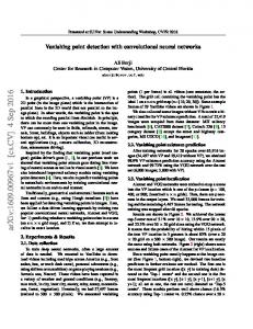
U-net based region detection showed that 99% of the predicted meniscal horn and cartilage bounding boxes match at least 80% of the true bounding box with the actual volume overestimated by about 12%. This overestimation was intentional to ensure the bounding boxes were encapsulating all relevant information to predict the WORMS grading. For the binary meniscus lesion vs. no lesion classifier, specificity of 89.81% and sensitivity of 81.98% were achieved. The corresponding ROC curve including results in training, validation and test sets can be viewed in Figure 2. Areas Under the Curve (AUCs) obtained were 0.95, 0.84 and 0.89 for the 3 sets respectively. In the no lesion class, the distribution of errors between ACL subjects and OA subjects was 43.56% and 56.43% respectively, which reflects the overall distributions of the two groups in the testing set (ACL 40.30% and OA 59.69%). Of the all misclassifications in the no lesion class, 73.26% were made in the posterior horns (45.54% in lateral posterior horn and 27.72% in medial posterior horn) and 26.73% of the errors was made in the anterior horns (19.80% in lateral anterior horn and 6.93% in medial anterior horn). This difference could be due to the imbalanced distribution of lesions in the different horns. For 56.43% of the misclassified cases in the no lesion class, the difference between the two prediction probabilities was higher than 0.9, showing that for these cases the 3D-CNN was not uncertain in assigning the wrong label. For 16.83% of the misclassified cases in the no lesion class, the difference between the two prediction probabilities was lower than 0.1 showing for these cases higher uncertainty in the label assignment. In the lesion class, the distribution of errors between ACL subjects and OA subjects was 51.85% and 48.14% which reflects the overall distributions of the two groups in the testing set in the lesion class (ACL 54.36% and OA 54.36%). Of the all misclassifications in the no lesion class, 96.29% were made in the posterior horns (44.44% in lateral posterior horn and 51.85% in medial posterior horn) and 3.73% of the errors were made in

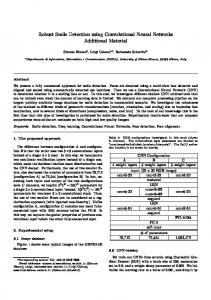
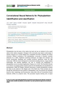
the anterior horns (all in lateral anterior horn). This reflects the distribution of lesion in the four horns in the testing set. For 29.62% of the misclassified cases in the no lesion class, the difference between the two prediction probabilities was higher than 0.9, showing that for these cases the CNN was not uncertain in assigning the wrong label. For 11.11% of the misclassified cases in the no lesion class, the difference between the two prediction probabilities was lower than 0.1 showing a higher uncertainty in label assignment for these cases. The number of cases in this class is too small to assess any distribution between horns of group of subjects in those two groups. For the three class meniscus WORMS model, the best model in terms of classification accuracies was obtained using the ensemble of a 3D neural network with a Random Forest, obtaining accuracies of: 80.74%, 78.02%, and 75.0%, respectively. The count confusion matrix can be viewed in Figure 3. Results of the classification (without considering demographic factors and appending demographics to the 3D-CNN features before the fully connected layer) are reported in Table 3. The big differences observed between training validation and test performance are sign of an overfitting problem, particularly for the “severe” classes. Different hyperparamters and normalization techniques were tried to avoid this overfitting, however we have very small validation and testing sets, particularly for the severe cases (16 in testing), making overfitting difficult to avoid. The binary patellar cartilage lesion vs. no lesion classifier obtained specificity of 80.27% and 80.0%. The ROC can be seen in Figure 4. AUCs obtained were 0.99, 0.86 and 0.88 for the 3 sets respectively. In the no lesion class, the distribution of errors between ACL subjects and OA subjects was 63.56% and 36.44%, which reflects the overall distributions of the two groups in the testing set for the no lesion class (ACL 67.32% and OA 32.68%). For 66.13% of the misclassified

cases in the no lesion class, the difference between the two prediction probabilities was higher than 0.9 showing that for these cases the 3D-CNN was not uncertain in assigning the wrong label. For 12.27% of the misclassified cases in the no lesion class, the difference between the two prediction probabilities was lower than 0.1 showing for these cases higher uncertainty in the label assignment. In the lesion class, the distribution of errors between ACL subjects and OA subjects were 33.51% and 66.49% which reflects the overall distributions of the two groups in the testing set for the no lesion class (ACL 31.42% and OA 68.58%). For 76.12% of the misclassified cases in the no lesion class, the difference between the two prediction probabilities was higher than 0.9 showing that for these cases the CNN was not uncertain in assigning the wrong label. For 9.32% of the misclassified cases in the no lesion class, the difference between the two prediction probabilities was lower than 0.1 showing for these cases higher uncertainty in the label assignment. Model interpretation is challenging considering the complexity of the deep learning pipeline. Even if a shallow classifier is used in the last phase, it is worth noticing that random forests are an ensemble of decision trees chosen on random subsets of the data, which makes it impossible to clearly define which rule the random forest chose. However, we calculated “variable importance” of the random forest and found the importance of the variables to be ranked (from most to least): prediction 1 of the neural network, age, prediction 2 of the neural network, and then gender. While the training of the deep learning pipeline is computationally demanding (70h), the inference on new cases does not require high computational expense. Segmenting the entire knee volume via U-Net takes around 8 seconds, the additional bounding box construction and lesion grading takes about an additional second for a total of ~9 seconds. Inter-rater Comparison

When comparing the selected cases across the 3 different radiologists and the deep learning model, the average agreements between the three experts that performed inter-reader analysis were 86.27% for no meniscus lesion, 66.48% for mild-moderate lesion and 74.66% for severe lesion (Table 4A), while the best deep learning model obtained 80.74%, 78.02% and 75.00% respectively. The average agreements between the three experts that performed inter-reader analysis were 89.56% for no cartilage lesion and 79.74% for cartilage lesion (Table 4A) while specificity and sensitivity of our best binary model were 80.27% and 80.0%. Table 4B reports agreement levels with the grades used for model training. Model Pitfall Evaluation from Musculoskeletal Radiologists For the majority of these cases analyzed, the radiologist agreed that there were features that could make the argument for switching the true grading to the predicted one. Figure 5A shows a case that was graded as having no lesion from the radiologist but the model predicted there was one. There does appear to be small linear signal abnormality (indicated by the red arrow) that may extend to the surface which would classify it as a lesion. Figure 5B shows a case that was graded as having a lesion but the model predicted there was no lesion. This meniscus is severely damaged with significant deformation and irregularity, thus changing the entire shape of the meniscus. For these types of cases, while it is easy for the radiologists to assign the worst grade, the sparsity of similar example in our datasets makes the models’ generalizability to them difficult. Several of the other misclassified cases follow this same pattern; the meniscus was usually severely deformed, which the model likely did not have enough cases to properly learn the numerous variations in which severe meniscus alterations may manifest in severe cases of degeneration. While the three class WORMS model still requires some parameter tuning, it is promising that the

misclassifications generally occur between adjacent groups (i.e. 80% of the no lesion misclassifications are for small lesions). DISCUSSION In this study, we provide a proof of concept of a fully automated deep learning pipeline can identify, with accuracy comparable to the human readers, the presence of OA degenerative morphological features in meniscus and PFJ cartilage. This algorithm has the potential to quickly filter MRIs identifying higher risk cases for the radiologist to further examine. This pipeline also has potential future ability to make more in depth examinations of lesion subjects. With the acquisition of large image repositories such as the Osteoarthritis Initiative database, semi-quantitative scoring systems have been used to grade subjects with OA, and compare lesion severity with other findings such as meniscal defects, the presence of bone marrow lesions, as well as radiographic and clinical scores(21-23). The value of these classification schema has been widely shown in the recent literature(24). In the field of musculoskeletal imaging and specifically in OA, the efforts made in collecting and annotating well-controlled data repositories, such as the OAI, would be best exploited by the translation of artificial intelligence techniques applied to analyze much larger samples. Automation of morphological grading of the tissues in the joint, as proposed in this paper, would be a significant breakthrough in both OA research and clinical practice. It would enable the analysis of large patient cohorts and assist the radiologist/clinician in the grading of images. It would change clinical practice with routine incorporation of semi-quantitative grades in radiology clinical reports. This is a major shift in the paradigm of clinical radiology which could potentially lower the cost in terms of radiologist’s time, and ultimately improve patient outcome.

In this study, we moved in the direction of overcoming this challenge by using concatenation of 2D U-net and 3D CNN for segmentation and lesion detection and severity staging respectively. U-net is a very popular approach for biomedical image segmentation and the application span from 2D (15) to 3D (25-28) and across different modalities and tissues (29,30), showing the flexibility of this model. Applications of 3D-CNN for anomaly detection in MRI are still very limited. While 2D medical image application of deep learning often rely on a simple adaptation of architectures commonly used in computer vision and fine tuning of pre-trained models, the 3-D nature of MRI makes this model inapplicable (11). The relatively small sample size and the large parameter space necessary to span the 3D volume makes the development of 3D-CNNs challenging. While this is the first study exploring the use of 3D convolutional neural network to classify presence or absence of meniscus and cartilage lesion and staging severity in knee MRI, another study with the aim of classifying cartilage lesion using similar MRI knee data and deep learning was recently accepted for publication (31). This method was tested on 175 subjects with a 2D patch-based approach and “hard supervision”, with annotation on presence or absence of cartilage lesion for 2D image patches (64x64) spanning the cartilage region. All the patches were then split in training and testing and no specific information was reported on if this randomization process included constrains to not include different patches of the same subject in both training and test sets. Despite the hard supervision implemented in this study and the relatively homogeneous dataset, the accuracy in binary lesion detection was comparable with what we obtained, sensitivity and specificity equal to 84.1% and 85.2% respectively for evaluation 1 and 80.5% and 87.9% respectively for evaluation 2.

Our model was tested in an almost 10 times bigger and more heterogeneous dataset including OA and ACL subjects before and after reconstruction. We applied a weakly supervised method using annotation on presence or absence of lesions. It was done at the level of the whole volume and not a single patch. By avoiding the needs of annotation on the single image patches, we were able to scale the number of cases, building a more heterogeneous dataset and consequently a more generalizable model. However, it is worth noticing that in our study, results on PFJ cartilage were included while the study from Liu et. al. was performed on TFJ cartilage. Also difference in MRI sequences could affect the results and direct comparison of the performance should be taken in the context of all those differences. Despite the promising results shown in this study, some limitations need to be acknowledged. Even though MRI is considered a sensitive and specific tool for the identification of OA degenerative changes, we still lack an actual gold standard. Previous study reported sensitivity of 91.4 % and specificity of 81.1 % in identifying medial meniscal tears, and of 76 % sensitivity and 93.3 % specificity in identifying lateral meniscal tears (32).

For cartilage lesions, sensitivity and

specificity were reported to be 74.6% and 97.8% (33). The uncertainty in image annotations is a point of great discussion in the field of deep learning applied to medical imaging (34). Recent literature reports examples of applications of Bayesian drop out techniques to model uncertainty applied to neuroimaging (35) and experiments showing the robustness of deep learning to label noise (36). In most of the medical imaging applications there is a lack of a real gold standard and the first aim should be to learn the human behavior, even if it is “imperfect”. While the goal of our study was to train a deep learning model to read images based on how radiologist would interpret images, it could be of interest as a future direction, to use arthroscopy as a standard of reference to fine tune the algorithm. Use of an

external gold standard could be useful to assess if the model is able to over perform the human reading by extracting hidden features in the MRI images that the humans overlook. However, the first step, as presented in this paper, should be to train a model to extract all the features that humans are able to extract, and in a later stage to discover hidden ones. A bigger sample of data annotated multiple times could also be of interest in modeling better the human disagreement specifically studying cases at different level of uncertainty. The neural networks were trained on a single MRI sequence FSE-CUBE acquired in a research setting; larger studies in an uncontrolled environment and using multiple sequences need to be performed to confirm our preliminary observations. Our cartilage model is able to classify the presence or absence of a cartilage lesion in the patella; however, a larger study is needed to generalize this solution on the other cartilage compartments. With the current design we can show a proof of concept of the application of deep learning to the knee MRI inspection and detection of cartilage and meniscus lesion, however, as described in Tiulpin et al. (37), testing of the actual generalizability of our deep learning model would require separate validation on complete different dataset. While this study is too preliminary to make any statement about change of workflow and to comment on directly benefiting patients, it is worth discussing the path we have in vision for these techniques (when mature enough). On a population-basis, the aim will be to automatize the grading process which will allow the analysis of large sample. On a single patient-basis, the usage of objective grades instead of verbal impressions may help in better tracking joint degeneration process. Additionally, the ability of detecting anomaly with an automatic algorithm while the subjects it is still in the scanner could open new possibilities for real time modification of the MRI

protocol to be more precise on the specific needs of the subject, implementing a precision medicine paradigm in the design of MRI protocols. In summary, this study uses deep learning convolutional neural networks to automatically: detect, classify and evaluate OA morphological features. This pilot study reflects a major leap in OA imaging research and represents an important first step in potentially revolutionizing the OA imaging field.

Figures and Tables Legends:

1

64

+ 512

512

256 + 256

128

128

512x512

512x512

512x512

512x512 256x256

512

512x512

256x256

512

256x256 256x256

1024

128x128

32x32

128x128

512

128x128

512

128x128

512

64x64

256

64x64

64x64

256

64x64

64x64

32x32

256

64x64

64x64

128

128x128

128

128x128

256x256

64 128

128x128

256x256

256x256

512x512

512x512

512x512

512x512

for each 2D slice in the MRI volume (248)

512x512x248

128+128 128 128

64

64+64 64 64 11

A 39 x 79 x 44

3 x 3 2D Convolution 39 x 79 x 44

Meniscus Lesion Class {0,1,2}

Age

Gender 5

Transition 2D Max Pooling

28,800

2D Deconvolution/Upsample

24

Flattening

39 x 79 x 44

Concatenation

Random Forest Classifier

Mask Application and Crop 96

B

96

39 x 79 x 44 48

48

24

Flip the column 5 x 5 x 5 3D Convolution 3 x 3 x 3 3D Convolution Fully Connected 4 x 4 x 4 3D Pooling 2 x 2 x 2 3D Pooling

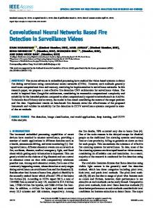
Figure 1: Design of the cascade segmentation and classification model. A) 2D U-Net architecture used for the cartilage and meniscus segmentation (11 class model). Each block represents the 2D slice of the knee MRI volume with corresponding size. The image size shrink in the encoding path of the U-net, due to the application of 3x3 convolutional filters and max puling operations and expand in the decoding path due to deconvolution and up sample operations. The number under each block indicates the number of filters applied at each layer. Arrows that connect encoding and decoding path are called skip connections and they help in preserving from gradient vanishing and to better merge local and global features B) 3D “shallow” CNN for the detection and severity staging of meniscus lesion. The convention used for the architecture visualization is the same as the U-net. The numbers on each box represent the size of the volume at each layer and the number under the box the number of 3D convolutional filters. The features map obtained are flatten in a 1D vector and put as input to a fully connected layer that produce class probabilities. Those probabilistic are than concatenated with demographic factors and used to train a random forest for the final prediction.

Binary Meniscus Lesion Model 1.0

True Positive Rate

0.8

0.6

0.4

0.2

0.0 0.0

Train Train ROC ROC curve curve AUC AUC == 0.99 0.95 Valid Valid ROC ROC curve curve AUC AUC == 0.89 0.84 Test Test ROC ROC curve curveAUC AUC == 0.88 0.89

0.2

0.4

0.6

False Positive Rate

0.8

1.0

Figure 2: Training, Validation and Test ROC curves of the binary meniscus prediction model.

OA Severity Staging Confusion Matrix

Truth Labels

Normal

Mild/Moderate

Severe

Predicted Labels Figure 3: Count confusion matrix of the 3 classes meniscus model in the test dataset.

Binary Cartilage Lesion Model 1.0

True Positive Rate

0.8

0.6

0.4

0.2

0.0 0.0

Train ROC curve AUC = 0.99 Valid ROC curve AUC = 0.89 Test ROC curve AUC = 0.88

0.2

0.4

0.6

False Positive Rate

0.8

1.0

Figure 4: Training, Validation and Test ROC curves of the binary cartilage prediction model.

Figure 5: A) This meniscus was graded as having no lesion but the model predicted there was one. There does appear to be small lesion (indicated by the red arrow) that may extend to the surface which would classify it as a lesion. B) This meniscus was graded as having a lesion but the model predicted there was no lesion. This meniscus is severely damaged and deformed so it was graded as having a complex tear. The sparsity of those cases in the dataset is probably the cause of this error.

TABLES Table 1: Distribution of WORMS grading in the unique 302 subjects ACL unique patients (N=129) Patellar Cartilage Lesion Grade 0 100 (78%) Grade 1 8 (6%) Grade 2 11 (8%) Grade >= 3 10 (7%) Medial Posterior Meniscus Normal 76 (55%) Grade 1 10 (7%) Grade 2 31 (22%) Grade 3 11 (8%) Grade 4 1 (1%) Lateral Posterior Meniscus Normal 65 (50%) Grade 1 11 (9%) Grade 2 39 (30%) Grade 3 12 (9%) Grade 4 2 (2%) Medial Anterior Meniscus Normal 128 (99%) Grade 1 0 (%) Grade 2 0 (0%) Grade 3 1 (1%) Grade 4 0 (0%) Lateral Anterior Meniscus Normal 113 (88%) Grade 1 8 (7.5%) Grade 2 6 (22.5%) Grade 3 1 (5%) Grade 4 1 (7.5%)

OA unique patients (N=173) Patellar Cartilage Lesion Grade (0) 57 (24%) Grade 1 31 (13%) Grade 2 23 (10%) Grade >= 3 62 (47%) Medial Posterior Meniscus Normal 98 (57%) Grade 1 40 (23%) Grade 2 15 (9%) Grade 3 11 (5%) Grade 4 0 (0%) Lateral Posterior Meniscus Normal 123(71%) Grade 1 31 (18%) Grade 2 11 (6%) Grade 3 3 (2%) Grade 4 5 (3%) Medial Anterior Meniscus Normal 166 (96%) Grade 1 2 (1%) Grade 2 2 (1%) Grade 3 2 (1%) Grade 4 1 (1%) Lateral Anterior Meniscus Normal 162 (94%) Grade 1 6 (3%) Grade 2 1 (1%) Grade 3 4 (2%) Grade 4 0 (0%)



Table 2A: Distribution of the meniscus WORMS grades binary classes and severity classes in the training dataset: 1478 subjects (4 horns for each subject N = 5912). mWORMS

0

Description

Normal

Count (%)

4507 (76.23%)

1 Intrasubstance abnormality 735 (12.43%)

2 Nondisplaced tear 373 (6.31%)

3 Displaced or complex tear 192 (3.25%)

4 Disruption and maceration 105 (1.78%)

Binary Classifier

(0,1)

(2,3,4)

Description

Normal

Abnormal

Count (%)

5242 (88.66%)

670 (11.33%)

Severity Classifier

(0,1)

(2,3)

4

Description

Normal

Mild-Moderate

Severe

Count (%)

5242 (88.66%)

565 (9.55%)

105 (1.78%)

Table 2B: Distribution of the patella cartilage WORMS grades and binary classes in the training dataset: N = 1478. mWORMS

0

1

2

Description

Normal

Signal abnormality

Partial thickness defect < 1cm

Count (%)

578 (39.11%)

278 (18.81%)

195 (13.19%)

3 Multiple partial thickness defects 75%

5 Multiple partial thickness defects >1 cm 1 cm >75%

274 (18.54%)

35 (2.37%)

78 (5.28%)

43 (2.91%)

Binary Classifier Description

(0,1)

(2-6)

Normal

Abnormal

Count (%)

856 (57.91%)

622 (42.08%)

6

Table 3: Training, validation and test performances of the 3 classes model: Normal, MildModerate Lesions and Severe Lesions. The table compares the performance obtained by the 3D CNN without the inclusion of demographics, with the inclusion of demographics concatenated with the image based features at the fully connected layer and using the CNN prediction and demographics in an additional shallow classifier. Experiment

3D CNN No Demographics

Class

Normal

MildModerate

Severe

Training

90.24%

96.86%

82.54%

Validation

87.00%

7023%

Testing

87.55%

71.43%

Demographics included in the 3D sCNN

Concatenation of 3D sCNN and Random Forest

MildModerate

Severe

Normal

MildModerate

Severe

94.46%

98.86%

90.48%

80.74%

84.00%

96.80%

37.50%

88.70%

75.00%

43.75%

79.95%

82.10%

75%

66.70%

90.50%

78.00%

66.70%

80.74%

78.02%

75.00%

Normal

Table 4A: Evaluation of the intra-rater variability as comparison with the multi class meniscus and binary cartilage prediction models. Experiment Class

Meniscus intra-rater MildModerate

Normal

Cartilage intra-rater Severe

Normal

Lesions

Expert 1 vs Expert 2 Expert 1 vs Expert 3

85.3% 88.2%

70.6% 76.5%

64.7% 82.4%

80.95% 95.24%

90.00% 76.67%

Expert 2 vs Expert 3

85.3%

52.4%

76.9%

92.50%

72.58%

Table 4B: Comparison with the annotations used for model training. Expert_0 indicated the grading available in our database and performed by one of the 5 radiologists that performed initial grading. Experiment Class Expert 0 vs Expert 1 Expert 0 vs Expert 2 Expert 0 vs Expert 3

Meniscus intra-rater Normal

84.62% 88.46% 88.46%

MildModerate

45.45% 54.55% 54.55%

Cartilage intra-rater Severe

65.00% 55.00% 65.00%

Normal

78.05% 78.05% 97.56%

Lesions

83.61% 86.89% 80.33%

REFERENCES 1.

https://oai.epi-ucsf.org/.

2.

LeCun Y, Bengio Y, Hinton G. Deep learning. Nature 2015;521(7553):436-444.

3.

Ashinsky BG, Bouhrara M, Coletta CE, et al. Predicting early symptomatic osteoarthritis in the human knee using machine learning classification of magnetic resonance images from the Osteoarthritis Initiative. Journal of orthopaedic research : official publication of the Orthopaedic Research Society 2017.

4.

Kim MH, Banerjee S, Park SM, Pathak J. Improving risk prediction for depression via Elastic Net regression - Results from Korea National Health Insurance Services Data. AMIA Annual Symposium proceedings AMIA Symposium 2016;2016:1860-1869.

5.

Liu W, Li Q. An Efficient Elastic Net with Regression Coefficients Method for Variable Selection of Spectrum Data. PloS one 2017;12(2):e0171122.

6.

Caner M, Zhang HH. Adaptive Elastic Net for Generalized Methods of Moments. Journal of business & economic statistics : a publication of the American Statistical Association 2014;32(1):30-47.

7.

Waldmann P, Meszaros G, Gredler B, Fuerst C, Solkner J. Evaluation of the lasso and the elastic net in genome-wide association studies. Frontiers in genetics 2013;4:270.

8.

Ribli D, Horvath A, Unger Z, Pollner P, Csabai I. Detecting and classifying lesions in mammograms with Deep Learning. Scientific reports 2018;8(1):4165.

9.

Becker AS, Bluthgen C, Phi van VD, et al. Detection of tuberculosis patterns in digital photographs of chest X-ray images using Deep Learning: feasibility study. Int J Tuberc Lung Dis 2018;22(3):328-335.

10.

Lee H, Tajmir S, Lee J, et al. Fully Automated Deep Learning System for Bone Age Assessment. Journal of digital imaging 2017;30(4):427-441.

11.

Litjens G, Kooi T, Bejnordi BE, et al. A survey on deep learning in medical image analysis. Medical image analysis 2017;42:60-88.

12.

Kallenberg M, Petersen K, Nielsen M, et al. Unsupervised Deep Learning Applied to Breast Density Segmentation and Mammographic Risk Scoring. Ieee T Med Imaging 2016;35(5):1322-1331.

13.

Lee H, Grosse R, Ranganath R, Ng AY. Unsupervised Learning of Hierarchical Representations

with

Convolutional

Deep

Belief

Networks.

Commun

Acm

2011;54(10):95-103. 14.

Leung MKK, Delong A, Alipanahi B, Frey BJ. Machine Learning in Genomic Medicine: A Review of Computational Problems and Data Sets. P Ieee 2016;104(1):176-197.

15.

Norman B, Pedoia V, Majumdar S. Use of 2D U-Net Convolutional Neural Networks for Automated Cartilage and Meniscus Segmentation of Knee MR Imaging Data to Determine Relaxometry and Morphometry. Radiology 2018:172322.

16.

Chaudhari AS, Fang Z, Kogan F, et al. Super-resolution musculoskeletal MRI using deep learning. Magnetic resonance in medicine 2018.

17.

Liu F, Zhou ZY, Jang H, Samsonov A, Zhao GY, Kijowski R. Deep convolutional neural network and 3D deformable approach for tissue segmentation in musculoskeletal magnetic resonance imaging. Magnetic resonance in medicine 2018;79(4):2379-2391.

18.

Shelhamer E, Long J, Darrell T. Fully Convolutional Networks for Semantic Segmentation. IEEE Trans Pattern Anal Mach Intell 2017;39(4):640-651.

19.

Ronneberger O, Fischer P, Brox T. U-Net: Convolutional Networks for Biomedical Image Segmentation. Medical Image Computing and Computer-Assisted Intervention, Pt Iii 2015;9351:234-241.

20.

Krizhevsky A, Sutskever I, Hinton GE. ImageNet Classification with Deep Convolutional Neural Networks. Commun Acm 2017;60(6):84-90.

21.

Link TM, Steinbach LS, Ghosh S, et al. Osteoarthritis: MR imaging findings in different stages of disease and correlation with clinical findings. Radiology 2003;226(2):373-381.

22.

Felson DT, McLaughlin S, Goggins J, et al. Bone marrow edema and its relation to progression of knee osteoarthritis. Ann Intern Med 2003;139(5 Pt 1):330-336.

23.

Felson DT, Chaisson CE, Hill CL, et al. The association of bone marrow lesions with pain in knee osteoarthritis. Ann Intern Med 2001;134(7):541-549.

24.

Joseph GB, Hou SW, Nardo L, et al. MRI findings associated with development of incident knee pain over 48 months: data from the osteoarthritis initiative. Skeletal radiology 2016;45(5):653-660.

25.

Milletari F, Navab N, Ahmadi SA. V-Net: Fully Convolutional Neural Networks for Volumetric Medical Image Segmentation. Int Conf 3d Vision 2016:565-571.

26.

Roth HR, Oda H, Zhou X, et al. An application of cascaded 3D fully convolutional networks for medical image segmentation. Computerized medical imaging and graphics : the official journal of the Computerized Medical Imaging Society 2018;66:90-99.

27.

Fang L, Zhang L, Nie D, et al. Brain Image Labeling Using Multi-atlas Guided 3D Fully Convolutional Networks. Patch Based Tech Med Imaging (2017) 2017;10530:12-19.

28.

Dolz J, Desrosiers C, Ben Ayed I. 3D fully convolutional networks for subcortical segmentation in MRI: A large-scale study. NeuroImage 2018;170:456-470.

29.

Fechter T, Adebahr S, Baltas D, Ben Ayed I, Desrosiers C, Dolz J. Esophagus segmentation in CT via 3D fully convolutional neural network and random walk. Medical physics 2017;44(12):6341-6352.

30.

Huang L, Xia W, Zhang B, Qiu B, Gao X. MSFCN-multiple supervised fully convolutional networks for the osteosarcoma segmentation of CT images. Computer methods and programs in biomedicine 2017;143:67-74.

31.

Liu F, Z.; Samsonov, A.; Blankenbaker, D.; Larison, W.; Kamarek, A.; Lian, K.; Kambhampati, S.; Kijwiski, R. Deep Learning Approach for Evaluating Knee MR Images: Achieving High Diagnostic Performance for Cartilage Lesion Detection. Radiology 2018; In Press.

32.

Crawford R, Walley G, Bridgman S, Maffulli N. Magnetic resonance imaging versus arthroscopy in the diagnosis of knee pathology, concentrating on meniscal lesions and ACL tears: a systematic review. Br Med Bull 2007;84:5-23.

33.

Kijowski R, Blankenbaker DG, Munoz Del Rio A, Baer GS, Graf BK. Evaluation of the articular cartilage of the knee joint: value of adding a T2 mapping sequence to a routine MR imaging protocol. Radiology 2013;267(2):503-513.

34.

Leibig C, Allken V, Ayhan MS, Berens P, Wahl S. Leveraging uncertainty information from deep neural networks for disease detection. Scientific reports 2017;7(1):17816.

35.

Zhao G, Liu F, Oler JA, Meyerand ME, Kalin NH, Birn RM. Bayesian convolutional neural network based MRI brain extraction on nonhuman primates. NeuroImage 2018;175:32-44.

36.

Rolnick DV, A; Belongie, S; Shavit, N. Deep Learning is Robust to Massive Label Noise. arXiv:170510694v3.

37.

Tiulpin A, Thevenot J, Rahtu E, Lehenkari P, Saarakkala S. Automatic Knee Osteoarthritis Diagnosis from Plain Radiographs: A Deep Learning-Based Approach. Scientific reports 2018;8(1):1727.