Yassine Ben Salem. Mohamed Naceur ABDELKRIM. Electric department, ENIG. Electric department, ENIG. Electric department, ENIG. MACS laboratory.
17th international conference on Sciences and Techniques of Automatic control & computer engineering - STA'2016, Sousse, Tunisia, December 19-21, 2016
STA'2016-PID4115-IFR
3D Face Recognition Using Local Binary Pattern and Grey Level Co-occurrence Matrix Samah YAHIA
Yassine Ben Salem
Electric department, ENIG MACS laboratory Gabès, Tunisia
Mohamed Naceur ABDELKRIM
Electric department, ENIG MACS laboratory Gabès, Tunisia
Abstract—In this paper, we aim to study the problem of 3D face recognition. This problem becomes complex when we consider the human face expressions and different face occlusions. In this context is situated our work, we use the 3D UMB database to evaluate two powerful methods: the 3D Local Binary Pattern (3D-LBP) and the 3D Grey Level Co-occurrence Matrix (3D-GLCM). We tested also the combination of these two approaches. A training phase is necessary, to pass to the test phase which is followed by classification. We use a multiclass Support Vector Machines (SVM) for classification. The experimental results prove that in this classification problem 3DLBP is the more suitable.
we give experiment results obtained and we compare between methods applied. The last section is consecrated for giving conclusions of this study. II. FEATURE EXTRACTION The LBP and GLCM operators, introduced to threat 2D images are the two methods widely used. There are some propositions to extend 2D approaches to analyze 3D texture in different ways. We present in this section the principle of the 2D and some 3D approaches. A. Local Binary Pattern
Keywords— 3D face recognition, classification; 3D-LBP; 3DGLCM; SVM.
1) 2D-LBP operaator x
The basic 2D-LBP operator
The LBP operator, proposed by Ojala [1] consists in dividing image in 3×3 blocs, then compare the center pixel with his neighborhood, if the result of subtraction is positive the pixel is coded by one else it is coded by zero. Finally, a binary number is calculated according to their weights as it shown in Fig 1. Then the histogram obtained from different labels is used as a texture descriptor.
I. INTRODUCTION Facial recognition is becoming more and more a necessity and it’s used in several and diverse areas like airport identification, borders checks, criminal recognition. To be efficient, recognition requires a good analyze of images. 3D images are widely used, it offer more information than 2D images. We find in literature several approaches witch trait 3D volumes such as GLCM, LBP, Gabor filter and Wavelet filter.
ܲെ1
ܲܲܤܮ,ܴ = ݒ(݊݃݅ݏെ ) ܿݒ2ܲ
It is in this context that our work is situated. Since the facial recognition is fragile and complex in that facial expression, or occlusions for example can made a total change of human face. We are interested in this study in a two widely used methods: 3D LBP [4][8][9][14] and 3D GLCM [7][10][11][12][13]. We try to take the advantage that present these methods and test the effect of some changes in human identification. We also evaluate the combination of this to approaches.
(1)
ܲ=0
1, ݔ 0 = )ݔ(݊݃݅ݏቄ (2) 0, < ݔ0 Where Vc and vp represents the values of the center pixel and neighborhood, P corresponds to the number of neighborhood pixels, and R is the radius in pixel.
This paper is organized as follows: we present in Section 2 the principle of LBP and GLCM approaches with the extension to the third dimension. Then, we describe our works and explain different steps of our study in section 3. Finally,
978-1-5090-3407-9/16/$31.00 ©2016 IEEE
Electric department, ENIG MACS laboratory Gabès, Tunisia
51
40
45
1
22
50
39
0
31
52
53 Thresholding 0
0
0 0
1
1
(00110001)2=25
Encoding
Figure1. Example of 2D-LBP calculation
328
“Uniform patterns” are an extension of the original LBP. A uniform pattern contains at most two bitwise transitions from 1 to 0 or vice versa. LBP is extended by defining circular neighborhoods with different number of pixels [5].
Vq : the result of subtraction. q : index of value in volume V P: number of points in circle R : rayon of circle
2) The 3D-LBP operator x
V: the volume pixel
LBP –TOP (Local Binary Pattern histograms from Three Orthogonal Planes)
L: interval of time (or the z axe) The volume is segmented in three parallel planes; from these planes the co-occurrences of all neighboring points are extracted.
This proposition consist in segmenting the image in three orthogonal planes 2D (XY , XT and Y T ). Planes intersected in a center pixel as demonstrate Fig 2. In each plane the LBP 2D is calculated and thus three histograms are created denoted as XY-LBP, XT-LBP and YT-LBP.
An example is found in [9] present an example of VLBP with the z axe: L is equal to 1, the number of points P is equal to 4 and the rayon R is equal to 1.
Finally, histograms obtained are concatenated into one histogram which represent the description of the all 3D image [4][8][14]. We note that the number of neighboring points PXY, PXT , PYT in the XY , XT and YT planes can be different and the radii in axes X, Y and T RX, RY and RT can also be changed. The corresponding LBP-TOP feature became LBP í T OP PXY ,PXT ,PY T ,RX,RY ,RT .
Figure 3. Example of V LBP1,4,1 .calculation[9]
B. Grey Level Co-occurrence Matrix
Figure 2. Example of LBP-TOP calculation [8]
x
1) The 2D-GLCM x
VLBP (Volume Local Binary Pattern)
This method proposed by Haralick in 1973 [2], is based on the calculation of the co-occurrence matrix which is nconstructed by calculating the number of repetition of each pair (i,j) separated by a distance d = (dx, dy), and according to D� GLUHFWLRQ� ș (0°, 45°, 90°, and 135°), the position angle between two pixels. The offset parameter affects the GLCM features vector is defined as: offset= (0 d, -d d,-d 0, -d –d).The co-occurrence matrix is computed using this equation:
This proposition is based on a volume V which is composed of neighbor’s points of image slices, and defined by: [9] ܸ = ݒ(ݒ0 , … ݍݒ, … ݒ3+1 )
(3)
The LBP code is calculated using this formula: 3ܲ+1 ܸܮܲܤܮ,ܲ,ܴ = σ=ݍ0 ݍݒ2ݍ
The basic 2D-GLCM
(4)
With:
3��
݀ܥ,ߠ (݅, ݆) ݔ
ݕ
1 ݂݅ ݂(ݔ, ݔ(݂ ݀݊ܽ ݅ = )ݕ+ ݀ݔ, ݕ+ ݆݀ = )ݕ = ቄ 0 ݁ݏ݅ݓݎ݄݁ݐ
(5)
=ݔ1 =ݕ1
In order to determinate the similarity between different GLCM Haralick’s proposed 14 statistical features. This statistical features are calculated to represent the characterizations of the image texture [2][5][6]. The four principle features are the Angular Second Moment, the entropy, the correlation and the contrast defined as: -
The Energy or Angular Second Moment N �1 N �1
¦¦ C
ASM
2 mn
m 0n 0
-
The Entropy
ENT -
Figure 4. Volumetric GLCM [10]
N �1N �1
C ¦ ¦ 1 � mmn� n m 0n 0
(7)
x
The Correlation
COR
N �1 N �1
¦¦
(1 � P x )(1 � P y )
m 0n 0
-
(6)
The Contrast
CON
V xV y
C mn (8)
N �1N �1
¦ ¦ (m � n) 2 .Cmn
m 0n 0
(9)
Volumetric GLCM (VGLCM)
Proposed by Tsai in 2007 [13], the idea is to threat 3D data as an image cube using the volumetric characteristics. If we note n the number of grey level and d=(dx,dy,dz) the moving box, the co-occurrence matrix, it is an n-by-n matrix and is defined by: ݅(ܥ, ݆) = 1 ݂݅ ݂(ݔ, ݕ, ݅ = )ݖ σ=ݔݔ1 σ= ݕݕ1 σ=ݕݕ1 ൝ܽ݊݀ ݂( ݔ+ ݀ݔ, ݕ+ ݀ݕ, ݖ+ ݆݀ = )ݖ 0 ݁ݏ݅ݓݎ݄݁ݐ
The 3D-GLCM detailed in [12] is an expanded approach from the original 2D-GLCM. It consist in calculation of triplet (i,j,k) grey level repetition instated of pairs (i,j). As the same manner as in 2D-GLCM, the triplet (i,j,k) of grey level are separated by a distance d and follow D� GLUHFWLRQ� ș. Consequently, co-occurrence matrix is an n-by-n-by-n matrix as it shown in Fig. 5, and described in the following equation: ݅(ܥ, ݆, ݇, ݀, ߠ) max(|݊ݔ1 െ ݊ݔ2 |, |݊ݕ1 െ ݊ݕ2 |) = ݀ max(|݊ݔ2 െ ݊ݔ3 |, |݊ݕ2 െ ݊ݕ3 |) = ݀ ተ ȣ൫(݊ݔ1 , ݊ݕ1 ), (݊ݔ3 , ݊ݕ3 )൯ = ߠ ൫(݊ݔ1 , ݊ݕ1 ), (݊ݔ2 , ݊ݕ2 ), (݊ݔ3 , ݊ݕ3 )൯ ං (11) = ܰൾ ܯ א1 ܯ כ2 ܯ כ3 I(݊ݔ1 , ݊ݕ1 ) = ݅ ተ I(݊ݔ2 , ݊ݕ2 ) = ݆ I(݊ݔ3 , ݊ݕ3 ) = ݇
2) The 3D-GLCM operator x
3D- GLCM
We note that n1 and n2 represent respectively the first and the second neighbor.
(10)
It consist in computing two pixels C(x, y, z) and C(x+dx, y+dy, z+dz), which are equal to i and j, within a moving box. Each pixel has 27 neighbors and move in 13 directions [7][10][11][13]. To speed up the calculation, cubes are segmented in some windows as it shown in Fig 4, and to each window the cooccurrence matrix is defined.
Figure 5. Presentation
Once 3D GLCM has been calculated, as in 2D Haralick’s textural features can be computed from these matrixes as previously defined in (6) ,(7) ,(8) and (9) [10].
33�
of the 3D-GLCM [12]
III. WORK DESCRIPTION I.
Description of our work
In this section, we present the UMB database, the database used for experiments, and we describe the phase of realization of these experiments.
Image training
Image classifying
3D Image to train
3D Image to classify
Pretreatment A. The University of Milano Bicocca 3D face database The University of Milano Bicocca 3D face database (UMBDB) [3] contains 143 subjects (98 male and 45 female). Images taken include occlusions such as scarves, telephone, eyeglasses and some facial expressions. It is a rich database.
3D method application
Features extraction
The occlusions in this database are difficult and can be caused by eyeglasses, hands, hats, scarves, hair and other objects. Moreover, the amount and the locations of occlusions change greatly. The figure 6 illustrates examples of facial expressions (smile, angry, neuter and boring) and the figure 7 presents some examples of occlusions that can be found in the UMB database (scarves hat and bottle).
Training phase
Pretreatment
3D method application Features extraction
Classification phase
Classification result Figure 8. The classification algorithm.
-
Training and test step: consist in selecting some simples representing the different classes and calculating a 3D recognition method. After a pretreatment (adjusting resizing and converting each image to the grey level scale), we have applied the recognition method, and then we have extracted features. Thus each image is defined by a vector of parameters. When we have calculated the cooccurrence matrix, the parameters of vector are the four parameters extracted contrast, correlation, energy and homogeneity. When we have applyed the LBP, histograms are used as parameters in the vector. The test step consists in testing the 3D recognition method on simples of classes.
-
The classification step: the aim of this step is to assign to each image the corresponding class. We have chosen in this for classification the multi-class support vector machine (SVM). This classifier is powerful and rapid. It is based on the calculation of a function or hyper plane, which separates classes [5]. This hyperplane separates classes of input data points (Fig 9). M is the margin or the distance from the hyperplane to the closest point for both classes of data points.
IV. EXPERMINENTAL RESULT Figure 6. Examples of facial expressions in the UMB database
Figure 7.Examples of occlusions in the UMB database
B. Phase of experiments We have performed two experiments using the proposed database in the aim of comparing the performance of the used methods. Basing on the variety of images taken in the UMB database, we have chosen to study the problem of face identification with two ways: in experiment 1 we have considered some facial expressions (smile, angry, neuter, boring) and in experiment 2 we have considered both facial expression and some occlusions (scarves hat, eyeglasses...). Our work can be resumed as it shown in Fig 8. It consisted primarily in two main steps: training and classification. The texture classification phase is based on the comparison of two features vectors. The train features vector is obtained by applying a recognition method. For each sample, the test features vectors are calculated using the same method.
33�
We have satisfied by calculating for basic features: energy, correlation, homogeneity and contrast. The rest of features didn’t ameliorate the classification. Results obtained in this experiment are summarized in the table 1. TABLE 1 Comparison of simulation results obtained in experiment 1 3D-LBP
3D-GLCM
3D-LBP +3D-GLCM
93.13%
65.63%
86.25%
B. Experiment 2 The same work as experiment 1 is done, we have tested the same algorithms as the same manner; just here we have considered with both some facial expression some occlusions. Since occlusions founded in the UMB database are very different, facial identification in this case becomes more complex. To do this, we have tested the algorithms with 18 classes; each class contains 8 samples, 54 train samples and 144 test samples. Results are presented in the table 2:
Figure 9. classification with the Support Vector Machine classifier
V. EXPERIMENT RESULT A. Experiment 1 The aim of this experiment is to evaluate 3D-LBP and 3DGLCM approach in face recognition. A percentage of the successful classified images have been calculated.
TABLE 2 Comparison of simulation results obtained in experiment 2
We have considered different facial expressions (neuter, smile, angry and boring). We have tested the algorithms with 32 classes; each class contains 5 samples, 64 train samples and 160 test samples.
3D-LBP
3D-GLCM
3D-LBP +3D-GLCM
88.88%
57.63%
83.33%
We note that results of classification in experiment 2 are less than these obtained in experiment1. This explained that in experiment 2 we have taking in consideration some and different occlusions with some faces expressions, the problem of face recognition became more difficult.
We have used the two methods for the features extraction phase: 3d-LBP, 3D-GLCM and the fusion of the methods, LBP+GLCM. The combination of 3D-LBP and 3D-GLCM consist in applying the LBP operator on the co-occurrence matrix. That’s mean we have calculated the co-occurrence matrix for three planes then in this matrixes, we have extracted the LBP pattern instead of features defined in (6), (7), (8), and (9).
VI. CONCLUSION In this study, we have extracted three kind of texture features based on the 3D-LBP, the 3D-GLCM, and the combination of 3D-LBP and 3D-GLCM for face recognition. The classification experiment was done using the UMB database. SVM was adopted to train and test different texture feature extracted.
We have modeled textures with VLBP [9] so 3D images have been segmented on three planes and to each plane the approach 2D has been applied and features have been extracted. Results obtained from different planes have been concatenated.
We conclude from our experiments that the 3D-LBP method gives the best result of classification comparing to the 3D-GLCM. Even if combine the two methods, results did not be ameliorated. So, it’s clearly that the 3D-LBP is more suitable for treatment of face recognition problems. Besides, our study highlighted the performance of SVM classifier; it’s a powerful and simple algorithm. This study proves that human identification steel a complex problem and require test not only powerful algorithms but several test to decide which the successful approaches is.
The best results are obtained by the 3D-LBP and after varying the parameters of this approaches (Z axe, number of points, rayon) as this manner: (1,8,1), (1,8,2), (1,8,3) and (1,16,1), with an offset equal to (0,1,0). The 3D-LBP has been calculated with these four parameters. The feature vector is composed by the four patterns concatenated. Concerning 3D-GLCM, we have applied the Volumetric GLCM [10]. 3D images have been segmented in three windows and in each window the 2D co-occurrence matrix has been computed. The best averages have been estimated when we have varied the two parameters (offset and Numlevels) with the couple the horizontal position ș� �0°, offset = (0, 1, 0)
In the future work, we will ameliorate classification results by associating with face another biometric technique like finger print or iris. We will also try to extract features from other popular methods.
33�
REFERENCES [1]
[2]
[3]
[4]
[5]
[6]
[7]
[8]
Ojala, T., M. Pietikäinen, and T. Mäenpää. “Multiresolution Gray-Scale and Rotation Invariant Texture Classification with Local Binary Patterns”, IEEE Transactions on Pattern Analysis and Machine Intelligence, vol. 24 (7), 971-987. Haralick, R. M., Shanmugam, K., Dinstein, I.”Textural features for image classification”. IEEE Trans. Systems. Man. Cybernetics. 3(6), 610-621. A. Colombo, C. Cusano, and R. Schettini. “The University of Milano Bicocca 3D face database.” University of Milano Bicocca. 2011. url: http://www.ivl.disco.unimib.it/umbdb/index.html. Xiaohong W. Gao, Yu Qian and Rui Hui.The. “Rotation Invariant Image and Video Description with Local Binary Pattern Features” IEEE TRANSACTIONS ON IMAGE PROCESSING, 2010 Yassine Ben Salem, Salem Nasri. “Rotation Invariant Texture Classification using Support Vector Machines.” Communications, Computing and Control Applications (CCCA), 2011 International Conference. . Haralick, R. M., Shanmugam, K., Dinstein. “On some quickly computable features for texture” IEEE transaction on system, man and cybernetic november 1973 Baladhandapani Arunadevi and Subramaniam.”BRAIN TUMOR TISSUE CATEGORIZATION IN 3D MAGNETIC RESONANCE IMAGES USING IMPROVED PSO FOR EXTREME LEARNING MACHINE”. N. Deepa Progress In Electromagnetics Research B, Vol. 49, 31–54, 2013 Che-Wei Chang, Chien-Chang Ho and Jyh-Horng Chen. “ADHD classification by a texture analysis of anatomical brain MRI data” Frontiers in Systems Neuroscience September 2012 Volume 6 Article 66
[9]
Guoying Zhao and Matti Pietikäinen “Dynamic Texture Recognition Using Volume Local Binary Patterns Machine Vision Group”. IEEE TRANSACTIONS ON PATTERN
ANALYSIS AND MACHINE INTELLIGENCE, 2007
[10] Andrés Ortiz, Antonio A. Palacio, Juan M. Górriz, Javier Ramírez, Diego Salas-González. “Segmentation of Brain MRI Using SOM-FCMBased Method and 3D Statistical Descriptors” ARTICLE in COMPUTATIONAL AND MATHEMATICAL METHODS IN MEDICINE · MAY 2013 [11] C. Eichkitz, J. Amtmann & M.G. Schreilechner. “Application of GLCMbased Seismic Attributes forAnisotropy Detection” 76th EAGE Conference & Exhibition 2014 Amsterdam RAI, The Netherlands, 16-19 June 2014 [12] Wen-Shiung Chen, Ren-Hung Huang, and Lili Hsieh. “ Iris Recognition Using 3D Co-occurrence Matrix. ̌M. Tistarelli and M.S. Nixon (Eds.): ICB 2009, LNCS 5558, pp. 1122–1131, 2009. [13] Fuan Tsai, Chun-Kai Chang, Jian-Yeo Rau, Tang-Huang Lin, and GinRon Liu “3D Computation of Gray Level Co-occurrence in Hyperspectral Image Cubes”. A.L. Yuille et al. (Eds.): EMMCVPR 2007, LNCS 4679, pp. 429–440, 2007.
[14] Xiaohong Gao, Yu Qian, Martin Loomes, Richard Comley,
Balbir Barn, Alex Chapman, Janet Rix, Rui Hui, Zengmin Tian. “Retrieval of 3D Medical Images via Their Texture Features”. International Journal on Advances in Software, vol 4 no 3 & 4, year 2011, http://www.iariajournals.org/software/
33�