As an illustration of this procedure, a new prototype 3D ... popular 3D sensors is done in Sec. III, which ..... A recent tutorial in [13] covers many aspects of sensor.
final version in: International Conference on Intelligent Robots and Systems (IROS), IEEE Press, 2007
3D Forward Sensor Modeling and Application to Occupancy Grid based Sensor Fusion Kaustubh Pathak, Andreas Birk, Jann Poppinga, and S¨oren Schwertfeger Abstract— This paper presents a new technique for the update of a probabilistic spatial occupancy grid map using a forward sensor model. Unlike currently popular inverse sensor models, forward sensor models can be found experimentally and can represent sensor characteristics better. The formulation is applicable to both 2D and 3D range sensors and does not have some of the theoretical and practical problems associated with the current approaches which use forward models. As an illustration of this procedure, a new prototype 3D forward sensor model is derived using a beam represented as a spherical sector. Furthermore, this model is used for fusion of point-clouds obtained from different 3D sensors, in particular, time-of-flight sensors (Swiss-ranger, laser range finders), and stereo vision cameras. Several techniques are described for an efficient data-structure representation and implementation. The range beams from different sensors are fused in a common local Cartesian occupancy map. Experimental results of this fusion are presented and evaluated using Hough-transform performed on the grid.
I. I NTRODUCTION Mobile robot based mapping using occupancy grids is a widely used method at present [1], [2]. The aim of this paper is to come up with a scheme of map update which allows for easy incorporation of a given sensor’s physical characteristics. Not only is the resulting map more accurate, but it also can be fused more systematically with another map generated using a sensor based on an entirely different operating principle. This applies in particular to the variety of 3D sensors currently in use. Sec. I-A introduces the basic terminology. The current state of the art and its shortcomings are touched upon in Sec. I-B. The novel scheme for reformulation of forward sensor model and its corresponding update equations are presented in Sec. II. Application of this scheme to currently popular 3D sensors is done in Sec. III, which includes a general sensor model formulation and grid based sensor fusion. Efficiency issues of implementation are covered in Sec. IV. Sec. III presents some experimental results, followed by conclusion. A. Basic Terminology and Formulation In the occupancy grid paradigm, the state to be estimated consists of a discrete map which is a collection of cells G , [mi ], i = 1 . . . Nmap , each of which can be occupied mi = 1, or unoccupied mi = 0. This state-space is binary and also static for a given robot location and orientation. This work was supported by the German Research Foundation (DFG). The authors are with the Dept. of Electrical Engineering and Computer Science, Jacobs University Bremen, 28751 Bremen, Germany.
(k.pathak, a.birk)@jacobs-university.de
Z
r
φ X
θ rxy
Fig. 1. Spatial beam parameterization. rxy refers to the beam’s projection on the XY plane.
Therefore, it is commonly estimated directly using the binary static version of the Bayes filter [3]. The probability that a particular cell is occupied is p(mi = 1) ≡ p(mi ). The probability that the cell is unoccupied is p(mi = 0) ≡ p(¬mi ) ≡ 1−p(mi ). We write vectors and lists in bold. Therefore, p(m) ≡ [p(mi )]. In this paper, we use only probability mass functions (pmf’s), also called discrete probability distribution functions (d-pdf’s). ˆk | Each sensor observation is a list Z = [rk = rk ρ k = 1 . . . Nbeams ] of the range rk along various lines-ofˆk. A sight (LOS) directions (beams) denoted by unit vectors ρ general beam, as shown in Fig. I, would be denoted without the subscript as r = rˆ ρ. Each such beam carries information about only a list m(r) = [mi | i = 1 . . . Ncells ] of cells, and m(r) ⊆ G. The parameter Ncells would be different for different beams. The list m(r) is arranged in ascending order of the distance to the sensor. We recall some standard definitions [1]. The conditional probability p(rk | mi ) is called the forward sensor model. It gives the probability of observing a reading rk , when the state of the ith cell is mi . Similarly, p(mi | rk ) is the inverse sensor model, since it goes from effects (rk ) to causes (mi ). Forward models have the advantage that they can be easily determined experimentally and can characterize a sensor in a more straightforward manner. A classical forward beam model applicable to laser range finders (LRFs) is given in [1] and plotted in Fig. 2(a). B. Popular Cell-update Approaches and their Disadvantages Let us consider a list of cells m(r) along a beam. Elfes [4] assumed that the occupancy probability of each cell in the grid is independent of the other. We make the same
assumption and proceed as in [3]. p(mi ) already reflects the information in the last sample r− at time instant t − 1. We now wish to update p(mi ) using the new sample r+ at time instant t. The sensor samples are also considered independent of each other, so p (r+ | mi ∧ r− ) = p (r+ | mi ). From Bayes theorem, we get p(mi | r+ ∧ r− ) = p(r+ | mi )p(mi | r− ) p(r+ | mi )p(mi | r− ) + p(r+ | ¬mi )p(¬mi | r− )
II. R EDEFINING F ORWARD S ENSOR B EAM M ODEL A. A Cell Occupancy Probability Mapping
(1)
One current approach is to compute the forward model p (r+ | mi = 1) using a formalism such as that given in [1]. This model has two disadvantages: Firstly, it inherently assumes that the beam-range r returned by a sensor when cell mi is occupied is not influenced by the occupancy state of other cells. This is not true because if a cell mj , j < i is occupied, it will short circuit mi so that p(r | mi = 1) → 0. The model attempts to partially heuristically rectify this by having an exponentially decreasing term. Secondly, (1) has the term p(r+ | ¬mi ) 6= 1 − p(r+ | mi ).
One of the main contributions of this paper is to come up with a modified definition of sensor forward model and a systematic scheme for beam cell-probability update which does not have the disadvantages noted in the other approaches noted in this section.
(2)
This term is quite difficult to interpret and compute in practise. This issue seems to be mostly unaddressed in the literature. Another approach suggested in [5] would be to consider all possible permutations of cell occupancies X (mi ) = [m1 , . . . , mi-1 , mi+1 , . . . , mNcells ] , mj = 0/1, as follows X p(r+ | mi ) = p(r+ | mi ∧ X (mi ))p (X (mi ) | mi ) . X (mi )
There are 2Ncells −1 such permutations and it is computationally expensive to use this definition. In both of the above approaches, the authors finally resort to using a reverse sensor model by reformulating (1) to get p (mi | r+ ) p (¬mi ) p (mi | r− ) p (mi | r+ ∧ r− ) = p (¬mi | r+ ∧ r− ) p (¬mi | r+ ) p (mi ) p (¬mi | r− ) (3) This has the advantage that hard to compute terms like (2) cancel out. However, it loses the ability to use a forward sensor model which can be experimentally found. Finding an inverse sensor model is difficult: refer to [1] for a neuralnetwork based method for estimating a sensor reverse model. A third approach used by [2, Eqs. (8,9,10)] is to use the following formula, where p¯(x) ≡ 1 − p(x). � p mi | r+ ∧ r− = p (r+ | mi ) p (mi | r− ) (4) p(r+ | mi )p(mi | r− ) + p¯(r+ | mi )¯ p(mi | r− ) On comparing this with (1) and noting (2), it can be concluded that (4) is incorrect. Finally, the approach of Thrun [6] which uses forward models employs a time-consuming iterative ExpectationMaximization (EM). Furthermore, it was designed for application to wide beam-cone sensors like the SONAR.
We present here an alternate definition of the sensor forward model, partially based on [4]. Instead of dealing directly with the cell occupancy probabilities, we introduce intermediate variables Bi , i = 1 . . . Ncells + 1 whose probabilities have a one-to-one nonlinear mapping RNcells +1 → RNcells to those of the cells’ occupancy. These variables are analogous to the correspondence variables of [6]: however, unlike that work, our approach does not require EM iterations for cell occupancy updates. Definition 2.1 (Bi ): For a list m(r) of cells, Bi is defined as the event that the cell mi is occupied but all cells before it are unoccupied. The state of the cells after the ith cell is irrelevant. 1 Bi , 000 . . 000} |{z} | .{z
xxx . . xxx} | .{z
(5)
i − 1 free cells. mi = 1 Short-circuited cells.
In this formulation, i = 1 . . . Ncells + 1 and BNcells +1 ≡ 000 . . . 000, i.e. the event that all cells are unoccupied. We define the operator kBi k to return the radial distance of the center of the cell mi from the sensor origin. This is the range an ideal sensor will return if p(Bi ) = 1. / The events Bi , i = 1 . . . Ncells + 1 have the following properties. 1) They are exhaustive and mutually exclusive. Therefore, their probabilities p(Bi ) are such that p(
Ncells [+1
Bi ) =
Ncells X+1
i=1
p(Bi )
= 1.
(6)
i=1
2) The occupancies of all the cells are assumed to be independent of each other. This means that pi6=j (mi ∧ mj ) = p(mi )p(mj ). The probabilities p(Bi ) have a one-to-one relationship with the cell occupancy probabilities p(mi ). This can be stated as p(Bi ) = p(mi )
i−1 Y
p(¬mj ), i = 1 . . . Ncells ,
j=1
p(BNcells +1 ) =
N cells Y
p(¬mj ).
(7)
j=1
3) Note that the event Bi does not contain any information about the occupancy status of the cells mj , j > i. This can be seen when we invert (7). After performing some algebra, one gets −1 i−1 X p(mi ) = p(Bi ) 1 − p(Bj ) . (8) j=1
If a denominator number k in Eqs. (8) vanishes, all the subsequent ones vanish also. This means that there is no information in the list p(B) about the probabilities of those cell numbers i > k, and they are unaffected. This is another advantage of using the intermediate variables Bi .
TABLE I C OMPARISON OF 3D S ENSORS Information Manufacturer Range [rmin , rmax ] Horiz. FOV Vert. FOV Resolution
Swiss Ranger CSEM [600, 7500] mm 47o 39o 176 × 144
Stereo Camera Videre Design [686, ∞] mm 65.5o 51.5o 640 × 480
B. Modified Forward Sensor Beam Model
p(r ∈ D | Bi ),
i = 1 . . . Ncells + 1.
(9)
350
Stereo Cam Linear Fit Swiss Ranger
35 30
150
σ(r) (mm)
250 200
25 20 15
100 10 50
Conveniently enough, we can still use some of the classical beam models like the one described in [1]. We would just need to reinterpret p(r | mi = 1) to mean p(r | Bi ). What has changed, however, is that we cannot update the cell probabilities the old way. This is shown next.
Stereo Cam (SC) Swiss Ranger SC Theoretical Quadratic Fit
40
300 Error= µ(r) − rn (mm)
In light of the reasons outlined in Sec. I-B, our motivation for the definitions of events B in Sec. II-A becomes clear, namely, that they are exhaustive and mutually-exclusive, and that they capture the state of all the cells in the beam at a time. In terms of these new variables, the forward sensor beam model may be written as a pmf defined on the discrete set D , {kBj kˆ ρ | j = 1 . . . Ncells }.
1000 2000 3000 Nominal Ground Truth Range rn (mm)
5 1000
2000 rn (mm)
3000
Fig. 3. Comparing the error in the means value µ(r) and the standard deviation σ(r) of the Swiss Ranger(SR) vs. the Stereo Cam(SC). Refer to Table II for the polynomials fitted on this data.
C. Beam Occupancy Probability Update The event space B is not binary but has Ncells + 1 members. Therefore, the cell probability update equation is now different. When we want to update the occupancy probabilities of cells ∈ m(r+ ) along a new sensor sample r+ , given the previously computed values p(mi | r− ), we need the following steps. 1) Compute p(Bi | r− ∈ D), i = 1 . . . Ncells + 1 by substituting p(mj | r− ), 1 . . . Ncells in the RHS of Eq. (7). If we have a predefined number of beams, the values p(Bi ) can be cached, making this entire step unnecessary. In this case, p(mj | r− ) will already be consistent. 2) Apply Bayes theorem to compute the new values p(Bi | r+ ∈ D) as follows ∀i = 1 . . . Ncells + 1 p(r+ | Bi ) p(Bi | r− ) (10) p(Bi | r+ ) = PNcells +1 p(r+ | Bj ) p(Bj | r− ) j=1 = ηB p(r+ | Bi ) p(Bi | r− ).
(11)
Here, ηB is the normalizer and p(r+ | Bi ) is the sensor forward beam model as mentioned in (9). Note that p(Bi | r+ ) already satisfy (6). This update step requires Ncells + 1 forward model evaluations per cell update (followed by Ncells evaluations of (8)). Eq. (11) is important because it lets us apply an occupancy update directly on p(Bi ) using a forward model without needing the difficult to calculate terms like in (2). 3) Compute p(mj | r+ ) from p(Bi | r+ ) using Eq. (8). As already mentioned, depending on the actual values of p(Bi | r+ ) some cell probabilities may remain unchanged because no new information concerning them is contained in the new sample.
These steps are repeated recursively at each time instant for each beam returned by the sensor. This procedure has none of the disadvantages of the approaches mentioned in Sec. I-B. On applying Eq. (11) to the classic beam model of Fig. 2(a), one obtains the graphs shown in Figs. 2. III. A PPLICATION TO 3D S ENSORS To motivate the empirical derivation of the 3D sensor models to be presented subsequently, we take a brief digression to introduce two 3D sensors being used in our robotics lab. There are several options for 3D data acquisition like 3D laser scanners [7], [8], [9] or stereo cameras [10], [4]. In our experiments, a time-of-flight based SwissRanger SR-3000 [11] and a Stereo camera Stereo-on-Chip (STOC) [12] were used. Their locations on the robot are indicated in Fig. 5(a). The technical details of these sensors are summarized in Table I. Their relative accuracy is compared in Fig. 3. As described in [12], the range-resolution ∆r of a stereo-camera is proportional to the square of the range and has a systematic error in the mean error which is linear with respect to the range. Refer to Fig. 3 for a comparison of this dependence with the experimental observations. The Swiss-ranger shows a similar decay but to a lesser degree. Good forward sensor models of stereo cams are hard to come by [10]. A. Forward Beam Modeling for 3D Sensors In this section, we restrict ourselves to the 3D sensors already mentioned in Sec. III, viz. the Swiss ranger and the stereo camera. Remark 3.1 (3D Sensors Characteristics): Experimental readings as shown in Fig. 3 show that the beam model as
p(r | m11=1)
0.15
0.1
0.05
0 0
0.5 Range r
1
(a) The classical beam forward model p(r|m11 = 1), kB11 k = 0.5 [1].
Fig. 2.
(b) Updating the distribution p(Bi | r) 20-times for the same sensor sample r = 0.5. We start from an assumption that nothing is known about the cell occupancy. After the iterations, we see a clear accumulation of probability at kBi k = 0.5.
Application of Eq. (11) to the classic beam model shown in Fig. 2(a). Note that the time-step axis increases towards the front.
TABLE II 2 +a r +a . C ORRECTION POLYNOMIALS q(rn ) = a2 rn 1 n 0 sr qµ sc qµ sr qσ sc qσ
(c) Updating the distribution p(mi | r) 20-times for the same sensor sample r = 0.5 using Eq. (8) and the values in Fig. 2(b). Note that we start from a uniform cell occupancy probability of 0.5.
a2 . 0.0 0.0 −0.243897 × 10⁻⁶ 0.947909 × 10⁻⁵
a1 . 1.0 1.150204 0.486625 × 10⁻² −0.178817 × 10⁻¹
a0 . 0.0 −78.158607 −0.7691149 11.186380
in Fig. 2(a) is not entirely valid for commonly used 3D sensors. The main differences are as follows. Both the sensors are not able to detect any obstacles with range less than rmin . This means that the Pforward model p(r | Bi ) is not exhaustive, meaning that r∈D p(r | Bi )dr = 0, if kBi k < rmin , where, kBi k is defined in Def. 2.1 and the set D was defined before Eq. (9). The false beams reporting maximum range as found in the classical model seem to be mostly absent from the given 3D sensors’ samples. In their place, we now have to deal with false negatives, i.e., cases where the sensor does not report an obstacle even when one P is present within the maximum range. This implies that r∈D p(r | Bi )dr < 1, if rmin ≤ kBi k ≤ rmax , This again shows that the model is not exhaustive even when rmin ≤ kBi k ≤ rmax . As illustrated in Fig. 3, the standard deviation σ is a function of the ground-truth nominal range rn . This effect is more pronounced for the stereo camera. This function can be approximated by a polynomial qσ (rn ). Refer to Table II. As is clear from Fig. 3, the stereo camera has a systematic linear degradation of the mean accuracy with the range. This function too can be approximated by a polynomial qµ (rn ). Refer to Table II. Although the theoretical maximum range for the Swissranger SR3000 is quite large and that of the stereo camera STOC is unlimited (Table I), we restrict it to a finite value rmax for practical computational purposes. We note that rmax can be chosen to be the maximum kBNcells k among all the beams considered. A sensor range sample of r > rmax carries information which should not be discarded. It shows that all cells along that beam are probably free. This case shows another advantage of our reformulation of the sensor forward model,
namely, that we have an explicit event BNcells +1 which handles it. Extending (9), we could say that for i = 1 . . . Ncells , p(r ∧ r > rmax | Bi ) ≡ 0.
(12)
p(r ∈ D | BNcells +1 ) ≡ �,
(13)
p(r ∧ r > rmax | BNcells +1 ) ≡ 1 − �.
(14)
Here, 1 � � > 0 is a small value found experimentally. / We now formulate a forward 3D sensor model which is inspired by their above mentioned characteristics. Definition 3.1 (Normal Probability Mass Distribution): ) ( 2 (r − kB k) 1 i (15) N (r ∈ D, kBi k, σ 2 ) , √ exp − 2σ 2 σ 2π We recall that the normal distribution has most of its probability (99.73%) within µ ± ∆σ, ∆ = 3. / Finally, Algorithm III.1 gives the resulting general 3D sensor forward model p(r ∈ D | Bi ) defined by using the polynomial definitions in Table II.
Algorithm III.1: p(r | Bi ) µi ← qµ (kBi k), σi ← qσ (kBi k) rlimit ← qµ (kBNcells k) + ∆qσ (kBNcells k) (1) if i 6= N cells + 1 if kBi k < rmin p←0 then then if r ∈ [µi − ∆σi , µi + ∆σi ] then p ← (1 − �)N (r, µi , σi2 ) else else p ← � comment: BNcells +1 else if r > rlimit (2) then p ← (1 − �) else p ← � (3) return (p)
Discussion: In Algorithm III.1, the region of influence (ROI) of Bi is set to a factor ∆ of the corresponding standard deviation of its normal probability distribution. Line 1 sets the limit of the influence of the furthest Bi . If a range reading r exceeds this limit (Line 2), it means that all the cells in m(r) were free. Otherwise, Line 3 states that the probability of all cells being free is zero. This last part is a bit simplified because an occupied cell beyond our region of interest can also cause a range reading to fall within this region. This can be easily taken into account by considering certain “outside” cells whose ROI falls within m(r). Limitations of this Model: 3D sensors like the stereo camera STOC and Swiss-ranger SR3000 are quite susceptible to environmental factors like ambient light intensity. The stereo camera STOC, in particular, cannot detect planar surfaces with very low texture. Therefore, it performs better in texture-rich outdoor environments. Since the set of all possible environments is too large, its effect is not taken into account in the model. To a limited extent, this can be accounted by including a uniform random error distribution within the model. B. Fusing Sensor Data from Different Sensors We now deal with the fusion of occupancy 3D data from the previously mentioned sensors which have different physical characteristics and operating principles. The aim is to merge the sensor data into a local structure like an occupancy grid centered around a given robot position and orientation, and subsequently merge this local representation into a global structure which takes into account the overall robot motion between the samples. In this paper, we consider the robot stopped at the location which needs to be mapped. The state-space to be estimated hence becomes static and the previously introduced occupancy grid paradigm can be used. The global data merging is outside the scope of this paper. A recent tutorial in [13] covers many aspects of sensor fusion. In our implementation, the fusion is done using Eq. (16) [4], which is based on a Superbayesian Independent Opinion Pool formula. It is applicable for the case when separate occupancy grids are maintained for each sensor and fusion is done at a later stage by composing cell probabilities. p(mi ) =
p1 (mi ) p2 (mi ) p1 (mi ) p2 (mi ) + p1 (¬mi ) p2 (¬mi )
(16)
It has also been used recently in [2]. We use it in this paper for the results shown in Sec. V. There are also non-Bayesian fusion methods like taking the maximum or applying De Morgen’s law, etc., which have been mentioned in [1] and can also be used but have been left out due to lack of space. IV. T HE OVERALL F RAMEWORK I MPLEMENTATION We assume that the robot stops occassionally, takes a few dozen samples of 3D data using its sensors, and fuses them into a local occupancy grid. This local grid is used for making decisions about motion and it can also be merged into a global grid while the robot is in motion. If this whole procedure can be done fast enough with respect to robot’s speed, an actual stop of the robot may not be necessary.
UEC Sample r
UEC Fig. 4.
ROI= nσ(r)
EC
UEC
The splitting of a composite beam due to a new sample.
The various range sensors are positioned on the robot at relative spatial offsets with respect to each other. This means that their lines of view or beams are also different. Whenever two beams from two or more different sensors intersect we have a region where the two readings can be fused. As shown in Fig. I, we assign a fixed tessellation of the beam angular space to each sensor. Each beam consists of cells which have occupancy probabilities. Based on the 3D point clouds returned by the sensor, each of these beams is then updated using the Bayesian update formula given in (11). After a requisite number of samples have been merged into the respective beam space tessellation, cell occupancy probabilities are computed using (8) and these values are written to a local occupancy-grid using ray-tracing, keeping in mind the relative offsets of the sensors. It is at this point that the occupancy values from different sensors are fused using (16). A. Implementation Efficiency Issues For any mobile robot implementation using 3D point clouds, efficiency is of paramount importance to keep the computational load low. To this end, we have relied on specific data-structures in software. This is discussed next. Beam Representation: Along every beam, we would like to have a small cell size (typically 1 − 2 mm). The current range of popular 3D sensors is 8 meters or more. This would make a Bayesian update (11) quite expensive due to the large number of cells involved per beam. To reduce this number we use an unrolled linked-list (ULL) data-structure to represent a beam. Each element of this list is a composite cell made out of an integer number of individual cells. A composite cell can be in one of two states: exploded cell (EC) or unexploded cell (UEC). During Bayesian update, all constituent cells of an EC are updated. A UEC cell is updated as a whole– which saves computational effort. As mentioned in Algo. III.1, each sensor range reading along a beam is also associated with a region-of-influence (ROI= nσ, n = 6). On each sample in which a UEC cell overlaps the ROI, it is split to a maximum of three subcells, with one of them becoming an EC. This is illustrated in Fig. 4, where arrows represent links within the ULL. To update a UEC as a whole, one can still use (11) except that one needs to use a composite forward sensor model for such cells. Let the UEC i be implicitly NUEC individual cells long. Because Bij , j = 1 . . . NUEC are exhaustive and mutually PNUEC exclusive, p(Bi ) = p(Bi1 ∨ Bi2 ∨ . . . ∨ BiNUEC ) = j=1 p(Bij ), where ∨ denotes the logical OR operation. Next, we need to find a composite forward sensor model p(r | Bi ). This can be found as follows by applying Bayes rule. p(r | Bi ) = p(r | Bi1 ∨ . . . ∨ BiNUEC ). This expression
Laser Range Finder (LRF)
Pan-TiltZoom Camera
Inclined LRF Webcam
Thermo Camera
Stereo Camera
Swiss Ranger
(a) The robot with onboard sensors.
(b) A flat obstacle with visual texture.
ramps or stairs. To extract this information, a variation of the Hough Transform can be applied on the leaves of the Octree. The plane normal is parameterized by angles φ, θ mentioned in Fig. I. The third parameter is the distance to the origin d. The algorithm consists of defining a scalar field γ over the P(φ, θ, d) space which is proportional to the probability of there being a plane corresponding to each point in P. The algorithm proceeds by visiting each spatial cell mijk in the Octree and computing a distance to the origin d for each point in the tessellation of the P-space. Subsequently, γ(φ, θ, d) is incremented by p(mijk ). At the end, points in P with maximum γ are the most likely planes. For the flat board shown in Fig. 5 with ideal nominal values (φ = 180o , θ = 90o , d = 1750 mm), we obtained a plane (φ = 177o , θ = 83o , d = 1762 mm) using the above mentioned method. VI. C ONCLUSION
(c) Occupied points (p > 0.1 only) (d) The fused points shown in color coded by sensor. Gray-scaled green. No gray-scaling done. to occupancy probabilities. Fig. 5. Results of fusion for a flat obstacle with visual texture. In Fig. 5(c) the red points are from the stereo-cam, the blue from the Swiss-ranger. The color gradient from red/blue to white denotes the occupancy probability decreasing to a minimum of 0.1. The width of a point depicts the width of the beam it belongs to at that distance. In Fig. 5(d) additionally the fused points are shown with occupancy probability < 0.4 and the point width has not been changed according to the beam width.
for p(r | Bi ) can be further expanded as: PNUEC PNUEC j=1 p(Bij | r) j=1 p(r | Bij )p(Bij ) = p(r) PNUEC = (17) PNUEC j=1 p(Bij ) j=1 p(Bij ) Eq. (17) shows that the composite forward sensor model is just the weighted average of the forward models of the implicit constituent cells. Therefore, composite forward sensor model for UECs can be calculated by finding a numerical weighted average of the first, middle, and last implicit individual cell. Simpson’s three-point rule is well suited for this. This method thus constitutes a large saving of both memory and computation time. V. E XPERIMENTAL R ESULTS In our experiments, we used the Swiss-ranger and stereo camera mounted on the robot as shown in Fig. 5(a). The origin of the spatial coordinate system is at the Swiss-ranger and the stereo camera is at an offset of about 25 mm to the left and 80 mm down, looking out. Fig. 5 shows a basic experiment. Fig. 5(d) shows that most of the fusion took place in the empty region. Furthermore, only the Swissranger captured the floor. Finding nearby planes and their inclination is important for autonomous robots capable of climbing up and down
A method for generating local occupancy grid based maps applicable to popular 3D sensors was presented. It requires a reformulation of the sensor forward model in terms of certain intermediate variables. Special emphasis was put on an efficient implementation, which was described in some detail. Future work includes adding more sensors to the framework and extracting useful information from the fused data. R EFERENCES [1] S. Thrun, W. Burgard, and D. Fox, Probabilistic Robotics. Cambridge, MA: The MIT Press, 2005. [2] P. Stepan, M. Kulich, and L. Preucil, “Robust data fusion with occupancy grid,” Systems, Man, and Cybernetics, Part C: Applications and Reviews, IEEE Transactions on, vol. 35, no. 1, pp. 106–115, 2005. [3] H. Moravec, “Sensor Fusion in Certainty Grid for Mobile Robots,” AI Magazine, vol. 9, no. 2, pp. 61–74, 1988. [4] A. Elfes, “3,” in Data fusion in robotics and machine intelligence, M. A. Abidi and R. C. Gonzalez, Eds. Academic press, 1992, ch. Multi-source spatial data fusion using Bayesian reasoning, pp. 137– 160. [5] P. Payeur, P. Hebert, D. Laurendeau, and C. Gosselin, “Probabilistic octree modeling of a 3D dynamic environment,” in IEEE International Conference on Robotics and Automation (ICRA), vol. 2, 1997, pp. 1289–1296 vol.2. [6] S. Thrun, “Learning occupancy grids with forward sensor models,” Autonomous Robots, vol. 15, pp. 111–127, 2003. [7] O. Wulf and B. Wagner, “Fast 3D-Scanning Methods for Laser Measurement Systems,” in International Conference on Control Systems and Computer Science (CSCS14), 2003. [8] H. Surmann, A. Nuechter, and J. Hertzberg, “An autonomous mobile robot with a 3D laser range finder for 3D exploration and digitalization of indoor environments,” Robotics and Autonomous Systems, vol. 45, no. 3-4, pp. 181–198, 2003. [9] O. Wulf, C. Brenneke, and B. Wagner, “Colored 2D maps for robot navigation with 3D sensor data,” in IEEE/RSJ International Conference on Intelligent Robots and Systems (IROS), vol. 3. IEEE Press, 2004, pp. 2991–2996 vol.3. [10] D. Murray and J. J. Little, “Using Real-Time Stereo Vision for Mobile Robot Navigation,” Autonomous Robots, vol. 8, no. 2, pp. 161–171, 2000. [11] R. Lange and P. Seitz, “Solid-state time-of-flight range camera,” Quantum Electronics, IEEE Journal of, vol. 37, no. 3, pp. 390–397, 2001. [12] K. Konolige and D. Beymer, SRI Small vision system, user’s manual, software version 4.2, February 2006. [Online]. Available: http://www.ai.sri.com/∼konolige [13] S. Challa and D. Koks, “Bayesian and Demster-Shafer fusion,” Sadhana, vol. 29, no. 2, p. 145174, 2004.