3D Laser Scan Registration of Dual-Robot System Using Vision Ravi Kaushik, Jizhong Xiao*, William Morris and Zhigang Zhu
Abstract— This paper presents a novel technique to register a set of two 3D laser scans obtained from a ground robot and a wall-climbing robot which operates on the ceilings to construct a complete map of the indoor environment. Traditional laser scan registration methods like the Iterative Closest Point (ICP) algorithm will not converge to a global minimum without a good initial estimate of the transformation matrix. Our technique uses an overhead camera on the wall-climbing robot to keep line of sight with the ground robot and solves the Perspective Three Point (P3P) Problem to obtain the transformation matrix between the wall-climbing robot and the ground robot, which serves as a good initial estimate for the ICP algorithm to further refine the transformation matrix. We propose a novel particle filter algorithm to identify the real pose of the wall-climbing robot out of up to four possible solutions to P3P problem using Grunert’s solution. The initial estimation ensures convergence of the ICP algorithm to a global minimum at all times. The simulation and experimental results indicate that the resulting composite laser map is accurate. In addition, the vision-based approach increases the efficiency by reducing the number of iterations of the ICP algorithm.
I. INTRODUCTION
3
D laser scan registration is a widely studied research topic in robotics community [1-3]. Relative pose between two laser scans has been traditionally computed using the ICP algorithm and its variants [1, 4]. However, this algorithm diverges from the global minimum without a good initial estimate of the transformation matrix and is computationally expensive due to large number of iterations. It is especially true in the case of large rotation and translation between two laser scans. In this paper, we address the problem of computing the transformation matrix using a vision-based algorithm, which provides a good initial estimate for the ICP algorithm to register the laser scans. We study the scenario of a dual-robot system consisting of Manuscript received March 1st, 2009. This work was supported in part by the U.S. Army Research Office under grant W911NF-05-1-0011, and the U.S. National Science Foundation under grants CNS-0551598, CNS-0619577 and IIS-0644127. Ravi Kaushik is with the Dept. of Computer Science, The Graduate Center, The City University of New York (CUNY), 365 Fifth Avenue, New York, NY 10016 (email:
[email protected]) *Jizhong Xiao is with the Dept. of Electrical Engineering, CUNY City College and Dept. of Computer Science, CUNY Graduate Center, 138th Street and Convent Avenue, New York, NY 10031 (Corresponding Author, email:
[email protected] Ph: 1-(212)-650-7268) William Morris is with the Dept. of Electrical Engineering, CUNY City College, 138th Street and Convent Avenue, New York, NY 10031 (email:
[email protected]) Zhigang Zhu is with the Dept. of Computer Science, CUNY City College and CUNY Graduate Center, 138th Street and Convent Avenue, New York, NY 10031, (email:
[email protected])
a ground robot and a wall-climbing robot [5] that operates on the ceiling. The wall-climbing robot, also known as City-Climber, adopts a novel adhesive mechanism based on aerodynamic attraction to the surface. It is capable of operating on all kinds of surfaces, be it smooth or rough and effortlessly transit between walls, ceiling and floor. The advantages include vantage viewpoint from the ceiling for surveillance and inspection. Both robots are equipped with a 3D laser scanner and the wall-climbing robot has a perspective camera with top-down view of the ground robot. The laser scanner on the wall-climbing robot augments the laser scan data provided by the ground robot and together, they form a complete laser point cloud map. The complete 3D map consists of all surfaces in the environment, including those surfaces (e.g., the furniture tops) that are impossible to detect using the laser scanner on the ground robot. We introduce a vision-based algorithm that computes the geometric relationship (i.e., the transformation matrix) between the wall-climbing robot and the ground robot. The overhead camera on the wall-climbing robot captures 2D images of the 3 blinking LED lights (control points) that are placed on the ground robot. Given the image location and the 3D location of the control points with respect to the ground robot coordinate frame, we can estimate the pose of the overhead camera by solving the P3P problem. The P3P problem [6, 7] also known as Location Determination Problem (LDP) or Camera Pose Estimation problem provides the relative pose of the camera with respect to the three control points. To date, all attempts to solve the P3P problem have resulted in multiple solutions, out of which only one solution is valid [8]. Earlier, we presented an algorithm that determines a valid solution to the P3P problem when the wall-climbing robot moves in linear trajectory [9]. In this paper, we present a novel particle filter algorithm that probabilistically determines the valid solution to the P3P problem when wall-climbing robot moves with an arbitrary trajectory. The error analysis of the vision-based algorithm reveals that the solution to the P3P problem is bound to have errors if noisy images are considered. However, the result from the P3P problem really provides good initial estimate for the ICP algorithm to further refine the accuracy of the transformation matrix. In such a way, the ICP algorithm is guaranteed to converge into the global minimum and the number of iterations to register the laser scans is reduced compared to ICP algorithm with no initial transformation input. Other scan matching algorithms can be used for refining the transformation matrix such as the Normal Distribution Transform, which requires initial position by
preview or odometry [2], Angle Histogram [10]. It is known that these algorithms also fail to converge to a global minimum when there is a large rotation and translation transformation between two scans, which is our case between the ground robot and the wall-climbing robot (one scan inverted with respect to each other if the wall-climbing robot is on the ceiling). Section II introduces the vision-based algorithm to determine the rough initial estimation of the transformation matrix between the two robots. First, we present the approach used to solve the P3P problem. Then, we introduce a particle filter algorithm that is used to identify which solution is the valid solution to the P3P problem. Section III presents the error analysis of the vision-based algorithm. Section IV presents a method for denoising of the scan point cloud and laser scan registration using the ICP algorithm with initial estimate of the transformation matrix. The simulation and experimental results are discussed in Section V. The conclusion is drawn in section VI. II. VISION-BASED ALGORITHM A. Robot Coordinate Frames
ZW
YW XW
The three blinking lights (P1,P2 ,P3 ) on the ground robot form an equilateral triangle with side length of 0.3048m. We set the camera coordinate frame (X-Y-Z) on the center of the overhead camera on the wall-climbing robot. The vision-based algorithm computes the relative pose of the overhead camera (X-Y-Z) with respect to a coordinate frame set at P1 (X1-Y1-Y1) as shown in Fig. 2. The camera and laser scanner on the wall-climbing robot are close by and the axes of the two coordinate frames align in parallel with zero orientation displacement. Also notice that the (X1-Y1-Z1) coordinate frame and (XG-YG-ZG) coordinate frame on ground robot are displaced by a small translation. The ICP algorithm has the capability to deal with these small mismatches. This also eliminates the need for laser-camera calibration. B. P3P Problem and Grunert’s solution We obtain the solution to the P3P problem, which is the pose estimate of the camera coordinate frame (Xw-Yw-Zw) with respect to a reference coordinate frame (XG-YG-ZG). The control points are spatially known with respect to the reference coordinate frame. The image location of each of these three points is obtained from an image snapshot acquired by the camera. The spatial location of the control points and its image locations form the input to the Grunert’s algorithm (which solves the P3P problem) in addition to camera calibration [11] parameters, namely focal length, principal point and scale factor. Grunert’s solution [6] to P3P problem leads to solving a fourth order polynomial
A4 v 4 A3v 3 A2 v 2 A1v A0 0 Camera
3D Laser Scanner Fig. 1A
P1
YG
P2
XG ZG pointing upward
(1)
From Eqn. 1, we obtain up to four solutions, which are length of the sides of the tetrahedron ( s1 , s 2 , s3 ) in Fig. 2 formed by connecting the center of perspective (CP) of the camera and the three control points. After we compute the length of the sides, given the three point locations with respect to ground robot coordinate frame, we can determine the position of CP (O) and the camera’s orientation as described in [7]. At this stage, we have up to four sets of poses of the camera, of which only one of them is a valid solution.
P3 Fig. 1B Fig.1A. Wall–climbing robot and its coordinate frame fixed on the laser scanner. Fig. 1B shows ground mobile robot and its coordinate frame fixed on the laser scanner and the blinking LED lights (P1, P2, P3).
For laser scan registration, we set the coordinate frames of wall-climbing robot (Xw-Yw-Zw) and the ground robot (XG-YG-ZG) on their laser scanners respectively as shown in Fig. 1.
Fig.2. Tetrahedron formed by connecting the center of perspective of camera (O) and the three control points (P1, P2, P3) are spatially known with respect to a reference coordinate system (In our case, the ground robot frame).
C. Particle Filter Algorithm to Identify Valid Solution The number of solutions obtained by solving the P3P problem using Grunert’s algorithm always results in more than one solution and up to four solutions. The algorithm presented in this section tackles the issue of obtaining the valid solution which represents the real pose of the camera. At first instance, the wall-climbing robot acquires first set of images of the three control points (blinking LED lights) on the ground robot. The image is then processed (image subtraction algorithm identifies image locations of the three blinking LED lights) to locate three control points. After solving the P3P problem using the pixel information of the three control points, we obtain multiple solutions (i.e., the pose of the overhead camera) to the P3P problem. Next, the wall-climbing robot is commanded to move to a new position in any arbitrary direction and the odometry records the new position with respect to its previous pose. At the second instance (time after wall-climbing robot moves to a new position), the wall-climbing robot captures another set of images of the ground robot and is processed to obtain second set of solutions by applying the P3P problem. At this time, we have two sets of solutions to P3P problem and odometry data of the wall-climbing robot. We develop an algorithm inspired by particle filter algorithm [12] to determine the valid solution at two instances from the two sets of multiple solutions (Refer to Algorithm 2). 1) Prior Distribution At first instance (t-1), multiple solutions to P3P problem are considered as particles and each of them is assigned an equal weight. If the number of solutions obtained is m, each of the particles is assigned an equal weight of 1/m. At this instance, we don’t know which one is the valid solution. 2) Prediction stage At second instance (t), the prediction stage incorporates the odometry data from the wall-climbing robot and predicts the new location of CP for all particles from its previous pose at time t-1. The odometry motion model of the wall-climbing robot follows the probabilistic approach where the new prediction samples are drawn from the distribution px t | ut , x t1 , where ut is the control input (odometry), x t1 and x t are the pose of the wall-climbing robot at time t-1 and t respectively. 3) Odometry motion model Typical odometry measurements are influenced by rotational error and translational error [13]. The odometry measurements are represented in the internal robot coordinate frame. The control input is given by
x t1 x, y, z ut x t x ', y ',z '
The inputs to the algorithm are odometry input ut and previous pose x t 1. In algorithm 1, the lines 1 and 2 compute the measured rotation and translation of the wall-climbing robot on the ceiling using odometry input. Lines 3 and 4 add random noise to the odometry based on experimental (systemic error) evaluation. 1 and 2 are decided after measuring systemic error (assumed as Gaussian) of the odometry. Lines 5, 6 & 7 output the new position of the wall-climbing robot’s camera center. Notice in line 7 that the z coordinate remains the same since the wall-climbing robot is assumed to move only on a 2D plane (ceiling). The new [m ]
sampled particles are denoted by xt
Algorithm 1 Odometry Sample Motion Model (ut , xt 1 ) 1.
arctan 2( y ' y , x ' x )
2.
T ( x ' x ) 2 ( y ' y ) 2
3.
ˆ sample(1 2 T )
4.
ˆT T sample(1 2 T )
6.
x x ˆT . cos ˆ y y ˆ . sin ˆ
7. 8.
return ( x ' , y ' , z ' )
5.
T
z' z
Algorithm 2 Unique Solution to P3P ( X t 1 , ut , z t )
X t 0 (Empty set of new particles)
1.
Initialize particles weight (at time T =0) 2.
wt[m1]
1 m
while (Wall-climbing robot steps) do for j = 1 to M (at time T = t)
xt[ m ] p( xt[ m ] | ut , xt[m1] )
3.
(State transition model) 4.
wt[ m ] p( zt[ n ] | xt[ m ] )
(Sensor model-compute importance factor) ] 5. w [m w t[m1] w t[m ] (Merge the weights) t 6.
[m] t
w
wt[ m ]
7.
(Normalize the weights)
m
w j 1
(2)
The hypothesized pose of the robot at time t-1 and t is given by x t 1 (x, y,z) and x t (x', y',z') . The algorithm for computing the new samples using the posterior distribution px t | ut , x t1 is in Algorithm 1.
.
j
t
X t X t xt[ m ] , wt[ m ] (Add to new set)
end for 8.
return X t , xt xt , where wt max(wt j
j
[m ]
)
(Importance sampling: pick the particle with max weight)
4) Update Stage At time t, the wall-climbing robot generates a new set of [n ] multiple solutions ( z t ) using Grunert’s algorithm to P3P. n is the number of solutions at time t. The weight of each particle is obtained based on the proximity of the predicted particle. We choose the radial basis function (RBF) kernel as weighing function (Eqn. 3), often used in non-parametric estimation techniques. The kernel generates a non-negative weight (ranging from 0 to 1), and is dependent on the Euclidean distance, a measure of proximity between the [m ] [n ] prediction particles x t and the new estimate z t from the camera sensor.
z [n ] x [m ] t t m [n ] [m ] w t K(zt , x t ) exp 2 2
(3)
Fig.3 provides a simulation result of the particle filter algorithm to determine the valid solution to P3P problem where the wall-climbing robot moves along a sinusoidal trajectory. At four instances, the pose of the camera is calculated by solving the P3P problem and applies the particle filter algorithm to identify, which is the valid solution at each instance. III. ERROR ANALYSIS OF VISION-BASED ALGORITHM In this section, we consider errors that affect the vision-based algorithm’s performance. There are two kinds of errors in the input that can affect the final solution: one is the pixel error in the images, which is usually Gaussian noise, and the other error is in the locations of the three control points. The second error simply cannot be tolerated as the Grunert’s algorithm does not perform well without accurate measurement of the distance between the control points. The
pixel error stems from the Gaussian noise added to images. We simulate the pixel error by adding Gaussian random noise to the 2D image locations of three control points. We use Root Mean Square (RMS) estimation error to represent the difference between the true position and the estimated position, given by 1/ 2 2 ˆ X X est E (4) N where Xˆ ( xˆ , yˆ , zˆ ) is the estimated position and X (x, y,z ) is the true position, N is the number of
simulation runs (N = 1000). The table 4 below provides RMS estimation error for varying pixel error and focal length of the camera. Table 4 indicates that the focal length is inversely proportional to the RMS estimation error and pixel error is directly proportional to the RMS estimation error. Focal Length
Estimated Error ()
Estimated Error ()
Pixel Error: Gaussian noise with = 3 0.016m 0.0815 0.0407 0.026m 0.0522 0.0260 0.036m 0.0370 0.0178 Pixel Error: Gaussian noise with 2 = 5 0.016m 0.1072 0.0551 0.026m 0.0641 0.0334 0.036m 0.0481 0.0230 2 Pixel Error: Gaussian noise with = 10 0.016m 0.1447 0.0712 0.026m 0.0917 0.0462 0.036m 0.0674 0.0338 2
Table 1. Estimation error (mean and variance) of the solution to the P3P problem with varying focal length of the camera and pixel error
Fig. 3. The solutions to the vision-based algorithm. Blue markers (, *, , o) indicate wall-climbing robot’s real position as it moves in an arbitrary trajectory and green markers (, *, , o) indicate invalid position at four instances. (+) indicates the three blinking LEDs on the ground robot. The wall-climbing robot movement can be seen following a sinusoidal wave in agreement to programmed input.
IV. LASER SCAN FUSION USING ICP ALGORITHM The solution obtained from the vision-based algorithm is error-bound and therefore provides a good approximation of the real pose as described in Section II. The vision-based algorithm has two distinct advantages: 1) It runs extremely fast (it took about 0.001919 sec to execute in MATLAB 7.6.0 on PC with Intel Core 2 CPU 6600 @ 2.4GHz); and 2) It provides an initial rough estimate to the ICP algorithm. A. Preprocessing Laser Scan Data We obtain (219683) 3D scan points from laser scanner on the ground robot and the wall-climbing robot. The time complexity of the ICP algorithm is O(n2), where n is the number of scan points. In addition, the laser scan data contains noisy data and outliers that inhibit ICP algorithm from converging to the global minimum. Hence, we employed denoising of the laser scan data. The noisy data may be seen as the smallest possible distance (0.19m) to maximum distance (4m) among the other laser scan points. We assume that the neighboring points do not change position drastically. We identify the outlier based on proximity to its nearest neighbors and remove the outliers if they are far away from its neighbors. Finally, we compute the transformation matrix using ICP algorithm [1]. Note that the ICP algorithm eliminates the need to perform camera/laser calibration. V. EXPERIMENTAL RESULTS In our experiments, the wall-climbing robot operates on the ceiling and the ground mobile robot operates on the floor as shown in Fig. 6B. In the first instance, the wall-climbing robot takes burst images of the ground robot and is processed to obtain the locations of the three control points. The Grunert’s algorithm is used to compute multiple solutions of the pose of the overhead camera. In the second instance, the wall-climbing robot moves to a new position and takes another round of burst images of the ground robot and is processed. Grunert’s algorithm computes another set of solutions at the second instance. The particle filter algorithm picks the solution that is valid in both instances. Finally, the ground mobile robot and wall-climbing robot acquires a 3D laser scan of the indoor environment. We present the experimental results in the form of a laser point cloud. The red dots indicate the ground mobile robot’s laser scan and the blue dots indicate the wall-climbing robot’s laser scan. Fig. 4 indicates no transformation applied to the laser scans. The wall-climbing robot is inverted by 180 about x or y-axis and anywhere between 0-360 about z-axis with respect to the ground mobile robot. The table top remains at the top since the two scans are displaced. With no P3P initialization, the ICP algorithm performs poorly (Fig. 5) and considers closest fit of the points without considering the rotation of 180 about the Y axis (inverted) between the two scans. It is possible to acquire an initial pose estimate of a
robot using orientation sensors, but a good pose estimate between a ground robot and the wall-climbing robot is currently only possible with the vision localization presented here. Further, the ICP algorithm refines the transformation matrix based on the initial estimate provided by the vision-based algorithm. After applying the resulting transformation matrix, the two laser scans are fused very well (Fig. 6A). Translational error was negligible. Rotational error was small (1~2) in scan matching in one axis as seen in Fig. 7B, which can be attributed to sensor noise. It is not possible to provide quantitative measure by comparing closest points since we don’t know the corresponding points. However, the below table summarizes the ground truth and the ICP output with and without P3P initialization. Rotation Matrix - R Angles (deg) Translation (m) No Initialization -0.1279 0.3327 -0.9429 0.0170 x = 1.3066 0.1247 0.9429 0.3324 -0.0203 y = -0.7736 -0.1742 0.0135 0.0228 0.9996 z = 70.5647 P3P Initialization -0.1418 0.9897 -0.0211 x = -178.8082 0.1166 0.9899 0.1419 -0.0002 y = -0.1547 0.0897 0.0027 -0.0208 -0.9998 z = 98.1520 2.0160 Ground Truth -0.1000 -0.1392 0.9903 0.0000 x = -179.7191 -0.0500 0.9897 0.1391 -0.0349 y = 1.9828 1.9500 -0.0346 -0.0049 -0.9994 z = 98.0061 Table 2. Experimental results showing relative pose between the ground robot and wall-climbing robot laser scans
Fig.4. Unmatched scans from the wall-climbing robot (blue) and the ground mobile robot (red) shown in the coordinate frame of the laser scanner
Fig.5. shows matched scans using just ICP algorithm with no P3P initialization. The scans are still inverted by 180 about Y axis in a right hand coordinate system
(A)
(B)
Fig. 6A. Transformation (R, T) obtained from vision-based algorithm brings the two laser scans matched accurately. 6B shows the experimental setup
REFERENCES [1]
[2]
(A) [3]
[4]
(B) Fig. 7A shows the side view of the matching scans after applying transformation result (obtained from ICP algorithm initialized by the vision-based algorithm) 7B shows a top view of the same.
[5] [6]
VI. CONCLUSION This paper presents an integrated approach and real experimental demonstration for constructing a complete 3D laser map. The transformation matrix between the wall-climbing robot and the ground robot is obtained by solving the P3P problem applied to the dual-robot system. We also introduced a particle filter algorithm that identifies the valid solution to the P3P problem. Our contribution is two fold. First, we are the first to use a ground mobile robot and the wall-climbing robot to construct complete 3D maps in real time, which preserve most details of ceiling, ground and furniture top surfaces in an indoor environment. Second, we use a vision-based algorithm to determine the relative pose between the wall-climbing robot and the ground robot, and serves as a good initial estimate of the transformation matrix for the ICP algorithm to compute transformation between the two laser scans. Our approach leads to improvements in speed and accuracy in fusing 3D laser scans in multi-robot systems. We are further extending our work to build indoor maps using vision-based algorithm in a dynamic dual-robot system.
[7]
[8]
[9]
[10]
[11] [12] [13]
P. J. Besl and N. D. McKay, "A Method of Registration of 3-D shapes," IEEE Transactions on Pattern Analysis and Machine Intelligence, vol. 14, 1992. E. Takeuchi and T. Tsubouchi, "A 3-D Scan Matching using Improved 3-D Normal Distributions Transform for Mobile Robotic Mapping," in IEEE International Conference on Intelligent Robots and Systems, Beijing, China, 2006. A. Diosi and L. Kleeman, "Laser Scan Matching in Polar Coordinates with Application to SLAM," in IEEE International Conference on Intelligent Robots and Systems, Edmonton, Canada, 2005. C. A. Kapoutsis, C. P. Vavoulidis, and I. Pitas, "Morphological Iterative Closest Point Algorithm," IEEE Transactions on Image Processing, vol. 8, 1999. M. Elliott, W. Morris, A. Calle, and J. Xiao, "City-Climbers at Work," in International Conference on Robotics and Automation, Italy, 2007. R. M. Haralick, C.-N. Lee, K. Ottenberg, and M. Nolle, "Analysis and Solutions of the Three Point Perspective Pose Estimation Problem," in Proceedings of Computer Vision and Pattern Recognition, 1991. M. A. Fischler and R. C. Bolles, "Random Sample Consensus: A Paradigm for Model Fitting with Applications to Image Analysis and Automated Cartography," Graphics and Image Processing, vol. 24, pp. 381-395, 1981. L. Quan and Z. Lan, "Linear n-point camera pose determination," IEEE Transactions on Pattern Analysis and Machine Intelligence, 1999. Y. Feng, Z. Zhu, and J. Xiao, "Self-localization of a Heterogeneous Multi-Robot Team in constrained 3D Space," in IEEE International Conference on Intelligent Robots and Systems, 2007. G. Weib, C. Wetzler, and E. V. Puttkamer, "Keeping Track of Position and Orientation of Moving Indoor Systems by Correlation of Range-Finder Scans," in IEEE International Conference on Intelligent Robots and Systems, 1994. K. Strobl, W. Sepp, S. Fuchs, C. Paredes, and K. Arbter, "Camera Calibration Toolbox for Matlab," 2006. S. Thrun, W. Burgard, and D. Fox, Probabilistic Robotics: The MIT Press, 2005. D. Fox, W. Burgard, F. Dellaert, and S. Thrun, "Monte Carlo Localization: Efficient Position Estimation for Mobile Robots," in Proceedings of the Sixteenth National Conference on Artificial Intelligence, 1999.