3D Motion Capture by Computer Vision and Virtual Rendering

Thèse de doctorat de Télécom SudParis dans le cadre de l’école doctorale S&I en co-accréditation avec l’ Universite d’Evry-Val d’Essonne Spécialité : Informatique Par

David Antonio Gómez Jáuregui Thèse présentée pour l’obtention du diplôme de Docteur de Télécom SudParis

Acquisition 3D des gestes par vision artificielle et restitution virtuelle

Soutenue le 4 Mai 2011 devant le jury composé de:

M. Bill Triggs – Professeur - Laboratoire Jean Kuntzmann - Rapporteur M. Frédéric Lerasle - Maître de conférences - UPS et groupe RAP - Rapporteur M. Rachid Deriche – Directeur Recherche - INRIA Sophia Antipolis - Examinateur M. André Gagalowicz – Directeur Recherche - INRIA Rocquencourt - Examinateur Mme. Bernadette Dorizzi – Professeur – TMSP - Directrice de thèse M. Patrick Horain – Ingénieur d’Études – TMSP - Encadrant

Thèse n°2011TELE0015

PhD Thesis prepared at Télécom SudParis in the framework of École doctorale S&I in partnership with University of Evry-Val d’Essonne Specialized in: Computer Science By

David Antonio Gómez Jáuregui A dissertation submitted for the degree of Doctor of Philosophy at Télécom SudParis

3D motion capture by computer vision and virtual rendering

Defended on 4 May 2011 before the jury composed of:

M. Bill Triggs – Professeur - Laboratoire Jean Kuntzmann - Reviewer M. Frédéric Lerasle - Maître de conférences - UPS et groupe RAP - Reviewer M. Rachid Deriche – Directeur Recherche - INRIA Sophia Antipolis - Examiner M. André Gagalowicz – Directeur Recherche - INRIA Rocquencourt - Examiner Mme. Bernadette Dorizzi – Professeur – TMSP – Thesis director M. Patrick Horain – Ingénieur d’Études – TMSP - Advisor

Thèse n°2011TELE0015

2

Abstract

Networked 3D virtual environments allow multiple users to interact with each other over the Internet. Users can share some sense of telepresence by remotely animating an avatar that represents them. However, avatar control may be tedious and still render user gestures poorly. This work aims at animating a user‟s avatar from real time 3D motion capture by monoscopic computer vision, thus allowing virtual telepresence to anyone using a personal computer with a webcam. The approach followed consists of registering a 3D articulated upper-body model to a video sequence. This involves searching iteratively for the best match between features extracted from the 3D model and from the image. A two-step registration process matches regions and then edges. The first contribution of this thesis is a method of allocating computing iterations under real-time constrain that achieves optimal robustness and accuracy. The major issue for robust 3D tracking from monocular images is the 3D/2D ambiguities that result from the lack of depth information. Particle filtering has become a popular framework for propagating multiple hypotheses between frames. As a second contribution, this thesis enhances particle filtering for 3D/2D registration under limited computation constrains with a number of heuristics, the contribution of which is demonstrated experimentally. A parameterization of the arm pose based on their end-effector is proposed to better model uncertainty in the depth direction. Finally, evaluation is accelerated by computation on GPU. In conclusion, the proposed algorithm is demonstrated to provide robust real-time 3D body tracking from a single webcam for a large variety of gestures including partial occlusions and motion in the depth direction.

3

Résumé

Les environnements virtuels collaboratifs permettent à plusieurs utilisateurs d‟interagir à distance par Internet. Ils peuvent partager une impression de téléprésence en animant à distance un avatar qui les représente. Toutefois, le contrôle de cet avatar peut être difficile et mal restituer les gestes de l‟utilisateur. Ce travail vise à animer l‟avatar à partir d‟une acquisition 3D des gestes de l‟utilisateur par vision monoculaire en temps réel, et à rendre la téléprésence virtuelle possible au moyen d‟un PC grand public équipé d‟une webcam. L‟approche suivie consiste à recaler un modèle 3D articulé de la partie supérieure du corps humain sur une séquence vidéo. Ceci est réalisé en cherchant itérativement la meilleure correspondance entre des primitives extraites du modèle 3D d‟une part et de l‟image d‟autre part. Le recalage en deux étapes peut procéder sur les régions, puis sur les contours. La première contribution de cette thèse est une méthode de répartition des itérations de calcul qui optimise la robustesse et la précision sous la contrainte du temps-réel. La difficulté majeure pour le suivi 3D à partir d‟images monoculaires provient des ambiguïtés 3D/2D et de l‟absence d‟information de profondeur. Le filtrage particulaire est désormais une approche classique pour la propagation d‟hypothèses multiples entre les images. La deuxième contribution de cette thèse est une amélioration du filtrage particulaire pour le recalage 3D/2D en un temps de calcul limité par des heuristiques, dont la contribution est démontée expérimentalement. Un paramétrage de l‟attitude des bras par l‟extrémité de leur chaîne cinématique est proposé qui permet de mieux modéliser l‟incertitude sur la profondeur. Enfin, l‟évaluation est accélérée par calcul sur GPU. En conclusion, l‟algorithme proposé permet un suivi 3D robuste en temps-réel à partir d‟une webcam pour une grande variété des gestes impliquant des occlusions partielles et des mouvements dans la direction de la profondeur.

4

Acknowledgments Since this PhD adventure started, more than 3 years ago, I have been very fortunate to meet and work with many great people. Here, I would like to express my sincere gratitude to all of them who made the development of this thesis possible. I would like to express my sincerest gratitude to my supervisor Patrick Horain for his patience with me and generous guidance during this process. Thanks for showing me the value of perseverance in order to accomplish very difficult tasks. Thanks so much for spending many hours with me discussing about new ideas to improve the results. I really appreciate all your teachings. Thanks to the jury members of my thesis for their valuable discussion during the thesis defense. Special thanks to Bill Triggs and Frédéric Lerasle for their precise reviews and contributions which allowed enriching this thesis work. I would like also to thank my thesis director, Bernadette Dorizzi, for accepting me in the EPH department of Télécom SudParis, where I found a very pleasant and great working environment during these years. Special thanks to Patricia Fixot, for her friendship and patience with me despite my several distractions. Thanks for helping me efficiently with the administrative problems that I had during these years. This work would not have been possible without the financial support of Mexican fellowship CONACYT. Thanks for giving me this great opportunity. I compromise myself to contribute to the development of my country in the best possible way. I am very grateful with all my laboratory colleagues and friends (Zhenbo, Yannick, Seven, Manoj, Daria, Daniel, Sesh, Maher) for the great time spent, inside and outside the lab, and their valuable help and support during the past years. I am also very grateful with all the good friends that I met during my PhD and whom I spent great times making my stay in France a wonderful experience. Many thanks to my girlfriend, Rigel Serna, for her lovely support to finish this thesis work successfully. Finally, I want to express all my gratitude to my parents (David Antonio Gómez Cisneros and Magda Jáuregui Govea) and my sister (Brenda Susana Gómez Jáuregui) for all their encouragement and continuous support, I know that I can always count of them. This thesis work is dedicated to them.

"Our responsibility begins with the power to imagine." Haruki Murakami (Kafka on the shore) 5

Table of contents Chapter 1 ................................................................................................................................... 21 Introduction....................................................................................................................................... 21 1.1 Enhancing the perception of user actions in 3D collaborative virtual environments ................. 22 1.2 Other potential applications ....................................................................................................... 23 1.3 Main challenges........................................................................................................................... 24 1.4 Thesis contributions .................................................................................................................... 25 Chapter 2 ................................................................................................................................... 27 State of the art .................................................................................................................................. 27 2.1 Introduction................................................................................................................................. 27 2.2 Motion capture technologies ...................................................................................................... 27 2.2.1 Optical systems..................................................................................................................... 27 2.2.2 Mechanical systems .............................................................................................................. 28 2.2.3 Magnetic systems ................................................................................................................. 29 2.2.4 Acoustic systems .................................................................................................................. 29 2.2.5 Inertial systems ..................................................................................................................... 30 2.2.6 Computer vision based systems............................................................................................ 30 2.3 Human motion capture by computer vision ............................................................................... 30 2.3.1 Image features for motion capture ........................................................................................ 31 2.3.1.1 Color .............................................................................................................................. 31 2.3.1.2 Silhouettes ..................................................................................................................... 31 2.3.1.3 Edges ............................................................................................................................. 32 2.3.1.4 Motion ........................................................................................................................... 32 2.3.1.5 Feature combinations ................................................................................................... 33 2.3.2 Generative approaches ......................................................................................................... 33 2.3.2.1 Human body models ..................................................................................................... 33 2.3.2.2 Pose estimation .............................................................................................................. 36 2.3.2.2.1 Top-down estimation .............................................................................................. 36 2.3.2.2.2 Bottom-up estimation ............................................................................................. 37 2.3.2.2.3 Combining Top-down and Bottom-up estimation................................................... 38 2.3.3 Discriminative approaches ................................................................................................... 39 2.3.3.1 Learning-based estimation............................................................................................. 39 2.3.3.2 Example-based estimation ............................................................................................. 41 6

2.3.4 Pose tracking ........................................................................................................................ 42 2.3.4.1 Single hypothesis tracking............................................................................................. 42 2.3.4.2 Multiple hypothesis tracking ......................................................................................... 43 2.3.5 Dynamic models ................................................................................................................... 45 2.3.5.1 High dimensional models .............................................................................................. 45 2.3.5.2 Low dimensional models............................................................................................... 46 2.4 Our baseline approach for 3D motion capture ........................................................................... 49 2.4.1 Our 3D upper-body human model ....................................................................................... 49 2.4.2 Generating 3D human pose .................................................................................................. 51 2.4.3 Animating 3D avatars using MPEG-4 BAP parameters ...................................................... 52 2.4.4 Region-based registration ..................................................................................................... 53 2.4.4.1 Extracting regions from images..................................................................................... 54 2.4.4.2 Extracting regions from 3D model ................................................................................ 55 2.4.4.3 Evaluating the match between model and image regions.............................................. 55 2.4.4.4 Optimizing the match between regions ........................................................................ 56 2.5 Conclusions and Future Work ..................................................................................................... 59 Chapter 3 ................................................................................................................................... 61 Region-based vs. edge-based registration for 3D motion capture by monocular vision ............. 61 3.1 Introduction................................................................................................................................. 61 3.2 Implementation of our approach ................................................................................................ 61 3.3 Automatic model calibration and pose initialization .................................................................. 63 3.4 Background subtraction for extracting human silhouette .......................................................... 66 3.4.1 Learning the background model ........................................................................................... 67 3.4.2 Extracting the foreground silhouette .................................................................................... 68 3.4.3 Background subtraction results ............................................................................................ 68 3.5 Edge-based registration .............................................................................................................. 70 3.5.1 Extracting edges from images .............................................................................................. 70 3.5.2 Extracting occluding edges from 3D model ......................................................................... 71 3.5.3 Evaluating match between edges.......................................................................................... 71 3.5.4 Optimizing the match between edges ................................................................................... 72 3.6 Performance experiments for registration process .................................................................... 73 3.6.1 Robustness evaluation for real-time motion tracking ........................................................... 75 3.6.1.1 Experimental results on robustness evaluation.............................................................. 76 3.6.1.2 Experimental analysis on robustness in real-time ......................................................... 79 7

3.6.2 Accuracy evaluation for real-time motion tracking .............................................................. 79 3.6.2.1 Experimental results for accuracy evaluation ................................................................ 81 3.6.2.2 Experimental analysis for accuracy in real-time ........................................................... 85 3.7 Conclusions and Future Work ..................................................................................................... 87 Chapter 4 ................................................................................................................................... 89 Real-Time Particle Filtering with Heuristics for 3D Motion Capture by Monocular Vision ...... 89 4.1 Introduction................................................................................................................................. 89 4.2 Particle filtering approach ........................................................................................................... 90 4.2.1 Problem statement (Bayesian filtering) ................................................................................ 91 4.2.2 Principles of particle filtering ............................................................................................... 92 4.2.3 CONDENSATION algorithm .............................................................................................. 93 4.3 Particle filtering for 3D motion capture ...................................................................................... 95 4.3.1 Search space decomposition ................................................................................................. 96 4.3.2 Annealed sampling ............................................................................................................... 97 4.3.3 Stochastic sampling with local optimization ........................................................................ 98 4.3.4 Analytical inference ............................................................................................................. 99 4.3.5 Deterministic sampling....................................................................................................... 100 4.4 Our real-time particle filtering approach for 3D motion capture by monocular vision ............ 101 4.4.1 Basic details of our particle filter ....................................................................................... 101 4.4.1.1 Definition of a particle state ........................................................................................ 101 4.4.1.2 Evaluation of particles ................................................................................................. 102 4.4.1.3 Random diffusion of particles ..................................................................................... 103 4.4.2 Heuristics proposed and experimental analysis .................................................................. 103 4.4.2.1 Resampling (Weight-based heuristic) ......................................................................... 104 4.4.2.2 Prediction..................................................................................................................... 106 4.4.2.2.1 Hierarchical Partitioned Motion-based (HPM) Sampling ................................... 107 4.4.2.2.2 Prediction with local optimization ....................................................................... 109 4.4.2.2.3 Kinematic-flipping based sampling ...................................................................... 112 4.4.2.3 Tracking motion in depth using End-Effectors space ................................................. 116 4.4.3 GPU acceleration ................................................................................................................ 120 4.4.3.1 Previous works on GPU particle filtering approaches................................................. 120 4.4.3.2 Implementing our particle filtering on GPU................................................................ 120 4.4.4 Implementing real-time particle filtering with heuristics ................................................... 122 4.5 Performance experiments on real video sequences ................................................................. 126 8

4.5.1 Quantitative results on real video sequences .................................................................... 128 4.5.2 Qualitative results on real video sequences ...................................................................... 129 4.6 Conclusions................................................................................................................................ 133 Chapter 5 ..................................................................................................................................134 Conclusions and perspectives ...................................................................................................134 5.1 Contributions ............................................................................................................................. 134 5.2 Future perspectives ................................................................................................................... 135 Bibliography ..............................................................................................................................138 Résumé de la thèse en français ..................................................................................................150 Chapitre 1 : Introduction ................................................................................................................. 150 1.1 Amélioration de la perception des utilisateurs dans les environnements virtuels collaboratifs ..................................................................................................................................................... 150 1.2 Principaux défis ..................................................................................................................... 150 1.3 Contribution de la thèse ......................................................................................................... 151 Chapitre 2 : Etat de l’art .................................................................................................................. 151 2.1 Introduction ........................................................................................................................... 151 2.2 Technologies d‟acquisition du mouvement ........................................................................... 151 2.3 Acquisition de mouvement humain par la vision par ordinateur ........................................... 152 2.3.1 Primitives d‟images pour l‟acquisition des gestes.......................................................... 152 2.3.2 Approches génératives ................................................................................................... 152 2.3.2.1 Modèles du corps humain........................................................................................ 152 2.3.2.2 Estimation de la pose humaine ................................................................................ 153 2.3.3 Approches discriminatives ............................................................................................. 153 2.3.4 Suivi de la pose............................................................................................................... 153 2.3.5 Modèles dynamiques ...................................................................................................... 154 2.4 Notre approche de base pour l‟acquisition 3D des gestes ..................................................... 154 2.4.1 Notre modèle 3D de la moitié supérieur du corps humain ............................................. 155 2.4.2 Recalage sur les régions ................................................................................................. 155 2.4 Conclusions et travaux futurs ................................................................................................ 155 Chapitre 3 : Recalage sur les régions et recalage sur les contours pour l’acquisition 3D des gestes par vision monoscopique ................................................................................................................ 156 3.1 Introduction ........................................................................................................................... 156 3.2 Mise en œuvre de notre approche .......................................................................................... 156 3.3 Etalonnage automatique du modèle et initialisation de la pose ............................................. 156 3.4 Soustraction de l‟arrière-plan pour l‟extraction de la silhouette humaine ............................. 157 9

3.5 Recalage sur les contours ...................................................................................................... 157 3.6 Expériences de performance pour le processus de recalage .................................................. 158 3.6.1 Evaluation de la robustesse pour l‟acquisition des gestes en temps-réel........................ 158 3.6.2 Evaluation de la précision pour l‟acquisition des gestes en temps-réel.......................... 159 3.7 Conclusions et travaux futurs ................................................................................................ 159 Chapitre 4 : Filtrage particulaire en temps réel avec heuristiques pour l’acquisition 3D des gestes par vision monoscopique ................................................................................................................ 160 4.1 Introduction ........................................................................................................................... 160 4.2 Approche de filtrage particulaire ........................................................................................... 160 4.3 Filtrage particulaire pour l‟acquisition 3D des gestes ........................................................... 161 4.4 Notre approche de filtrage particulaire pour l‟acquisition 3D des gestes par vision monoscopique.............................................................................................................................. 161 4.4.1 Mis en œuvre du filtrage particulaire ............................................................................. 161 4.4.2 Heuristiques proposés et analyse expérimentale ............................................................ 162 4.4.2.1 Ré-échantillonnage déterministe par poids ............................................................. 162 4.4.2.2 Échantillonnage partitionné basée mouvement....................................................... 162 4.4.2.3 Prédiction avec l’optimisation locale ...................................................................... 163 4.4.2.4 Echantillonnage par sauts-cinématiques ................................................................ 163 4.4.2.5 Changement de paramétrage (suivi avec le bout de la chaine cinématique) .......... 163 4.4.3 Accélération par GPU .................................................................................................... 164 4.4.4 Mise en œuvre du filtrage particulaire en temps réel avec heuristiques ......................... 164 4.5 Conclusions ........................................................................................................................... 165 Chapitre 5 : Conclusions et perspectives ........................................................................................ 166 5.1 Contributions ......................................................................................................................... 166 5.2 Perspectives futures ............................................................................................................... 166

10

List of figures Figure 1-1: Avatars meeting and interacting in a 3D virtual space (OpenSpace3D, 2010) .................. 22 Figure 1-2: Our target application: 3D motion capture for 3D collaborative virtual environments (MyBlog3D, 2010). ............................................................................................................................... 23 Figure 2-1: Optical motion capture system. Actor wearing an optical motion capture suit with infrared markers (left). 3D human pose inferred from the relative positions of each marker (right) (PhaseSpace, 2010). .............................................................................................................................. 28 Figure 2-2: A mechanical exoskeleton suit for motion capture (Gypsy7, 2010)................................... 29 Figure 2-3 : A performer wearing a suit for magnetic motion capture (AMM, 2010) .......................... 29 Figure 2-4 : Human silhouettes extracted using a background subtraction algorithm (Howe, 2006). .. 32 Figure 2-5 : A human body model represented by a stick figure (Mamania, et al., 2004). ................... 34 Figure 2-6 : A human body model represented by 2D planar patches (Ju, et al., 1996). ...................... 34 Figure 2-7 : A human body model represented by 3D volumes (Azad, et al., 2004) ............................ 35 Figure 2-8: A human model represented by super quadric ellipsoids (Sminchisescu, et al., 2001) ...... 36 Figure 2-9: Generative Top Down estimation: 1) Input image, 2) Image feature, 3) Model projected in a candidate pose, 4) Estimation of model parameters by matching model projection and input image features (Sminchisescu, et al., 2002). .................................................................................................... 37 Figure 2-10: 3D human pose reconstructed directly from silhouettes using learned RVM model (Agarwal, et al., 2004). .......................................................................................................................... 41 Figure 2-11: Separate clusters of motion activities projected to a PCA subspace (Urtasun, 2006). ..... 47 Figure 2-12: A golf swing motion represented in a 3D latent manifold (Urtasun, 2006). .................... 48 Figure 2-13: The general strategy of our approach for 3D motion capture ........................................... 49 Figure 2-14: The skeleton design of our 3D upper-body model based on the H-Anim 1.1 standard. ... 50 Figure 2-15: Our 3D body model formed by polygon meshes showing the initial 3D pose. ................ 51 Figure 2-16: Our 3D upper-body model projected showing a 3D pose. ............................................... 52 Figure 2-17: Obtaining color samples using the face detector in the first image captured. .................. 54

11

Figure 2-18: Segmenting regions from input image. The images are respectively: the captured image and the image segmented in three regions (arms, clothes and head). .................................................... 55 Figure 2-19: Rendering the 3D model: The left image is the generated 3D model pose and the right image is the model projection with the body segments flat-rendered according to their three color labels (arms, head and clothes).............................................................................................................. 55 Figure 2-20: Evaluating the match between the regions. The non-overlapping ratio F(q) is obtained from the overlap between the segmented image and the model projection in a candidate 3D pose. .... 56 Figure 2-21: Downhill simplex steps. (a) the simplex at the beginning of the step, (b) reflection, (c) expansion, (d) one dimensional contraction, (e) multiple contraction toward the lowest point. ........... 57 Figure 2-22: The effect of increasing or reducing the initial size of the simplex in our registration process until convergence. The abscissa is the frame number in the video sequence. The black line is the residual error of the non-overlapping ratio using a relatively large size of simplex (factor = 3.0). The gray line gives the corresponding residual error using a relatively small simplex (factor = 0.5). Finally, the dash gray line use a medium-sized simplex (factor=1.5), which provides smaller residual errors in our registration process. .......................................................................................................... 58 Figure 2-23: Region-based registration until convergence, using different sizes of initial simplex. First row: the input images of a video sequence. Second row: segmented regions from input images. Third row: motion tracking results (projected model) using a small initial simplex (factor = 0.5). Fourth row: motion tracking with a large initial simplex (factor = 3.0). Fifth row: motion tracking using a medium size simplex (factor = 1.5). A medium size simplex provides better tracking results because the local search space respects more closely the temporal coherence of the motion. .......................................... 59 Figure 3-1: Initialization modules of our 3D motion capture system.................................................... 62 Figure 3-2: Real-time modules of our 3D motion capture system ........................................................ 63 Figure 3-3: Calibrating and initializing our 3D model with respect to the actor in the first input image. ............................................................................................................................................................... 64 Figure 3-4: Automatic model calibration: (a) segmented silhouette, (b) initial model translation, c) model aligned with the head, d) model aligned in depth direction, e) pose alignment and f) shape adjustment. ............................................................................................................................................ 65 Figure 3-5: Diagram of the proposed background subtraction algorithm ............................................. 68 Figure 3-6: An example of background subtraction in the case of a sunlight variation. From left to right: the reference background image; the input image respectively before (upper row) and after the illumination change; the foreground extracted respectively before and after the illumination change using naïve direct RGB comparison, then the GMM-based approach and finally our algorithm. ........ 69 Figure 3-7: The limited accuracy of region-based registration. The images are respectively: the captured image, the segmented image and the projection of the registered 3D human body model after 12

optimization. The pose of the 3D model differs from the pose of the actor because the region-based registration is not accurate. .................................................................................................................... 70 Figure 3-8: Computing a distance map from captured images: The images are respectively: the captured image, the foreground silhouette, the edges extracted inside the silhouette and the edge distance map. ......................................................................................................................................... 71 Figure 3-9: Extracting occluding edges. Left: the 3D model is rendered with some foreground color (first step). Right: the inside of frontwards triangles is rendered with the background color and with backwards culling (second step)............................................................................................................ 71 Figure 3-10: Evaluating the match between edges. The mean distance between edges (DC) is obtained by masking the distance map from the image with the occluding edges of the 3D model in a candidate 3D pose.................................................................................................................................................. 72 Figure 3-11: Improving the registration accuracy by edge-based registration. The images in each column are respectively: the input image, the 3D pose estimated by the region-based registration step, and the 3D pose estimation improved by the edge-based registration step. In the second and third columns, the occluding edges of the 3D model are superposed on the input image. In the last column we observe that the distances to the limb edges are reduced, providing more accurate pose estimation. ............................................................................................................................................................... 72 Figure 3-12: Edge-based registration after reducing the search space to the simplex output by the region-based registration. In each row, the images are respectively: the captured image; the edges extracted from the image; the edge-based registration result when using a large fixed initial simplex; and the edge-based registration result when using the final simplex of the region-based step. ............ 73 Figure 3-13: The effect of limiting thr number of iterations on the residual error (ordinates) of our region-based registration. The abscissa is the frame number in a video sequence. The black line is the non-overlapping ratio minimized to convergence by the region-based registration while the gray line is limited to 500 iterations, which is the maximum number of iterations permissible for real-time computation. We see that limiting the number of iterations usually degrades the pose estimates. ....... 74 Figure 3-14: The effect of limiting the number of iterations on the residual error (ordinates) of our edge-based registration step. The abscissa is the frame number in the video sequence. The black line is the mean edge distance minimized to convergence by the edge-based registration while the gray line is limited to 500 iterations. The example images show that the occluding edges of the 3D model are matched when the optimizer is near to convergence. ............................................................................ 74 Figure 3-15: The video sequences used in our experiments. The video sequences 1 (top left), 2 (top center), 3 (top right), 4 (bottom left), 5 (bottom center) and 6 (bottom right) contain respectively 290, 1497, 1412, 887, 1032 and 551 frames. The first three sequences include various types of gestures. Sequence 4 includes principally gestures when arms are crossing each other. In sequence 5, the person is not directly facing the camera. The sequence 6 includes movements in which the person is turning from side to side. ................................................................................................................................... 76

13

Figure 3-16: The mean residual error of the non-overlapping ratio (z-axis) with respect to the numbers of iterations of the region-based registration (x-axis) and of the edge-based registration (y-axis) on video sequence 2. Experiments on video sequences 1, 3, 4, 5 and 6 showed similar results. ............... 77 Figure 3-17: The mean residual error of the mean edge distance (z-axis) with respect to the number of iterations of the region-based registration (x-axis) and the edge-based registration (y-axis), on video sequence 2. Experiments on video sequences 1, 3, 4, 5 and 6 showed similar results. ......................... 77 Figure 3-18: The number of mistrackings for the non-overlapping ratio (z-axis) with respect to the numbers of iterations of the region-based registration (x-axis) and the edge-based registration (y-axis), on the video sequence 2. Experiments on video sequences 1, 3, 4, 5 and 6 showed similar results. .... 78 Figure 3-19: The number of mistrackings for mean edge distance (z-axis) with respect to the numbers of iterations of the region-based registration (x-axis) and the edge-based registration (y-axis), on the video sequence 2. Experiments on video sequences 1, 3, 4, 5 and 6 showed similar results. ............... 78 Figure 3-20: Raising arms gesture. This gesture mostly involves fronto-parallel motions with no-self body occlusions. There is little relative motion in depth. Sample images from the video sequence are shown in the first row. The second row shows a top down view of the same 3D. ................................ 80 Figure 3-21: Joy gesture. This sequence contains relative motion in depth with some partial selfocclusions (second image). Relatively fast motion is present between the third and fourth images. ... 80 Figure 3-22: Exclaiming gesture. More relative motion in depth is involved with upper-arm self occlusions (second image). Partial rotations of both arms are presented between the second and fourth images.................................................................................................................................................... 80 Figure 3-23: Asking gesture. Forward/backward motion in depth is significant in this gesture. Fast movement is present between the second and fourth images. ............................................................... 81 Figure 3-24: The residual 3D error achieved by each registration step in joy gesture video sequence. The black line is the residual error (in mm) obtained by running region-based registration to convergence. The gray line is the residual error obtained by running edge-based registration to convergence. The abscissa is the frame number in the video sequence. Overall, edge-based registration is more accurate than region-based registration. The visual example shows how the 3D accuracy is limited by the depth ambiguity of monocular images. In this example, an incorrect 3D pose (lower row right side) gives a 2D projection (top row right side) that correspond approximately to the 3D pose of the synthesized video sequence (top row left side) without corresponding to the real 3D configuration (lower row left side) .............................................................................................................................. 82 Figure 3-25: Comparative 3D accuracy for method limited to 500 iterations in total. The black line shows the residual error (mm) after 500 iterations of the region-based registration while the gray line shows the error after 500 iterations of the edge-based registration. The dashed line is the error obtained when the first 250 iterations are allocated to the region-based step and the remaining 250 iterations to edge-based registration. Sharing the number of iterations between the two registration steps provides more accurate pose estimates. ............................................................................................................... 82

14

Figure 3-26: The mean residual 3D error in millimeters (z-axis) on the video sequence with respect to the numbers of iterations of the region-based registration (x-axis) and edge-based registration (y-axis). The surfaces correspond to the video sequences “raising arms gesture” (a), “joy gesture” (b), “exclaiming gesture” (c) and “asking gesture” (d). ............................................................................... 83 Figure 3-27: Graphs of the mean residual 2D error in millimeters (z-axis) for each video sequence, with respect to the numbers of iterations of the region-based registration (x-axis) and the edge-based registration (y-axis). The plots correspond to the video sequences “raising arms gesture” (a), “joy gesture” (b), “exclaiming gesture” (c) and “asking gesture” (d). The residual 2D error decreases with the number of iterations for each sequence. .......................................................................................... 84 Figure 3-28: A quadratic polynomial fit to the mean residual 2D error (z-axis) with respect to the number of region-based (x-axis) and edge-based (y-axis) iterations. The left image shows the polynomial surface. The right image is the same surface from a top view. The highest residual 2D errors are in the red regions, the lowest ones in the blue regions. ......................................................... 85 Figure 3-29: Finding the optimal numbers of iterations for a constant computation time. The optimal number of iterations is the point of the residual error curve (blue curve) that is tangent to the straight line of constant computation time ρ with angle θ. .................................................................... 86 Figure 3-30: The optimal curve for the numbers of iterations allocated to each registration step for the best accuracy in real-time. The abscissa is the number of iterations for region-based registration and the ordinate is the number for edge-based registration. The optimal curve (black line) is superposed on the mean residual 2D error surface computed from multiple video sequences. .................................... 87 Figure 4-1: Monocular observation ambiguities: a) the input image, b) the segmented image, c) a model projection that matches the segmented image, (d) and (e) are different 3D poses that both match the segmented image as they give the same model projection in (c). ................................................... 89 Figure 4-2: A video sequence showing motion in depth tracked with local optimization method. The images in each row are respectively: the input image, the segmented image, the projection of the 3D model after region-matching with local optimization (region-based registration), and a top-down view of the 3D model showing the incorrect 3D pose. Local optimization failed to correctly track motions in the depth direction. ................................................................................................................................ 90 Figure 4-3: A weighted set of particles representing the true posterior density. The abscissa axis corresponds to the particle space . The particles are represented as circles which size is the likelihood of (Isard, et al., 1998)................................................................................................. 92 Figure 4-4: One time-step of the CONDENSATION algorithm (Isard, et al., 1998). Each circle represents a particle which size correspond to its weight. Particles are propagated in time by three steps: resampling, prediction and measurement. ................................................................................... 94 Figure 4-5: Annealed particle filtering using 3 layers. Particles (circles) migrate gradually toward the global maximum by sharpening the posterior (curves) at each layer m (Deutscher, et al., 2000). ....... 97

15

Figure 4-6: Deterministic sampling. Particles are updated and replaced by neighbor particles that sample possible states in a neighborhood around the current particles . ............................................. 100 Figure 4-7: A particle state

represents a candidate 3D pose in our particle filter framework. ... 102

Figure 4-8: Particle evaluation according to regions and edges image observations. F(q) is the nonoverlapping ratio and DC is the mean edge distance matching measure. Particles that are matched to both primitives will have highest probability weights. ....................................................................... 102 Figure 4-9: Random diffusion of particles (circles) controlled by a scale factor. A relatively small scale factor (left side) allows the particles to cover small regions of the posterior density (curve), while a relatively large scale factor (right side) allows a broader sampling in the posterior density. ............. 103 Figure 4-10: Weight-based deterministic resampling. Parent particles (gray circles) give birth to a number of children particles (white circles) proportional to their weights (size of particle). A child of the highest weight parent particle will not be diffused randomly in the prediction step in order to avoid losing the currently best estimation in case of sample depletion. ....................................................... 105 Figure 4-11: Experimental results showing the accuracy contribution of weight-based deterministic (WD) resampling (dashed gray line) w.r. to classical particle filtering (black line). The abscissas are the number of particles employed. Ordinates show the mean residual 3D error (in millimeters) on the video sequence. ................................................................................................................................... 105 Figure 4-12: Experimental results showing the robustness contribution of weight-based deterministic (WD) resampling (dashed gray line) to the particle filtering algorithm (black line). The abscissas are the number of particles employed in each experiment. Ordinates show the number of mistrackings obtained for all frames of the video sequence. .................................................................................... 106 Figure 4-13: Experimental results showing the accuracy contribution of Hierarchical Partitioned Motion-based (HPM) sampling (dashed gray line) to the particle filter algorithm (black line). The abscissas are the number of particles and ordinates are the mean residual 3D error (in millimeters) obtained for all frames of the video sequence. .................................................................................... 108 Figure 4-14: Experimental results showing the robustness contribution of Hierarchical Partitioned Motion-based sampling (dashed gray line) to the particle filter algorithm (black line). The abscissas are the number of particles and ordinates is the number of mistrackings obtained for all frames of the video sequence. ................................................................................................................................... 109 Figure 4-15: A diagram showing our prediction with local optimization heuristic and random diffusion. Large group of particles (circles) are sent to the peaks of posterior density (curve) through downhill simplex optimization. Small group of particles are randomly diffused in the highdimensional space. .............................................................................................................................. 110 Figure 4-16: Experimental results showing the accuracy contribution of the proposed local optimization (dashed gray line) with respect to the particle filter algorithm (black line). The abscissas are the number of particles and ordinates are the mean residual 3D error (in millimeters) obtained for all frames of the video sequence. ........................................................................................................ 111 16

Figure 4-17: Experimental results showing the robustness contribution of the proposed local optimization (dashed gray line) with respect to the particle filter algorithm (black line). The abscissas are the number of particles and ordinates is the number of mistrackings obtained for all frames of the video sequence. ................................................................................................................................... 111 Figure 4-18: Computing ambiguous 3D joint configurations. a) A general design of a kinematic arm sub chain of our 3D model. b) Imaginary 3D sphere centered in shoulder joint (Sw) traversed by the camera ray of sight to find a new alternative 3D point (Ew‟) that gives the same projection (Ep). c) Building kinematic tree to find alternative joint configurations (K‟, K‟‟, K‟‟‟) that corresponds to the same set of projected joints in the 2D image plane. ............................................................................ 112 Figure 4-19: Two 3D poses computed analytically that give the same model projection in the 2D image plane (first row) but which corresponds to different skeleton configurations (second row). Both 3D configurations are kinematically valid since they respect our biomechanical constraints. ........... 114 Figure 4-20: Experimental results showing the accuracy contribution of kinematic-flipping-based sampling (dashed gray line) to the particle filter algorithm (black line). The abscissas are the number of particles and ordinates are the mean residual 3D error (in millimeters) obtained for all frames of the video sequence. Accuracy is not necessarily improved because lowest-weight particles are replaced by alternative kinematic-flipping samples. Therefore particles are less scattered in the pose space. ...... 114 Figure 4-21: Experimental results showing the robustness contribution of kinematic-flipping based sampling (dashed gray line) to the particle filter algorithm (black line). The abscissas are the number of particles and ordinates is the number of mistrackings obtained for all frames of the video sequence. ............................................................................................................................................................. 115 Figure 4-22: Recovering from monocular 3D/2D ambiguities using kinematic-flipping based sampling. The first row contains sequential sample images from video sequence “joy gesture”. The second row is the model projection of the 3D pose estimated (highest weight particle) using Condensation algorithm with kinematic-flipping. Third row shows a top-view of the images in first row. The last row is a top-view of the images in second row. The last row shows how kinematicflipping allows tracking recovers rapidly from a “wrong” 3D pose configuration to a “good” pose configuration. Note that all 3D pose configurations in the last row give similar 2D projections (second row). .................................................................................................................................................... 116 Figure 4-23: End-effector used as state pose parameters to estimate motion in depth. End-effector positions are shown as red circles. Particles end-effector states are diffused randomly around each endeffector according to a variance explicitly defined (red dashed circle) to search along depth direction (z-axis)................................................................................................................................................. 117 Figure 4-24: The elbow EK is on a circle orthogonal to the line from shoulder SK to wrist WK. Its position is defined by the swivel angle Φ around that line. ................................................................ 118 Figure 4-25: Experimental results showing the accuracy contribution of our solution based in endeffector space (dashed gray line) to the particle filter algorithm (black line). The abscissas are the number of particles and ordinates are the mean residual 3D error (in millimeters) obtained for all frames of the video sequence. ............................................................................................................. 119 17

Figure 4-26: Experimental results showing the robustness contribution of our solution based in endeffector space (dashed gray line) to the particle filter algorithm (black line). The abscissas are the number of particles and ordinates is the number of mistrackings obtained for all frames of the video sequence. ............................................................................................................................................. 119 Figure 4-27: Evaluation of particles is parallelized on GPU. Non-overlapping ratio F(q) is parallelized for many particles by computing the histogram of the image resulted by adding the segmented image buffer to the rendered buffer of the 3D model projections. Each model projection in the rendered buffer describes a different particle state . ................................................................................. 121 Figure 4-28: The steps of our real-time particle filtering with heuristics algorithm. Particles are guided toward the peaks of the posterior by combining the heuristics proposed. Evaluation of particles is parallelized on GPU according to color and edges observations. ....................................................... 123 Figure 4-29: Comparative results showing the residual 3D accuracy error achieved by our proposed particle filter algorithm that combines all heuristics (gray line) and the CONDENSATION algorithm (black line). The abscissas are the number of particles and ordinates are the mean residual 3D error (in millimeters) obtained for all frames of the video sequence................................................................. 124 Figure 4-30: Comparative results showing the residual 3D accuracy error achieved by our proposed particle filter algorithm that combines all heuristics (gray line) and the CONDENSATION algorithm (black line). The abscissas are the number of particles and ordinates are the mean residual 3D error (in millimeters) obtained for all frames of the video sequence................................................................. 125 Figure 4-31: Video sequence showing motion in depth tracked with our real-time particle filter with heuristics algorithm. The images in each row are respectively: the input image, the segmented image, the projection of the 3D pose described by the highest weight particle, and the top-view of the 3D model showing a coherent 3D pose. Our proposed algorithm is able to track motion in depth from 2D image observations more efficiently than local optimization in figure 4-2. ........................................ 126 Figure 4-32: Monocular video sequences tracked in our performance experiments. The video sequence 1 (first row) contains pointing gestures with relative motion in depth and fast motions. The video sequence 2 (second row) contains mostly gestures with partial body occlusions. In the video sequence 3 (third row), the actor is turning around himself. In the video sequence 4 (forth row), the actor is not facing directly the camera. In video sequence 5 (fifth row), the actor is moving in the scene while making fast and relative depth motions. The video sequence 6 (sixth row) includes gestures in which the actor is moving in the scene and not facing directly to the camera. The first three video sequence last around 2 or 3 minutes while the sequences 5 and 6 (video lectures) last around 5 minutes......... 127 Figure 4-33: Experimental results showing the gain of robustness for each video sequence obtained by our real-time particle filter with heuristics algorithm (dashed gray line) with respect to the Condensation algorithm (black line). The abscissas are the number of particles and ordinates are the number of mistrackings obtained for each sequence. .......................................................................... 128 Figure 4-34: Qualitative visual results on video sequence 1. Gestures are acquired with our Real-Time Particle Filter with Heuristics method proposed (700 particles were used). Joint angle pose parameters (in MPEG-4 BAP format) are sent to the 3D avatar in real-time. ....................................................... 130 18

Figure 4-35: Qualitative visual results on video sequence 4. Gestures are acquired with our Real-Time Particle Filter with Heuristics method proposed (700 particles were used). Joint angle pose parameters (in MPEG-4 BAP format) are sent to the 3D avatar in real-time. ....................................................... 131 Figure 4-36: Qualitative visual results on video sequence 5. Gestures are acquired with our Real-Time Particle Filter with Heuristics method proposed (700 particles were used). Joint angle pose parameters (in MPEG-4 BAP format) are sent to the 3D avatar in real-time. ....................................................... 132

19

List of tables Table 2-1: The biomechanical constraints applied to each joint angle of our 3D model ...................... 51 Table 2-2: The BAP parameters sent by our motion capture system to animate a 3D avatar. .............. 53 Table 3-1: The computation time of each background subtraction algorithm. Image size: 160x120 ... 69 Table 3-2: Computation time in milliseconds (average and standard deviation) with respect to the number of iterations shared in our two-step registration process on three platforms. In these experiments, 50% of the total number of iterations is allocated to each step. ....................................... 75 Table 3-3: Mean computation time for higher resolution images. Image processing includes the background subtraction algorithm, color segmentation, edge detection and the chamfer distance transform. The computation time is similar for each registration step (non-overlapping ratio and mean edge distance). The ratio indicates the relationship between the computation times of the mean edge distance and thenon-overlapping ratio. ................................................................................................. 75 Table 4-1: Computation time with respect to the number of particle evaluations (histogram computation). Image size: 160 x 120. ................................................................................................. 121

20

Chapter 1 Introduction Human motion capture is the process of measuring and recording human body in a computerusable form. Interest in human motion analysis - often called “mocap”- has been growing in recent years as many potential applications have emerged (human-computer interfaces, medical applications, animation, interaction with virtual environments, video surveillance, games, etc.). This work focuses on enhancing interaction in virtual environments by reproducing user gestures directly in a 3D avatar in real-time (Horain, et al., 2005). Traditional motion capture involves special sensors (e.g. data gloves, magnetic sensors and mechanical exoskeletons) or optical markers on the performer‟s body and limbs. Motion data is derived from the positions or angles of markers relative to the sensors. However, the cost and complexity of this equipment (personnel required, physical environment, etc.) is prohibitive for the general public and for many target applications. Computer vision based techniques offer an interesting alternative because they only require images from one or more cameras. As special and expensive equipment is not required, motion capture by vision is potentially a practical and inexpensive solution. We are interested in estimating 3D human motion from monocular images; this enormously increases the range of possible applications as many personal computers include a webcam. We address the problem of 3D human motion capture in real-time without markers from monocular images obtained from a webcam. We focus on capturing the motion of the upper part of the human body as our objective is to achieve more natural interactions between users and 3D virtual collaborative environments. A prototype for 3D motion capture by monoscopic vision and virtual rendering was previously proposed in the works of Horain (Horain, et al., 2002) and Marques Soares (Marques Soares, et al., 2004). This approach consists basically of registering a 3D human upper-body model to video sequences. However, because it is designed to work in real time on a personal computer, its robustness and accuracy are currently limited and need to be improved. 3D motion capture from monocular images remains challenging open problem as many difficulties are involved; for example, the ambiguities of monocular images, partial occlusions of human body parts (e.g. crossed arms), the large number of degrees of freedom of the human body, variations in body proportions and clothing, cluttered and complex environments, image noise, etc. Moreover, the computations needed to track the human motion in the images can be very expensive, making it difficult to achieve robust real-time performance. In this thesis, new algorithms are proposed to improve the results of the motion capture methods of (Marques Soares, et al., 2004). In the following subsections, we describe our target application and some other potential applications of the work; then we discuss the main challenges and difficulties involved and present the contributions of this work.

21

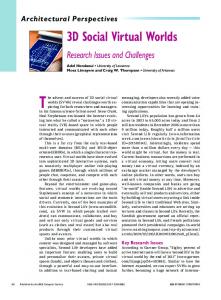
1.1 Enhancing the perception of user actions in 3D collaborative virtual environments A Collaborative Virtual Environment (CVE) is used for collaboration and interaction of participants that may be spread over large distances. The applications are usually based on networked virtual environments where the users interact through avatars. An avatar is a representation of a person in the virtual environment. Avatars can communicate with each other as well as doing activities that people do in their daily life. Nowadays, virtual environments like Second Life (SL) attract many people to experience 3D virtual life. In Second Life, residents can explore, meet other residents, socialize, participate in individual and group activities, and create and trade virtual property and services with one another, or travel throughout the world. Virtual environments can be also used to increase interaction and immersion in e-learning systems (Li, et al., 2009) or teleconferencing (Figure 1-1). People can attend virtual meeting rooms (teleconferencing) or virtual classrooms (e-learning). They can discuss with other people (avatars) and interact through virtual resources (e.g. blackboards, shared tables, etc.).

Figure 1-1: Avatars meeting and interacting in a 3D virtual space (OpenSpace3D, 2010) Avatars are animated by their human counterpart to provide a sense of telepresence. The animation of avatars allows users to express themselves in the virtual environment and helps to focus attention on objects of interest (Horain, et al., 2005). However controlling their behaviors is difficult. Selecting animation primitives from a menu or using icons is tedious. Moreover the avatar animation is not lively as it moves only on command. There are a number of efforts underway to make 3D animated human form more lifelike and to achieve more intuitive interaction (e.g. Avatar Puppeteering by Linden Lab (Linden, 2010), Hands Free 3D by Kapor Enterprises (Kapor, 2010)). We propose to enhance the perception and immersion of users in 3D virtual environments through 3D motion capture by monocular vision. In this way, the avatar can mimic the gestures of the user in real-time. This increases the users‟ sense of presence in the 3D virtual space (Marques Soares, et al., 2004). In this type of immersion, users do not have to memorize a large number of commands to use any special capture device. Motion capture by 22

monoscopic computer vision offers a flexible solution as only a single camera is required, thus allowing telepresence to anyone using a personal computer with a webcam. In this work, monocular vision (from a webcam) is used since webcams are very low-cost and flexible consumer devices (commonly included in personal computers and netbooks), in contrast to recent consumer devices capable of providing 3D information (e.g. camera TOF, Kinect), which are generally more costly and less flexible. We aim to allow the users to fully control and express themselves via their 3D avatars (Figure 1-2). 3D human motion is captured through a webcam using computer vision algorithms and rendered by his avatar in real-time. This kind of immersion allows new gesture-based communication channels to be opened in virtual inhabited 3D space (Horain, et al., 2005).

Figure 1-2: Our target application: 3D motion capture for 3D collaborative virtual environments (MyBlog3D, 2010).

1.2 Other potential applications Motion capture technology has a wide variety of highly demanding applications. At present, the film industry is the application where motion capture is most extensively used. Motion capture techniques allow large amounts of animation data to be produced; the movements of human subjects (athletes, dancers, actors) are captured and transferred directly or indirectly to computer-generated animation models. This gives animator the ability to produce more realistic movements. Movies use mocap to replace traditional animation by hand and also to produce computer-generated creatures that interact visually with real actors (e.g. the Gollum character from the Lord of the Rings film). Recently, several films and television series have been produced almost entirely using motion capture animation (e.g. The Polar Express, Avatar, etc.). Similar motion capture techniques are applied in videogame industry to allow more convincing and realistic character movements and expressions. Gait analysis is the systematic study of the body‟s motions in space (kinematics) and the forces producing them (kinetics). In clinical medicine, gait analysis is applied to humans in order to identify pathological disabilities (e.g. neuromuscular disorders, cerebral palsy). Since early 1970s, this analysis was done by careful frame by frame study of the videos provided by 23

a camera system. More recently, motion capture technology has been applied to gait analysis in order to quantify the movements (Cloete, et al., 2008), (Saboune, et al., 2005). This allows the joint angles to be compute more accurately and the contribution of each bone and muscle to be detected in the motion trajectory. Variations in gait style (walking speed, step length, cycle time) can be also used in biometric identification and in sports performance enhancement. Recently, some entertainment applications have started using motion capture in order to provide more intuitive forms of interaction in human-machine or human-software interfaces. In the videogames industry, the next step is to allow players to interact with games using only body motion or gestures (hands-free gaming) without holding any physical device (e.g. Kinect from Microsoft, EyeToy from Sony). Human-robot interaction is another example of a motion capture application. A major challenge in robotics is providing humanoid robots with embedded intelligence so they can autonomously interact with people by using natural nonverbal communication (human gestures). Embedding motion capture in a robotic system would provide two advantages: 1) understanding meaningful human gestures and movements in order to serve humans in their daily life (Kanda, et al., 2003), 2) communicating effectively with humans by imitating as closely as possible their natural motions (Kim, et al., 2009), (Nakaoka, et al., 2003). This would allow robots to participate in many human society activities. Automated video surveillance is another demanding application for human motion capture. Video surveillance can be used in geriatric-care, alarm security systems, home-nursing, etc. The goal of automated surveillance is to reduce the large number of human operators required to monitor many real time video feeds simultaneously by using software that can analyze video content automatically. Currently, automated video surveillance is an active research area in computer vision with many remaining technical challenges (Dick, et al., 2003). In order to develop automated surveillance system, motion capture could be used to detect, track, identify people, and generally, to analyze human behavior in real-time without the need to attach any joint markers. These systems must be able to operate in public spaces (unconstrained environments) where lighting variations, occlusions and changes reflectance represent a significant challenge for the computer vision analysis.

1.3 Main challenges We focus on 3D motion capture by monocular vision in real-time without markers (Horain, et al., 2002). This computer vision problem is inherently difficult because of insufficient information from images, ambiguities in the projection of monocular images, the large number of human pose parameters to estimate and self-occlusion of body parts. In this section, we describe the main challenges addressed in this work. Lack of depth information: inferring the 3D pose from images obtained with only one camera is an ill-posed problem. Forward and backward movements with respect to the camera‟s viewpoint (depth direction) lead to more than one possible solution due to the ambiguities in monocular images. These ambiguities result in motion-mistracking. High-dimensional search: in order to estimate the 3D human pose, several works (Sminchisescu, et al., 2002), (Delamarre, et al., 2001) use a 3D human model to infer the correct joint angle values (degrees of freedom) of each body part (head, neck, arms, forearms, 24

hands, legs, etc.). Some other works (Ramanan, et al., 2003), (Noriega, et al., 2007) try to infer the position of each body part separately before enforcing joint connectivity. In both cases, the number of parameters to be estimated is very high (between 20 and 60 dimensions); therefore, finding the optimal pose is a search problem in a high dimensional space. This requires intensive computation that is difficult to achieve real-time. Occlusions of human body parts: tracking 3D human motion from monocular images can become a difficult task as there are poses where some body parts are occluded by others (e.g. walking, arms crossed). In order to cope with occlusions, several works (Ning, et al., 2004), (Sidenbladh, et al., 2002) use a learned motion model or exploit a temporal coherence in order to track the pose through body parts occlusions. Clothing variations: different clothing in humans can be a problem (e.g. clothing of different shapes, or with color, edges and complex textures) causing inaccurate observations leading to ambiguities and consequently, incorrect 3D pose estimates. Variations in human body proportions: many 3D pose estimation techniques (Deutscher, et al., 2000), (Sminchisescu, et al., 2002) use a 3D computer model of the human that must be matched to the actor in the image. Such model usually has predefined body part sizes and shapes. Thus, if the human model has different proportions from the real subject, the matching between the model projections and the actor cannot be accurate and failures may occur. For example, if the arms of the model are larger than the arms of the subject, the model arms can intersect erroneously with other body parts. General motions: several works on 3D motion capture (Urtasun, et al., 2004) use learned motion models to track cyclic or repetitive motions (e.g. walking, running, golf swing) however, general motions are difficult to track as they are highly variable and unpredictable, making the learned model useless. Several works address the problem of tracking general motions by propagating multiple hypotheses at each time (e.g. particle filter approaches), this often provides robust and accurate results, however, computation times can be very high as a large number of hypotheses must be propagated. Complex environments: lighting changes and cluttered or dynamic backgrounds (e.g. public spaces) from video sequences can be a problem as imprecise observations (e.g. clutter edges, segmentation failures) can make the pose estimation procedure fails. Lighting changes can cause misclassifications in color segmentation or the emergence of new segments in the scene. Shadows, textures and objects in cluttered backgrounds can produce distracting image measurements (e.g. color, edges, optical flow).

1.4 Thesis contributions In this thesis, we extend the approach proposed in (Marques Soares, et al., 2004) and we propose new methods to achieve real-time 3D motion capture by monocular vision. The work is organized as follows. Chapter 2 is a detailed analysis of the state-of-the-art for 3D motion capture by computer vision. Recent works in this area are discussed, emphasizing their respective benefits and limitations. Finally, we describe our baseline approach for real-time 3D motion capture by monocular vision. 25

In chapter 3, new algorithms are proposed to enhance the tracking performance of our baseline approach. We describe a new method that combines a robust region-based registration step and a more accurate edge-based registration step. The respective limitations and benefits of these are compared experimentally. Finally, we derive an optimal trade-off curve between these steps that achieves the best accuracy possible given the real-time constraint. In chapter 4, we address the limitations of local optimization algorithms for 3D motion capture by introducing an improved set of optimization heuristics for real-time particle filtering. We describe and experimentally evaluate a number of heuristics that we demonstrate to jointly improve both the robustness and the accuracy of real-time 3D motion capture by monocular vision. End- effector based pose parameterization is introduced to handle the intrinsic data uncertainties more robustly. Real-time computation with large number of particles is achieved using a parallel GPU-based implementation of the particle evaluation step. Finally, we experimentally compare the results of our proposed real-time particle filtering algorithm on several real video sequences. In chapter 5, we summarize the contributions of the thesis and present our final conclusions. Perspectives and further extensions are also discussed.

26

Chapter 2 State of the art 2.1 Introduction The use of motion capture technology is relatively new; it began in the late 1970‟s for military purposes (tracking movements of pilots) (Maureen, 2000). Later, in 1980, Vicon Motion Systems created the first system for gait analysis, which the captured motion of children in order to detect disabilities (Sutherland, et al., 1988). Since the 1990‟s, advances in computer processing power and research in algorithms have made possible a wide variety of new applications (see section 1.2) including real-time motion capture computation (Molet, et al., 1996). Nowadays, motion capture is rapidly becoming cheaper and many more systems have emerged in the market. However, it still faces challenges, such as lack of precision of the motion data and complicated calibration procedures (e.g. special environments, uncomfortable user equipment). In the following sections, current technologies for motion capture are described (section 2.2). Section 2.3 summarizes existing techniques for motion capture by computer vision without markers. Finally, section 2.4 briefly describes our baseline approach for 3D motion capture by monocular vision.

2.2 Motion capture technologies Mocap technologies generally include synchronized cameras and special suits with markers or sensors worn by the performers. Markers are set at body parts (or joints) and are tracked in order to identify the motion by their positions or angles. Only the motion of the actors, not their visual appearance, is recorded and this motion is the mapped to a 3D model by computer. Motion capture techniques can be classified by their input methods, namely optical, mechanical, magnetic, acoustic and inertial. Each of these inputs (or a combination of them) is tracked, ideally at least twice the frequency of the desired motion.

2.2.1 Optical systems In optical motion capture systems, data acquisition is implemented using special markers attached to the actor (Optitrack, 2010); this approach uses at least three synchronized cameras and proper lighting to estimate the performer's position in 3D space. These systems produce data with 3D locations for each marker (Figure 2-1). Two types of markers can be used: passive and active.

27

Passive markers: Passive optical system use markers coated with a retro-reflective material to reflect back light that is generated near the cameras lens. The operating principle is similar to radar: the cameras emit radiation (usually infrared), which is reflected by the markers and returned to the same camera. The cameras are sensitive to a narrow band of wavelengths and perceive the markers as bright spots. Such a system typically consists of 6 to 24 cameras. Passive systems do not require the user to wear wires or electronic equipment. The markers are usually attached directly to the skin, or to a full body lycra suit designed for motion capture (Qualisys, 2010). Active markers: Rather than reflecting back externally generated light, the markers themselves are powered to emit their own infrared light. Active optical systems triangulate positions by illuminating one LED at a time very quickly or multiple LEDs with software to identify them by their relative positions. Some systems can modulate the amplitude or pulse width in order to provide marker ID. This unique marker ID provides much cleaner data than passive marker systems (PhaseSpace, 2010).

Figure 2-1: Optical motion capture system. Actor wearing an optical motion capture suit with infrared markers (left). 3D human pose inferred from the relative positions of each marker (right) (PhaseSpace, 2010).

2.2.2 Mechanical systems Mechanical methods use an exoskeleton – a skeletal-mechanical structure attached to the performer‟s body (Figure 2-2). The exoskeletons are rigid structures of metal or plastic rods that articulate at the joints of the body linked together with potentiometers. They directly track body joint angles by the sensors attached to the exoskeleton. They provide real occlusion free information, however, the exoskeleton suit can be heavy and cumbersome, limiting the user‟s freedom of movement (Gypsy7, 2010).

28

Figure 2-2: A mechanical exoskeleton suit for motion capture (Gypsy7, 2010).

2.2.3 Magnetic systems Magnetic systems use sensors placed on the body to measure a low-frequency magnetic field generated by a transmitter source (Figure 2-3). The outputs of these sensors are 3D positions and rotational information. The number of sensors used is usually from 6 to 11. The sensors and source are attached to an electronic control unit that correlates their reported locations within the magnetic field (AMM, 2010). Inverse kinematics (IK) is then used to recover the angles for the different body joints. A big advantage of these systems is that useful real-time results can be obtained from only 6 sensors. However, the sensors are susceptible to magnetic and electrical interference from metal objects in the environment. In addition, the wiring from the sensors tends to limit the actor‟s movements. Recently, the development of new wireless magnetic systems has been reported (Kanetaka, et al., 2010).

Figure 2-3 : A performer wearing a suit for magnetic motion capture (AMM, 2010)

2.2.4 Acoustic systems Acoustic systems use three audio receivers and an array of audio transmitters on the performer‟s body. The audio transmitters send clicking sounds and the receiver measures the travel times from each transmitter (Intersense, 2010). The calculated distance from the three receivers is triangulated to provide a point in 3D space. This position data is typically fed to an inverse kinematics system which in turn drives an animated skeleton. An advantage of this method is the relative absence of occlusions. Unfortunately, accuracy may be affected by sound reflections or audio interference.

29

2.2.5 Inertial systems Inertial systems are based on miniature inertial sensors (gyroscopes and accelerometers) with sensor fusion algorithms to measure the rotational rates. Motion data is transmitted wirelessly to a virtual skeleton in software. Basically, these systems are similar to the Nintendo Wii controllers but are more sensitive and more accurate. Inertial systems are practical because they are portable and do not require large capture areas or complicated calibration (IGS-190-M, 2010). A disadvantage is that the positional drift that can compound in time if the setup is not correct due to poor calibration.

2.2.6 Computer vision based systems Using computer vision techniques to acquires the human body motion is one of the most attractive and practical solutions as it does not require any expensive or invasive hardware or markers (only cameras are required) and it can work outdoors (in streets, offices, parks). Algorithms have been proposed that capture human motion at near real-time frame rates; however, they mostly rely on multi camera systems under controlled conditions, which limit their applicability. Some monocular vision approaches (Agarwal, et al., 2006), (Urtasun, et al., 2006) aim at capturing specific motions (walking, golf swinging, jumping, etc.) using some learning model or tracking motion for certain parts of the body. Some other systems can track unconstrained motion, but do not run in real-time (Sminchisescu, et al., 2003). Recently, 3D image sensors have been used to capture the 3D body shape and disambiguate poses using depth measurements. Time-of-flight sensors (Ganapathi, et al., 2010), (Kolb, et al., 2010) and active triangulation system (e.g. Microsoft Kinect (Kinect, 2010)) are such dedicated sensors. Real-time markerless tracking of human pose by monocular computer vision remains a hard yet relevant problem.

2.3 Human motion capture by computer vision Human pose estimation from images is an unsolved and currently active field of research with significant scientific and computational challenge (Sminchisescu, 2007). As this is the main topic of this work, we present a more detailed analysis of computer vision-based techniques. We consider both real-time and non-real-time systems, as well as single and multi-camera systems. Systems for motion capture using computer vision are first discussed based on the image descriptor or features that they use (section 2.3.1). Human pose can then be estimated using a generative approach (section 2.3.2) or a discriminative approach (section 2.3.3) (Sminchisescu, 2007). Tracking the pose between consecutive frames of a video sequence can ensure the temporal coherence of the human motion (section 2.3.4). Finally learned motion models can be used to enhance the robustness of the motion tracking (section 2.3.5).

30

2.3.1 Image features for motion capture In order to estimate the 3D pose, image features are extracted from input images. A feature or image descriptor can be defined as a piece of low-level visual information extracted from an image to solve a specified task. Image descriptors are generally extracted using probability distributions (e.g. color histograms), neighborhood operations (e.g. edges, optical flow) or thresholding the pixel values (e.g. foreground or color classification). The choice of features depends greatly on the problem to be solved. In human motion capture, the image descriptors are generally used as cues to find the position of each body part and thus to estimate the full 3D human pose. Image descriptors commonly used in the literature include color, silhouettes, edges and motion (Poppe, 2007), (Moeslund, et al.).

2.3.1.1 Color Skin color is a common cue for head and hand detection (Vezhnevets, et al., 2003). Broekhuijsen et al. (2006) extract skin regions by converting images to the HSV color space, thresholding each channel empirically, and finally selecting the largest connected components, which are deemed to belong to the head and the hands. Bernier et al. (2009) use an initial face detection algorithm to obtain a normalized skin color histogram in the UV chrominance space (from YUV color space). A skin color probability is estimated from the histogram and then used to detect the head and hands. Some human motion capture works combine different color cues into a single probability; Fontmarty et al. (2007) define a color-based likelihood that combines clothing color and skin color. For clothing probability, a learned reference histogram of the clothing color is compared using a Bhattacharyya distance with a targeted ROI in the image. In addition, they calculate a homogenous distance by measuring the standard deviation of the color distribution in RGB space from uniformly sampled points inside the color region. Unfortunately, color may lack robustness in cases where significant local changes in illumination can occur. In addition, cluttered scenes that contain colors similar to regions of interest (skin or clothing) can generate noise in color segmentation.

2.3.1.2 Silhouettes When capturing images with a static camera, silhouettes can be obtained using background subtraction techniques (Figure 2-4). Silhouettes can encode useful information about the human pose. Shahrokni et al. (2004) extract the human silhouette by texture segmentation. Deutscher et al. (2005) extract the silhouette by a thresholded background subtraction algorithm. Agarwal et al. (2006) encode the shape information of learned silhouettes by computing histograms of shape context descriptors (Belongie, et al., 2002) that can be compared using simple Euclidean distance. Silhouettes output by background subtraction can be noisy due to illumination changes or shadows, which can affect their shape. Another limitation is the poor visibility of certain degrees of freedom (e.g. knees, elbow, hands), which causes a high degree of ambiguity and body part occlusions which make it difficult to recover the 3D human pose.

31

Figure 2-4 : Human silhouettes extracted using a background subtraction algorithm (Howe, 2006).

2.3.1.3 Edges In computer vision, an edge is a significant variation or discontinuity in the gray level of a digital image. Edges detector algorithms provide the set of connected curves that indicate the boundaries of objects of interest (Ziou, et al., 1998). In human motion capture image edges are a useful cue for the boundaries of body limbs (e.g. hand, arm, head, forearm, etc.). Some works (Fontmarty, et al., 2007), (Chen, et al., 2005) compute a distance transform to measure the distance between edge points in the image and their nearest pixel on a candidate silhouette boundary. Other works (Ramanan, et al., 2003) use edgeS as a cue to detect or track body parts (e.g. arms, forearms, hands). Broekhuijsen et al. (2006) estimate the hand position by computing the number of edge pixels along a skin region of the full arm. They also train edge response histograms of limb-like edges and background-edges. They compute the probability that an edge belongs to a body part according to the edge orientation. Noriega et al. (2007) use the orientation of the edges to estimate the position and orientation of a limb. Edges have the advantage that they are very robust to changes in lighting conditions and can be extracted at a very low computational cost. However, undesirable edges resulting from background clutter, clothing textures edges or noise may be a problem. 2.3.1.4 Motion Motion capture may use optical flow (Horn, et al., 1981), (Lucas, et al., 1981) to directly estimate the motion of each human body part by assuming small motion and brightness constancy. Ju et al. (1996) use a parameterized optical flow equation to recover the motion of each region belonging to the limb. Bregler et al. (2004) write the analytical relationship between the vectors of apparent motion in the image and the angular change of each joint. In this technique, linear differential equations need to be solved in order to update the 3D pose parameters for each frame. Sminchisescu et al. (2001) use an optical flow method that generates a flow field with an outlier map that provides information about the motion boundaries. Noriega et al. (2007) detect motion by computing the difference between the pixels of consecutive frames. They calculate a motion energy score for each limb. Motion cues are usually robust to extract and provide useful information about the direction of the movement of each body part; however one disadvantage is the assumption that the 32

person is always moving in the scene. Moreover, optical flow assumes small motions between frames; this is not always the case for human motion (especially motions of the arms and legs). Additionally, the deformation of clothing as a person moves can make the motion estimation difficult. 2.3.1.5 Feature combinations Some works integrate different cues to achieve more robustness in the 3D pose estimation. Several methods have been used to combine the information from different descriptors. Chen et al. (Chen, et al., 2005) combine the silhouette information with edges extracted from the same silhouette. They extract edges from the foreground silhouette and compute a distance transform to the silhouette boundaries. Sminchisescu et al. (2001) combine edge and motion information in a negative log-likelihood function. Edges are weighted according to their importance qualified by a motion boundary map extracted from an optical flow method. Fontmarty et al. (2007) combine edge distance, color, and 3D blob distance (acquired from two cameras) into a single observation function. They assume that all observations are mutually independent probabilities. Combining image descriptors proves to be more robust as the advantages of each descriptor can be used in one or more likelihood functions. However, care must be taken because each descriptor can give incompatible likelihoods.

2.3.2 Generative approaches These approaches estimate the human pose using a prior model of the human body, parameterized by the kinematic tree of the articulations and the body dimensions. The pose of the human body model is described by a vector of parameters. Generative approaches differ essentially in the manner in which data is associated with the 3D model. In this case, we can identify two methods: reconstruction-based and appearance-based. The first method (reconstruction-based) try to fit the 3D model to a 3D cloud obtained from multiple cameras (Urtasun, et al., 2004), (Ziegler, et al.). In the appearance-based techniques, a human model with a defined pose is projected into the input image and several features (section 2.3.1) are extracted from the image (Lee, et al., 2002), (Ramanan, et al.), (Sminchisescu, et al., 2003). In both techniques, the human pose is estimated by finding the vector of model parameters that best fits the input data. Finding the pose that best matches the image features can be a very difficult task, because occlusions of body parts may occur and same image feature can match different 3D poses (ambiguities). Several works propose different human body models and methods to estimate and track the human pose over time. Some learning methods are also used to improve the motion capture results. These methods will be described below. 2.3.2.1 Human body models Human models are basically represented with a kinematic tree that of rigid segments connected by articulated joints. Each segment represents a specific human body part and can be described by a 2D figure or a 3D volume. A joint may hold up to 3 degrees of freedom. A given pose of the model is described by a vector of parameters of joint angles.

33

Morris et al. (1998) proposed a simple 2D scaled prismatic model (SPM). In this model, each segment is represented as a line that contains two parameters: the angle rotation and its length. Each segment contains a translational degree of freedom that scales the link appearance in order to estimate 3D motions. This model does not require specification of link lengths and joint axes. The author argues that such 2D SPM‟s avoid some of the singularity problems associated with 3D motion from monocular vision. Cham et al. (Cham, et al., 1999) used the SPM‟s in order to estimate 2D human motions from monocular sequences. A simpler 2D model is used by Mamania et al. (2004), this model is represented by a stick figure (Figure 2-5), where the articulations are represented as points and the body parts or segments as simple lines.

Figure 2-5 : A human body model represented by a stick figure (Mamania, et al., 2004). Ju et al. (1996) represent the human model as a set of connected 2D planar patches (Figure 2-6). A kinematic tree is constructed from these patches. Each patch is represented by its four corners, which represent also the articulation points between two connected planar patches. A similar model is used by Para et al. (2008), where each body part consists of 2D planar figures (circles and rectangles) that are linked with flexible joints. Each planar figure contains three degrees of freedom which include the 2D coordinates of its centre and the rotation angle around the axis perpendicular to the image plane.

Figure 2-6 : A human body model represented by 2D planar patches (Ju, et al., 1996). 34

Because 2D models are not able to capture the 3D motion correctly, many works add 3D volumes around the segments of the kinematic tree to represent more accurately the 3D pose (Figure 2-7). Deutscher et al. (2005) use a full body model that consists of 17 segments and 29 degrees of freedom. Each segment is fleshed out by cones with elliptical cross-section. The author argues that such models have many advantages including computational simplicity and compact representation. Several works have adopted similar models. Saboune et al. (2007) use a model formed by 19 joints that represent key elements of the human body (head, elbows, knees, arms, etc.), each segment is fleshed out by adding cube volumes around it. Azad et al. (2004) use a model with 28 degrees of freedom, where each body part is modeled as a section of a cone. Each cone is described by two ellipses (base ellipse and upper ellipse) and the length between these ellipses. Noriega et al. (2007) combine 2D patches and 3D volumes to represent an upper body model. Arms and forearms are modeled as cylinders and the head as a sphere. The torso, hands and clavicles are represented by 2D planar patches. Limb interactions are described in terms of distances between the body parts.

Figure 2-7 : A human body model represented by 3D volumes (Azad, et al., 2004)

To achieve a better approximation of the human shape, some 3D models are constructed by polygon meshes. Sminchisescu et al. (2001) use a mesh model that consists in a kinematic structure covered by super quadrics ellipsoids (Figure 2-8). This model is described by 30 joint parameters, 8 internal proportion parameters encoding the position of the joints and 9 deformable shape parameters for each body part. The shape parameters are based on standard humanoid dimensions.

35

Figure 2-8: A human model represented by super quadric ellipsoids (Sminchisescu, et al., 2001)

2.3.2.2 Pose estimation Pose estimation refers to the process of searching for the set of model parameters that minimizes the similarity between features extracted from the model and the input image using local optimization. The model parameters can be the joint angles or the global positions of each body part. Due to the high-dimensionality of the model parameters (20 or more joint angles), the search method used must be very efficient. In the state of the art, many works take several minutes per frame and only few can achieve quasi-real-time results (Hua, et al., 2007), (Fontmarty, et al., 2008), (Bernier, et al., 2009) In general, there are two techniques for generative pose estimates: top-down estimation and bottom-up estimation. Related work using these approaches will be described below. 2.3.2.2.1 Top-down estimation Top-down approaches estimate the state vector describing the human pose at each frame by a local search that evaluates different candidate poses starting from the configuration found in the previous frame (Figure 2-9). One drawback of this approach is the pose in the first frame must be specified manually by the user. In (Bregler, et al., 2004), the user must click on the 2D joint locations in all camera views at the first time step. The correspondence between the 3D pose and the image projection is found by minimizing the sum of squared differences between the projected model joint locations and the user supplied model joint locations. The optimization is done over the poses, angles, and body dimensions. The global minimization over all parameters yields a tri-linear equation system whose solution is approximated with a Quasi-Newton method.

36

Figure 2-9: Generative Top Down estimation: 1) Input image, 2) Image feature, 3) Model projected in a candidate pose, 4) Estimation of model parameters by matching model projection and input image features (Sminchisescu, et al., 2002).

Finding the best match can be computationally expensive due to the high number of parameters (dimensions) to be estimated. Different search strategies have been proposed; Delamarre and Faugeras (2001) created forces from the extracted human silhouette to the projected model. These forces are inferred from a comparison between tangents to the contours of the tracked object and the model. The forces are applied to the 3D model in order to push it towards the silhouette in the images by solving dynamical equations iteratively until convergence. Grest et al. (2007) used the normal displacement between the contour points of the model projection and the silhouette to estimate a Jacobian Matrix, which allows analytical derivation of the optimization function. Although the use of analytic Jacobian allows the number of iterations for pose estimation to be reduced, spurious local minima persist because observation likelihoods are typically multi-modal (Sminchisescu, et al., 2002). Instead of using non-linear optimization techniques, some authors try to simplify the problem by fitting the model directly to the observations. Niskanen et al. (2004) use an articulated surface like a human model. They use a set of 2D silhouettes (from multiple views) that are combined together with multi-camera geometric constraints. The human surface model is fitted to the 3D observations by the minimization of an objective function that takes into account the location and orientations of these observations. Taylor (2000) proposes a method to estimate the 3D pose directly from 2D points. In his work, the correspondence between joints in the model and point features in the image is provided by the user. The relative length of the segments in the model is also known a priori and the depth ordering of the image points must be specified manually. The 3D pose is then deduced from foreshortening of the body segments of the model under a scaled orthographic projection. Thus, they directly recover the coordinates of the joints in the world coordinate system. 2.3.2.2.2 Bottom-up estimation Bottom–up approaches detect each body part individually from image features and assemble the detected parts together into a human body pose using heuristics or constraints such as the proximity between linked body parts. These approaches have the advantage that they can automatically perform initialization and recover from tracking failures. Furthermore, highdimensional search is avoided by partitioning the joint pose space into separate sub spaces for 37

each body part. However, the main difficulty is that body parts are not easy to detect producing many false positives as there may be many limb-like regions in an image. Various authors have proposed techniques to track body parts using image features and to infer the resulting full body configuration. Ramanan and Forsyth (Ramanan, et al., 2003) proposed body part detectors based on appearance and parallel lines. They learn the appearance of body parts by modelling segments as cylinders. Then, they convolve each frame with a template that responds to parallel lines of contrast. A feature vector (a normalized histogram in Lab space) captures its appearance of each candidate segment. They cluster the body part appearances and connect up the kinematically valid clusters with a dynamic Bayesian net. Hua et al. (2007) use detected edges of the contour of each limb. Each individual limb is represented by its own motion parameters. An undirected graph represents the spatial coherence among different body parts. They reinforce the spatial coherence constraints between neighboring parts using a Markov network. Several works use multiple cues to enhance the robustness of body part detection. Noriega et al. (2007) use color information, contours, background subtraction and motion to detect upper-body parts. The head and hands are identified using color information; the torso is detected using a rectangular grid of points interacting with a foreground silhouette; the arms, forearms and shoulders are detected robustly by fusing contour based cue and motion energy. Upper-body parts are represented by spheres, cylinders and 2D patches. The upper body is modeled as a factor graph with limbs represented by nodes and links corresponding to articulations and non collision constraints between limbs. The complete graph includes the previous states to take temporal coherence into account. Broekhuijsen et al. (2006) use specialized detectors for the different joint and end-effector locations. Each detector uses a set of image descriptors. Background subtraction is used to identify the regions of the human silhouette. A template containing an outline of the head and shoulder is fitted to the extracted silhouette in order to obtain the 2D locations of the shoulder, neck and head. Skin color features are used to find the regions that belong to the head and arms. Edge response distributions (histograms) of limb-like edges and background-edges are compared to find the width of the lower and upper arm in the images. The 2D locations of the elbows are estimated by intersecting the lines through the centers of the lower and upper arms. Although body part detectors based in multi-visual cues have proven to be more robust, unobserved body parts caused by self-occlusion may still give rise to motion mistracking. 2.3.2.2.3 Combining Top-down and Bottom-up estimation Some authors combine Top-down and Bottom-up approaches to address the limitations of each. In other words, they use the detection of body parts to improve the robustness in the estimation of the human pose parameters (e.g. joint angles). Lee et al. (2002) fit a body model projection to a human silhouette and identify the position of hands, head and torso from the silhouette boundaries. The hands are detected along the outlines of the silhouette by extracting peaks in the convex curvature. The head is detected using a reference template representation of a head-shoulder contour. The torso is found by extracting the medial axis from the 2D silhouette. They then infer the human pose analytically by estimating the joint angles using geometry and inverse kinematics. Fontmarty et al. (2008) estimate the 3D pose by matching the human model projection with the foreground silhouette. In addition, they use skin color segmentation from two cameras to obtain 3D blobs that belong to the head and hands regions. 3D pose configurations are computed using 3D hand 38

and head positions by an analytical Inverse-Kinematics (IK) algorithm. Analytical 3D pose configurations are used to initialize automatically, recover from tracking failures, and guide search in the high-dimensional state space. Sminchisescu et al. (2006) propose an algorithm for learning a bidirectional function model that combines Top-down and Bottom-up processing for monocular 3D human motion estimation. Both learning process are done in alternative steps of self-training that optimize the probability of the image evidence: the Bottom-up process is tuned using samples from the Top-down process and the Top-down process is optimized to produce inferences close to the ones predicted by the current Bottomup process. Both processes converge at equilibrium, generating a consistent bi-directional function. The framework provides a uniform treatment of human detection, 3D initialization and 3D recovery from tracking failures.

2.3.3 Discriminative approaches Discriminative approaches do not use an explicit human body model based representation. Instead, they infer the human pose directly from the image observations or features, using training examples to establish a direct relationship (or mapping) between the image observations and human poses; this assumes that the set of typical human poses is far smaller than the set of kinematically possible ones. Therefore, the training data needs to generalize well to observed variations over body configuration, body dimensions, viewpoint and appearance. The mapping method must also account for the highly non-linearity of the mapping between the feature and the pose space These approaches have the advantage of avoiding the need for explicit initialization and accurate 3D modeling and rendering. They can also be used to initialize generative approaches as in (Fossati, et al., 2007). However, they require a sufficient number of training examples in order to infer human pose properly, and they tend to be more sensitive to background clutter than generative approaches because an explicit model is not available for background masking. Pose estimation techniques using discriminative approaches can be divided into two classes: learning-based estimation and example-based estimation. Related work using these methods will be described below.

2.3.3.1 Learning-based estimation In Learning-based estimation, a function that maps from image space to pose space is learned using training data (Figure 2-10). Learning a function that directly recovers pose estimates from low-level image features can be highly complex as the same image features can represent different body pose configurations and same body configurations can generate different image features due to ambiguity. One of the first contributions was proposed by Rosales et al. (2000), who clustered (with Expectation Maximation algorithm) the space of 2D body poses into approximately homogeneous configurations. Then, for each cluster, a function was estimated to build the mapping from human silhouettes to 2D pose. This mapping was modeled using a neural network. For each new image, the mapping of each cluster is performed to yield a set of possible poses or solutions. From this set, they select the most likely pose by finding the best match using the maximum likelihood criterion. Grauman et al. (2003) used PCA to build a probability density of multi-view silhouette contours augmented with 3D structure parameters (the 3D locations of key points on each silhouette). In this way, the mixture model represents a density for the image contours together with their 39

associated 3D structure parameters. Then for a given multi-view input contour, they essentially treat the unknown 3D structure parameters as missing variables, and find the MAP estimate of the shape and structure parameters based on the input contour data. They resolved the ambiguities of image silhouettes using the multi-view contours from cameras at known locations. Elgammal et al. (2004) learned an explicit low-dimensional nonlinear representation of an activity manifold from visual inputs (human silhouettes). They also learned mapping functions between such representations and both the visual input space and the 3D body pose space. In order to recover the human body pose, they projected the visual input (silhouette) to the learned low-dimensional manifold and then found the point on these manifold corresponding to the visual input using an embedding space error metric. A similar idea was adopted by Guo et al. (2007), who applied Gaussian Process Dynamical Models (GPDM) (Urtasun, et al., 2006) to obtain two low dimensional nonlinear manifolds: one corresponding to the local joint angles and the other manifold the space of silhouettes for different views. Then the nonlinear mapping between these two low dimensional spaces is learned using a Sparse Relevance Vector Machine (RVM). Agarwal and Triggs (2006), (2004) encoded the shape of the human silhouette using histograms of shape contexts, which provides a significant amount of pose information. They applied Relevance Vector Machine (RVM) to model the nonlinear relationship between the histograms of shape contexts and the 3D poses. In order to reconstruct 3D human pose from ambiguities in monocular images, they used a mixture of regressors scheme that give multiple possible poses (Figure 2-10). Sminchisescu et al. (2005) also used shape context to encode the appearance of human silhouettes. Their training data consisted of pairs of typical human configurations together with their realistically rendered 2D silhouettes. They learned the multi-valued nature of the mapping from observations to pose states with a Bayesian Mixture of expert model. Each expert transforms their inputs into an output prediction and these are combined in a probabilistic mixture model based on Gaussians centered on them. The result is a conditional mixture distribution with components and mixing probabilities that are inputdependent. In this way, the inference of 3D pose is straightforward as the most probable mode can be selected. The authors showed promising results comparing their Bayesian mixture of experts (BME) conditional models with other methods like weighted nearest neighbor (NN) or the relevance vector machine (RVM). BME presented smaller average pose estimations errors.

40

Figure 2-10: 3D human pose reconstructed directly from silhouettes using learned RVM model (Agarwal, et al., 2004).

2.3.3.2 Example-based estimation Example-based estimation avoids an off-line learning process by storing a database of training examples whose 3D poses are known. Pose estimation is done by searching for training images similar to a given input image, and interpolating from their 3D poses. One drawback of these approaches is the large amount of space needed to store the database, as exemplars sets can grow exponentially with object complexity. Example-based estimation approaches have proposed different methods to overcome this problem. Sullivan and Carlsson (2002) stored a set of key frames representing a specific action (e.g. playing tennis). In each of these key frames the body locations are determined manually. Then for every input frame of a video sequence, they use a shape matching algorithm based on qualitative similarity that computes point to point correspondence between shapes. Thus if any frame in the actual sequence matches to at least one key frame, the corresponding body locations are transferred from the matched key frames to the input frame using a closed loop tracking algorithm incorporating prior constraints (color and space constraints). The author argues that the use of key frames allows error recovery at any instant. Mori et al. (2002) adopted a similar idea; their approach consisted of storing a number of exemplar 2D views of the human body in a variety of different configurations and viewpoints with respect to the camera. On each of these stored views, the locations of the body joints (left elbow, right knee etc) were manually marked and labeled. The input image was then matched to each stored view, using the technique of shape context matching in conjunction with a kinematic chainbased deformation model. The locations of the body joints were transferred from the exemplar view to the input shape. These key points were used to construct an estimate of the 3D body configuration in the test image using the method proposed in (Taylor, 2000). Example-based estimation can also be embedded in learned probabilistic models. Toyama et al. (2002) used training exemplars to represent probabilistic mixture distributions of object configurations. Exemples are based on contours from silhouettes. The authors proposed the Metric Mixtures (M2) approach that combines a metric space with a probabilistic framework. 41

They applied the approach to track walking people using the chamfer distance algorithm on binary edge images. Stenger et al. (2003) proposed a tree based representation in a Bayesian probabilistic framework. The leaves of the tree define a partition of the state space with piecewise constant density. The advantage of this representation is that regions with low probability mass can be rapidly discarded in a hierarchical search, thus a significant speed-up can be achieved. Shakhnarovich et al. (2003) indexed training examples by learning a set of hashing functions. They proposed Parameter-Sensitive Hashing (PSH) which finds approximate nearest neighbors in sublinear time. In their algorithm, the hashing functions are sensitive to the similarity in the parameter space. They learned a feature space based on multi-scale histograms of edge directions. The results of their pose estimation were compared with the KNearest Neighbor method (k-NN). Fossati et al. (2007) relied on detecting key postures in a walking cycle. They linked sparse detections into a complete trajectory using a Viterbi-style algorithm. These detections included not only an example location but also the orientation of the person. In this way, orientation was used with a dynamic programming algorithm which allows the selection of the poses that provide the most likely trajectories according to the probabilities.

2.3.4 Pose tracking Pose tracking is the process of following and estimating the human pose from frame to frame in a video sequence. Tracking the human pose has several advantages: a) the difficult task of searching the high-dimensional pose space is alleviated as pose differences between frames are usually small, b) temporal coherence is ensured when dealing with image projection ambiguities, c) the complexity of the pose estimation is reduced as an initial pose estimate is provided at each frame. Generally, there are two strategies for tracking the pose: those that maintain or predict only one hypothesis (pose configuration) at each frame (single hypothesis tracking) and, those that propagate several hypotheses (multiple hypothesis tracking) or solutions per frame. Both approaches are described below.

2.3.4.1 Single hypothesis tracking A simple single hypothesis tracker simply updates the pose configuration changes over time. In (Bregler, et al., 2004), the pose and the joint angles are updated for each time frame using a local minimization criterion initialized from the pose in the previous frame. Ning et al. (2004) propose a tracking strategy that includes two stages: prediction and updating. In the prediction stage, the posture of the moving human in the current frame is roughly estimated from the motion in previous frames. Joint angles are predicted by calculating their rotational velocities in the previous frame and apply these to the kinematical equations. The subsequent stage, minimizes the matching error between the projection of the predicted posture and the edge image. Some authors use more complex techniques such as recursive linear filters (e.g. Kalman filter (Kalman, 1960)) to predict the human pose in each image. In (Rohr, 1994), the walking motion of pedestrians is tracked by assuming a linear relation between the model parameters and the measurement errors. The model parameters in the subsequent image are predicted by applying a linear Kalman filter (Kalman, 1960) with constant velocities for the model 42

parameters. Delamarre et al. (2001) predict the motion of each frame with a linear Kalman filter in order to accelerate the convergence of their pose estimation. They supposed that the time derivatives of the parameters of the 3D model are constant. In their experiments, more than half of the iterations were saved. However, the prediction failed in cases when the motion was large and the direction of variation of some parameters of the model suddenly changed, and also when occlusions of the 3D model lasted for too long. Unfortunately, single hypothesis tracking cannot deal with ambiguities, such as self-occlusion or image observations from monocular images. Therefore, there is always the possibility of selecting the wrong pose causing mistracking that may subsequent make recovery of the pose difficult. Deutscher et al. (1999) showed that using a Kalman filter to predict the motion of an articulated arm can lead to false results at kinematic singularities and at self-occlusions.

2.3.4.2 Multiple hypothesis tracking In order to overcome the problem of ambiguities in image observations, multiple hypotheses can be maintained and propagated from frame to frame. This can be done by adopting Sampling-based approaches such as Particle Filtering, e.g. the CONDENSATION algorithm (Gordon, et al., 1993), (Isard, et al., 1998). Particle Filters are sophisticated Monte Carlo methods that aim to estimate the sequence of hidden parameters (e.g. joint angles) based only on the observed data (e.g. image features). They approximate the posterior distribution by a weighted set of P particles or samples. Each particle represents a candidate human pose that can be compared to the extracted image features. Particle filter algorithms have the advantage that, with particles (and an accurate underlying model), they can cover the full posterior distribution in model space. Particle filters can also deal with nonlinear observation models, allowing the integration of multiple data sources into one observation model (data fusion) (Menezes, et al., 2011). However, when number of particles is not sufficiently large, the probability density function (pdf) of the human motion may not be represented sufficiently completely causing “particle depletion” and consequently, tracking failures. Furthermore, pose tracking the high-dimensionality of the pose space would requires the use of an impractically large number of particles for complete coverage. All the particles must be propagated and evaluated (weighted) according to a matching cost function. Therefore, large numbers of particles have a high computational cost. Recently, many works have proposed different schemes to guide the samples (particles) more effectively in the pose space and thus reduce the number of particles required. In one of the first such contributions, Deutscher et al. (2000) proposed to reduce the number of particles by using a multi-layered search to gradually migrate the particle set toward the global maximum, at the cost of multiple iterations of sampling per frame. Sminchisescu et al. (2001) proposed an efficient search technique that inflates each sample posterior covariance along uncertainty directions (covariance sampling) and refine each sample using continuous optimization. The image cost function is highly multi-modal in pose space, and guiding particles towards the wrong local minima may lead to mistracking. Some works use analytical inference to compute hypotheses from image observations or assumptions in order to guide particles directly towards “good” local minima. Sminchisescu et al. (2003) use simple kinematic principles to construct “kinematic interpretation trees” that contain the possible 3D body configurations associated with a given set of projected joint centres. The different 3D configurations are linked by „forwards/backwards flipping‟ moves, one for each kinematic 43

link. Lee et al. (2002) use analytical computation (inferred from the detection of body parts) to infer a subset of the state parameters, thus reducing the degree of dependence on the Monte Carlo simulation. They demonstrated a reduction in the required number of particles and the computational load. Fontmarty et al. (2008) computed 3D human pose configurations from possible 3D positions of THE head and hands using an analytical Inverse-Kinematics (IK) algorithm. Samples were produced using Quasi Monte Carlo sampling (Guo, et al., 2006) along the directions of lowest observability. Some modified particle filtering approaches introduce deterministic distribution sampling in order to search more efficiently in an optimal deterministic way. Saboune et al. (2005), (2007) propose a modification named Interval Particle Filtering that reorganizes the set of N particles into M subsets each formed of I particles covering in a deterministic way the “neighbourhood” of the j heaviest particles (j=1...M) of the previous frame. In this way, a larger number of neighbours I provide more accurate results but greater computational cost. Rose et al. (2008) introduce a particle filtering algorithm based on the Dynamic Bayesian Network (DBN) formalism that takes advantage of a factored representation of the state space to weight and select the particles. The factored representation is based on the dynamics of the joint angles. They used the factorization of the process to hierarchically resample the components of the state vector. Combining or fusing multiple cues or features can implicitly reduce the search space. Azad et al. (Azad, et al., 2007) fused edge cue from foreground segmentation and 3-D distance cues into one likelihood function. They used a standard particle filter approach to compare the properties of different cues. Fontmarty et al. (Fontmarty, et al., 2007) combined edge cues, color histograms, 3D blob distance and skin color into a global likelihood function assuming the mutual independence of each cue. Both authors proved to reduce the search space achieving quasi real-time results. However, multiple cues that are not well combined can drastically reduce the accuracy of the pose estimate. The number of particles can also be reduced by partitioning the high-dimensional pose space into several subspaces that belongs to each body part. Gang Hua et al. (2007) represent each individual limb with its own motion and enforce their spatial coherence with a Markov network. Motion posteriors of each body part are approximated by Bayesian inference and a set of low dimensional particle filters for each body part interact and collaborate with each other. Noriega et al. (2007) proposed independent particle filtering and likelihood evaluation for each limb, while taking into account interactions between limbs through belief propagation. They reported quasi real-time results (6 fps). Although these approaches provide reductions in the computational cost, self-occlusions may be a problem as unobserved body parts may give rise to motion mistrackings. Multiple hypotheses can also be maintained in time using a multi-dimensional non-linear optimization method. John et al. (2010) implemented a hierarchical particle swarm optimization (PSO) method to iteratively explore the high-dimensional poses pace using a population of multiple candidate solutions, named particles. The basic idea of PSO consists of simulating the unpredictable choreography of a bird flock in their search for food. The main difference between PSO and particle filter approaches is the fact that PSO uses particles to explore the search space while particle filters use particles to estimate the posterior density. In particle swarm optimization, each particle has its own velocity and communicates with other particles in order to perform the search. The authors combined hierarchical sampling with PSO in order to split the search space into 12 subspaces according to the kinematic human 44

tree. They presented comparative results with some particle filter approaches commonly used (Condensation (Isard, et al., 1998), Annealed particle filter (Deutscher, et al., 2000)), showing that the PSO paradigm outperforms particle filtering with small numbers of particles. They also noted that one of the main advantages of hierarchical PSO is the ability to initialize and recover efficiently from wrong pose estimates due to the effective communication between particles in the swarm search. However, the authors reported that hierarchical PSO paradigm only performs reasonably well using multiple cameras (4 to 8 cameras) while it fails in monocular video sequences, having problems with front-back ambiguities in which all body segments lie in the same plane.

2.3.5 Dynamic models Dynamic models can be used to encode the expected dynamics of a human motion, e.g. periodic motions such as walking, running, swinging, etc. They are used as predictive priors for tracking, providing more stable tracking at reduced computational cost. They are often learned from training data (e.g. body pose parameters) acquired with a motion capture system (section 2.2). Using such models, the robustness of tracking can be enhanced even with incomplete information or occlusions, because the prior motion model allows spurious and distracting information to be discarded. They can also recover from tracking failures by using the motion priors as new starting points. Nevertheless, dynamic models have the disadvantage of depending significantly on the scope of the available training data; the set of exemplars must be sufficiently large to account for any variation that may occur in the captured movement. Using a strong motion prior limits the tracking essentially to the set of actions learnt beforehand. Dynamic models for motion capture can be divided into two classes: high-dimensional models that are learned directly from the original pose space and low-dimensional models that consist in a reduced latent space with lower dimension, in which tracking is performed. Several works using different motion models are discussed below.

2.3.5.1 High dimensional models Learning high-dimensional models is challenging because of the nonlinearity of human dynamics and the high dimensionality of the pose space. Several methods to learn probabilistic prior models from available training data have been proposed, they aim to correctly capture the variability of human motion, the correlations among joint angles, and the correlations of the motion over time. Howe et al. (2000) proposed one early contribution. They model human motion as a mixture of Gaussian probabilities in a high-dimensional space. To learn the motion, they assemble the data into short motion elements called snippets of 11 successive frames. They represente each snippet as a large column vector of the 3D positions of each tracked body point in each frame of the snippet. They used k-means clustering to divide the snippets into several groups, each of which modeled by a Gaussian probability cloud in a weighted mixture-of-Gaussian model. The prior probability of any snippet obtained from this mixture model. They reconstruct the 3D pose from 2D observations by using the EM algorithm to find the probabilities of each Gaussian in the mixture and the corresponding snippet that maximizes the probability given 45

the 2D observations. A similar idea was used by Caillette et al. (2005); they partitioned the parameter space into Gaussian clusters each representing an elementary motion from balletdancing training data. Clustering was done using a variant of the EM algorithm. The transitions between Gaussian clusters use the predictions of a Variable Length Markov Model (VLMM) which can explain high-level behaviors over a long history of motions. At each frame, the state transition is chosen according to the above probabilities for each neighboring cluster. This predictive model is used in Monte-Carlo sampling framework, where noise is introduced to model uncertainty in the prediction. Ning et al. (2004) learn motion models represented as Gaussian distributions for each joint angle at any phase t in a walking cycle obtained from training examples. They assume that the Gaussian distributions at different phases of the walking cycle model are independent. They also explore motion constraints by considering the dependencies between motion parameters and representing them as conditional distributions. These Gaussian distributions are integrated into a dynamic predictive model to achieve efficient of sampling within a CONDENSATION framework (Isard, et al., 1998). Sidenbladh et al. (2002) adopted a different approach; instead of learning transition probabilities between poses, they learn a probabilistic search in a large training set in order to predict the pose at each time instant of the tracking process. The database is structured into a binary tree using coefficients learned from PCA with the top node in the tree corresponding to the coefficient that captures the dimension of largest variance in the database. In this way, they retrieve motion samples similar to the motion being tracked in a Particle Filter approach.

2.3.5.2 Low dimensional models Several works learn low-dimensional latent space models in order to cope with the complexity of high-dimensional data (Figure 2-12). This permits a more efficient exploration of the human pose space, for a computational effort similar to that of a high-dimensional method. Tracking in a low-dimensional manifold requires basically three processes. First, a mapping must be learned from original pose space to the low-dimensional manifold. Second, an inverse mapping must be defined from the low-dimensional latent space to pose space. Third, a method of tracking within the low-dimensional space must be defined. Urtasun et al. (2004), (2005) built a motion model by performing Principal Component Analysis on a set of angular motion vectors representing a specific motion activity (e.g. walking. running, swinging). They showed that each motion activity produced separate clusters in the PCA subspace (Figure 2-11). In order to reduce the dimensionality, they represented the motion as a weighted sum of the mean motion and the first few principal directions of the training set. They incorporated a learned motion model to track the 3D configuration of the full body from monocular sequences using a single-hypothesis hillclimbing approach. This resulted in much lower computational complexity than current multihypotheses techniques. Rius et al. (2009) also performed PCA over all the poses from an action in order to find a more compact representation. They learned an action-specific lowerdimensional model by projecting all training poses to the PCA found. Then, they computed the mean of all training postures and selected enough leading eigenvectors to capture more that 90% of the variance represented in the training data. The learnt low-dimensional model is used as a priori knowledge within the Particle Filter algorithm. Hence, particles are propagated taking into account their motion history, and previously learnt motion directions

46

from real training data. The state space is also constrained by filtering out the body configurations that are unlikely according to the motion model.

Figure 2-11: Separate clusters of motion activities projected to a PCA subspace (Urtasun, 2006). PCA-based motion models have proven to be effective in reducing the dimensionality of the pose space, however PCA is not optimal as human motions are generally multimodal and have nonlinear correlations. Therefore non-linear mappings between pose space and latent space are predefined. Urtasun et al. (2005) used a Scaled Gaussian Process Latent Variable Model (SGPLVM) to learn prior non-linear models for 3D person tracking from monocular video sequences. SGPLVMs have the advantage that they can be learned from much smaller amounts of training data than other techniques. In SGPLVM, likelihoods of the training data points are modeled as Gaussian processes for which the corresponding latent positions are initially unknown. As a consequence, one must now both the unknown latent positions and the mapping from the latent space to the original pose space. A kernel function is introduced to allow for nonlinear mappings. Scaling of individual data dimensions is used to account for the different variances of the different dimensions of the data. 3D tracking is accomplished with simple MAP estimators with SGPLVM used to encourage poses to be close to the training data. Later, Urtasun et al. (2006) proposed a more sophisticated latent variable model named the Gaussian Process Dynamical Model (GPDM). Specifically, a GPDM is a latent variable dynamical model, comprising a low-dimensional latent space, a probabilistic mapping from the latent space to the pose space, and a dynamical model in the latent space (Figure 2-12). It provides continuous density functions over poses and motions that are generally nonGaussian and multimodal. Given training sequences, one simultaneously learns the latent embedding, the latent dynamics, and the pose reconstruction mapping. GPDM has the advantage over GPLVM that it usually produces much smoother latent trajectories. GPDMs were shown to be effective for tracking a range of human walking styles, despite weak and noisy image measurements and partial occlusions. Raskin et al. (2007) combined GPDMs with the Annealed Particle Filter body tracker proposed by Deutscher et al. (2000). They used GPDM to reduce the effective dimensionality of the pose vector (joint angles). The particles were drawn in the latent space and then a mapping to the pose space for evaluation. This reduction improved the performance of the particle filter, increasing its stability and its ability 47

to recover from lost targets. The reason for this is that particles generated in the latent space represent genuinely valid poses from the training data. Furthermore, the low-dimensional latent space can be covered with relatively a small number of particles.

Figure 2-12: A golf swing motion represented in a 3D latent manifold (Urtasun, 2006). Recently, several nonlinear probabilistic motion models have been proposed to better encode the sophisticated dynamics and spatial information of human poses. Pang et al. (2007) introduced the Gaussian Process Spatio-Temporal Variable Model (GPSTVM); this model comprises a low dimensional latent space with associated spatio-temporal process. They argue that GPSTVM provides a more genuine embedding of the human poses from both spatial and temporal perspectives than GPDM. They showed that GPSTVM produces smoother configuration of latent positions. They track the 3D configuration from monocular video sequences by particle filter propagation over time in the latent space, avoiding the highdimensionality of the pose space. Lu et al. (2008) proposed the Laplacian Eigenmap Latent Variable Model (LELVM) to build priors for motion tracking. LELVM combines the advantages of latent variable models (multimodal probability density, nonlinear mappings for reconstruction and dimensionality reduction) with those of spectral manifold learning methods (no local optima, unfolding highly nonlinear manifolds and scaling to latent spaces of high dimension). LELVM uses a different type of dimensionality reduction; it defines just a correspondence between points in latent space and pose space and not a nonlinear mapping as GPDM or SGPLVM. Lu et al. (2008) compared the performance of LELVM with PCA and GPLVM in a Particle Filter framework, showing that LELVM is superior in terms of accuracy, robustness and computation time. Low-dimensional motion models are becoming more and more accurate and robust in representing complex human motion; however they are currently restricted to specific activities like walking, running, dancing, etc. Further research is needed to deal with transitions between different specific motions and extending motion models to broader classes of human movements and general unconstrained motions.

48

2.4 Our baseline approach for 3D motion capture In this section, we describe our baseline approach previously proposed in the works of (Marques Soares, et al., 2004). Basically, our approach for 3D motion capture from real-time monocular vision consists of registering a 3D articulated model of the upper human body to 2D video sequences. No learning is involved in this algorithm because we aim to capture general human gestures. Our baseline approach works with the following assumptions: 1. The user remains seated while making gestures in front of his computer. 2. The shirt of the user has short sleeves and a uniform color. 3. The background is static. 4. In the first image of a video sequence, the user will be assumed in a fronto-parallel pose with no body part occlusions. As seen in Figure 2-13, we extract primitives from the input image and from our human model. The similarity between the image and model primitives is then evaluated using a matching cost function. Our registration process consists searches for the pose of the 3D body model that optimally matches the primitives extracted from the 2D image. Biomechanical constraints allow poses that physically cannot be reached by the human body to be invalidated (Marques Soares, et al., 2004). At each new frame of the video sequence, 3D/2D registration is done starting from the configuration resulting from the previous frame. The following sections explain our approach in detail.

Figure 2-13: The general strategy of our approach for 3D motion capture

2.4.1 Our 3D upper-body human model Our human articulated model is a kinematic tree that consists of upper-body segments connected by articulated joints according to the hierarchy described in the H-ANIM VRML standard (H-ANIM 1.1). Each segment of the kinematic structure is covered by a polygon mesh. The body segments included in our 3D model are: chest, head, upper49

arms, forearms and hands. The joints included are: humanoid root, neck, shoulders, elbows and wrists. Figure 2-14 shows the kinematic tree of our model, which contains the 20 articulation angles belonging to the upper-body. In terms of Euler angles, these joint angles correspond to:  3 rotations for the humanoid root (torsion, roll, tilt).  3 rotations for the left wrist (flexion, pivot, twisting).  3 rotations for the right wrist (flexion, pivot, twisting).  1 rotation for the left elbow (flexion).  1 rotation for the right elbow (flexion).  3 rotations for the left shoulder (flexion, abduct, twisting).  3 rotations for the right shoulder (flexion, abduct, twisting).  3 rotations for the neck (roll, torsion, tilt). In addition, our model includes 3 global translation parameters for the position the model in the 3D world. Thus, the human pose is represented as a vector of 23 parameters. In Figure 2-14, we show the kinematic chain dependencies that exist between the body segments of our model. Each articulation is associated with a node and the kinematic dependencies between joints are represented by the arcs between the nodes.

Figure 2-14: The skeleton design of our 3D upper-body model based on the H-Anim 1.1 standard.

We define the biomechanical constraints of our model by specifying the range allowable of motion for each joint rotation (Marques Soares, et al., 2004). Thus, the search space of 3D poses is constrained to eliminate impossible 3D configurations as well as body parts collisions (e.g. arm inside the chest). The biomechanical constraints (Table 2-1) establish the maximum and minimum rotation angles permissible for each joint starting from the initial pose (Figure 2-15). 50

Figure 2-15: Our 3D body model formed by polygon meshes showing the initial 3D pose.

Parameter

Joint

Minimum Maximum rotation rotation Humanoid root torsion -180° 180° 1 Humanoid root roll -45° 45° 2 Humanoid root tilt -45° 45° 3 Neck toll -10° 10° 4 Neck torsion -10° 10° 5 Neck tilt -10° 10° 6 Left Shoulder flexion -110° 25° 7 Left Shoulder twisting -60° 30° 8 Left Shoulder abduct -20° 100° 9 Right Shoulder flexion -110° 25° 10 Right Shoulder twisting -30° 60° 11 Right Shoulder abduct -100° 20° 12 Left Elbow flexion -150° 0° 13 Right Elbow flexion -150° 0° 14 Left Wrist flexion -20° 20° 15 Left Wrist twisting -100° 100° 16 Left Wrist pivot -37° 27° 17 Right Wrist flexion -20° 20° 18 Right Wrist twisting -100° 100° 19 Right Wrist pivot -37° 27° 20 Table 2-1: The biomechanical constraints applied to each joint angle of our 3D model

2.4.2 Generating 3D human pose Body poses described by vectors of joint angles are applied to our 3D articulated body model using the OpenGL API (Wright, et al., 2007). For each body segment, a list of polygons mesh is stored in a buffer. Then every polygon belonging to the same body segment (e.g. upper arm) is rotated and translated with respect to the center of the joint (e.g. shoulder). 51

For example the rotation of a 3D vertex of a polygon belonging to a forearm segment can be computed using the following equations in homogeneous coordinates: (2.1) (2.2) Here, are the internal 3D coordinates of the 3D vertex in the forearm segment and the 3D coordinates of the rotated vertex are calculated by multiplying the transformation matrix , which is computed from the shoulder translation , the shoulder rotation matrix , the elbow translation matrix and the elbow rotation matrix . In this way, we rotate and translate all of the vertices of our 3D model according to the vector of joint angles. In Figure 2-16, we see a projection (using OpenGL) of our 3D upper-body model showing a 3D pose. Further implementation details can be found in (Wright, et al., 2007).

Figure 2-16: Our 3D upper-body model projected showing a 3D pose.

2.4.3 Animating 3D avatars using MPEG-4 BAP parameters BAP (Body Animation Parameters) are a set of parameters that define the manipulation of independent degrees of freedom in body skeleton models. BAPs have the advantage of producing similar high-level animation results on different body models without the need to calibrate each model (Capin, et al., 1999). For each captured image, our motion capture system outputs the vector of joint angles that describes the estimated 3D body pose. This is then encoded in the MPEG-4 BAP format specified in the International Standard ISO/IEC 14996-2 (2001). The full set of BAPs consists of 186 body joint angles, including sacroiliac, hip, knee, ankle, vertebra, clavicle, shoulder, elbow, wrist and the fingers joints, that can be used to animate a 3D avatar in a virtual environment. The BAP encoding is particularly suited for low-bitrate transmission in dedicated interactive communications and broadcast environments (Capin, et al., 1999). The encoding consists basically of a masking scheme providing selective transmission of the BAPs according to which body parts are active in each time step. In this way, we can animate 3D avatars by activating only the BAPs that correspond to our vector of 20 joint angles. The following table

52

describes the relationship between the joint angles of our vector of parameters and the BAP parameters that are sent to an avatar: Parameter

Joint angle name

BAP BAP name ID Humanoid root torsion 121 vl5_torsion 1 Humanoid root roll 120 vl5_roll 2 Humanoid root tilt 122 vl5_tilt 3 Neck toll 48 skullbase_toll 4 Neck torsion 49 skullbase_torsion 5 Neck tilt 50 skullbase_tilt 6 Left Shoulder flexion 32 l_shoulder_flexion 7 Left Shoulder twisting 36 l_shoulder_twisting 8 Left Shoulder abduct 34 l_shoulder_abduct 9 Right Shoulder flexion 33 r_shoulder_flexion 10 Right Shoulder twisting 37 r_shoulder_twisting 11 Right Shoulder abduct 35 r_shoulder_abduct 12 Left Elbow flexion 38 l_elbow_flexion 13 Right Elbow flexion 39 r_elbow_flexion 14 Left Wrist flexion 42 l_wrist_flexion 15 Left Wrist twisting 46 l_wrist_twisting 16 Left Wrist pivot 44 l_wrist_pivot 17 Right Wrist flexion 43 r_wrist_flexion 18 Right Wrist twisting 47 r_wrist_twisting 19 Right Wrist pivot 45 r_wrist_pivot 20 Table 2-2: The BAP parameters sent by our motion capture system to animate a 3D avatar.

In our implementation, BAP parameters are sent through a TCP/IP socket connection to a local or remote computer where the 3D collaborative virtual environment application is installed. In this way, two or more users can express themselves in their own 3D avatars using the same collaborative virtual environment (Figure 1-2).

2.4.4 Region-based registration Our registration process iteratively optimizes the match between the primitives from the model and those from image with respect to the model parameters (Figure 2-13). In our region-based registration, the primitives extracted are the color regions from the image and the 3D model. Three classes of regions are considered: skin, head and clothes. The human model in a candidate 3D pose is projected onto the segmented image and a cost function is used to measure the match between corresponding regions. The matching cost function is minimized using an optimization algorithm that requires only function evaluations (not gradients). In the following subsections, we describe in detail the method implemented in our region-based registration process (Marques Soares, et al., 2004).

53

2.4.4.1 Extracting regions from images Color samples are extracted from the first image captured. Basically, samples are extracted automatically, in contrast with the approach previously proposed in (Marques Soares, et al., 2004), where samples had to be extracted manually. In the current system, a skin color sample is taken in the face region found with Adaboost face detector (Viola, et al., 2001) and a clothes sample is taken in rectangle estimated under the face.

Figure 2-17: Obtaining color samples using the face detector in the first image captured. Each extracted color sample is transformed from RGB to HSV color space. For robustness to illumination changes we drop the lightness V and keep only the chrominance HS (Vezhnevets, et al., 2003). The skin and clothes color samples in HS are modeled through a single Gaussian models (SGM). Thus, the Gaussian joint probability for a chrominance vector v in HS space is expressed as: (2.3)

(2.4)

where and are respectively the mean chrominance and covariance matrix estimated from the skin color sample. and are the Gaussian parameters obtained from the clothes color sample. and are the probabilities for chrominance v to be observed at skin pixels and clothes pixels respectively. The input image is segmented into three classes: clothes, arms and head. For each pixel in the image, if or respectively are above some threshold then the pixel is classified as skin or clothes respectively. The skin pixels in the rectangle output by the face detector are approximated with an ellipse of inertia (computed with OpenCV). Those skin pixels inside the ellipse are classified as head, while other skin pixels are labeled as arms. Finally, noise in the segmented image is cleaned up by morphological opening and closing.

54

Figure 2-18: Segmenting regions from input image. The images are respectively: the captured image and the image segmented in three regions (arms, clothes and head).

2.4.4.2 Extracting regions from 3D model The body segments of the model are associated with different classes of colors, the vertices and polygons belonging to the arms (upper-arm, forearm, and hand), chest and head are respectively skin color, clothes color and head color classes. The model pose is generated according to the pose described in the vector of joint angle parameters (section 2.4.2). Each polygon mesh of the 3D model is projected (using perspective projection) onto the 2D image plane by computing matrix multiplications in homogeneous coordinates (Wright, et al., 2007), and flat-rendered with its given color label (Figure 2-19).

Figure 2-19: Rendering the 3D model: The left image is the generated 3D model pose and the right image is the model projection with the body segments flat-rendered according to their three color labels (arms, head and clothes).

2.4.4.3 Evaluating the match between model and image regions The projected model (section 2.4.4.2) is overlapped onto the segmented image (section 2.4.4.1) and their match is measured using the non-overlapping area ratio (Ouhaddi, et al., 1999): (2.5)

where q is the vector of parameters describing the candidate 3D pose, m is the number of color classes, Ac is the set of pixels with the c color class in the segmented image, Bc(q) is the set of pixels with the c color in the projection of the 3D model and | X | represent the number of pixels in X.

55

Figure 2-20: Evaluating the match between the regions. The non-overlapping ratio F(q) is obtained from the overlap between the segmented image and the model projection in a candidate 3D pose.

2.4.4.4 Optimizing the match between regions The non-overlapping ratio is then minimized with respect to the vector of joint angle parameters using a downhill simplex optimization algorithm (Nelder, et al., 1965) under biomechanical constraints (Table 2-1). The downhill simplex method is a nonlinear optimization technique that requires only function evaluation without calculation of derivatives. The method uses the concept of a simplex, which is basically a polyhedron of vertices within a N-dimensional space (in our case, 20 dimensions corresponding to the joint angles). From an initial 3D pose, we build an initial simplex by generating new test points (candidate 3D poses) that correspond to each vertex of the simplex. Each test point is evaluated by the objective function (non-overlapping ratio) and ordered to determine the highest , second highest and the lowest point in the simplex. After, the centroid of all the points except , is generated. From the initial simplex built, the method iteratively changes the shape of the simplex adapting to the nonlinearities of the objective function by four operations: reflection, expansion, one-dimensional contraction and multiple contractions (Figure 2-21). Algorithm details of these operations are provided in the following: Downhill Simplex algorithm 1) Order the points according to the values at the vertices: 2) Compute the centroid

of all points except

3) Reflection: a reflected point, following equation:

.

.

, is found by reflecting

through

with the (2.6)

If 56

: then replace

with

and go to step 1.

4) Expansion: if then continue to step 5, else if then expand the simplex along the centroid direction with the hope that the new expansion point, , will be better that . The expansion is done by the following equation: (2.7) If

: then replace else replace

with with

and go to step 1. and go to step 1.

5) One dimensional contraction: now, it is certain that then the simplex contracts along the centroid direction with the hope that the contracted point will be better that the worst point . The contraction is determined with the equation: (2.8) If

: then replace with else go to step 6.

and go to step 1.

6) Multiple contraction: contract the whole simplex around the lowest point following equation: ,

ϵ

, using the

(2.9)

where α, γ, ρ and σ are the factors for reflection, expansion, contraction and multiple contraction respectively (α=1, γ=2, ρ=0.5 and σ=0.5 (Nelder, et al., 1965)). These operations are applied iteratively in different cases in order to converge toward an optimal solution (Press, et al., 1992). In our implementation, the convergence criterion is based on the fractional range between the highest value point and the lowest value point of the simplex generated at each step.

Figure 2-21: Downhill simplex steps. (a) the simplex at the beginning of the step, (b) reflection, (c) expansion, (d) one dimensional contraction, (e) multiple contraction toward the lowest point. For each frame, the registration is initialized using the registered pose from the previous frame. In this way, the registration process benefits from the temporal coherence of the motion. The biomechanical constraints (Table 2-1) define a convex domain in the pose space to which the simplex is constrained. This allows a reduction of the search space (Ouhaddi, et al., 1999). 57

It is important to note that the size of the initial simplex is critical for the registration process. An over small initial simplex can lead to the method getting trapped in a local minimum, while a very large initial simplex may cause loss of temporal coherence and possibly a failure to track the 3D pose correctly (Figure 2-23). Indeed, the real-time constraint can only be met with sub-optimal rather than global optimization algorithms, so temporal coherence is a key feature for tracking in the high-dimensional pose space. The next figure shows the variation of the registration error with respect to the size of initial simplex. From these experiments, we found that a size ratio from 1.5 to 2.0 allows good tracking.

Figure 2-22: The effect of increasing or reducing the initial size of the simplex in our registration process until convergence. The abscissa is the frame number in the video sequence. The black line is the residual error of the non-overlapping ratio using a relatively large size of simplex (factor = 3.0). The gray line gives the corresponding residual error using a relatively small simplex (factor = 0.5). Finally, the dash gray line use a medium-sized simplex (factor=1.5), which provides smaller residual errors in our registration process.

58

Figure 2-23: Region-based registration until convergence, using different sizes of initial simplex. First row: the input images of a video sequence. Second row: segmented regions from input images. Third row: motion tracking results (projected model) using a small initial simplex (factor = 0.5). Fourth row: motion tracking with a large initial simplex (factor = 3.0). Fifth row: motion tracking using a medium size simplex (factor = 1.5). A medium size simplex provides better tracking results because the local search space respects more closely the temporal coherence of the motion.

2.5 Conclusions and Future Work In this chapter, we have presented a brief summary of current technologies commonly used for human motion capture. We exposed the importance of using computer vision based techniques for motion capture. Then, we presented an exhaustive analysis of existing methods for 3D motion capture by computer vision. Real-time and non-real-time, as well as single and multi-cameras works are considered. Firstly, images features used for motion capture are presented, and then we categorized several methods used for human pose estimation and tracking from image features. Finally, several motion models used as priors are described. The strengths and limitations of these methods are discussed. We have presented our baseline approach that consists in registering a 3D articulated model of the upper human body on 2D video sequences (Marques Soares, et al., 2004). First, we described our upper-body model formed by polygon meshes and the vector of parameters used to represent the 3D model poses. We described the biomechanical constraints used to avoid impossible 3D pose configurations and the MPEG-4 BAP parameters used to animate a 3D avatar. After, we introduced our region-based registration that consists in matching color regions from the image and the 3D model projection. The downhill simplex algorithm used 59

for the optimization process is described briefly. Finally, we show some experiments to show the importance of the size of the simplex in the pose tracking results. In the next chapters, we present the methods proposed to attack the limitations and disadvantages found in our baseline approach. Basically, a first disadvantage in the prototype system previously developed (Marques Soares, et al., 2004) is the absence of a background subtraction method that allows working only with the region of interest (actor) in the image. A second disadvantage is the fact that the 3D model cannot adapt automatically to the morphology of the actor. These disadvantages limit the applicability of the system for several users and different environments. In a following step, we will propose new methods to achieve a more accurate and robust tracking under limited real-time computation. In this case, exhaustive experiments must be done on several video sequences in order to validate the accuracy and robustness achieved by our proposed algorithms.

60

Chapter 3 Region-based vs. edge-based registration for 3D motion capture by monocular vision 3.1 Introduction In this chapter, we develop new algorithms to enhance the tracking performance of our baseline approach (section 2.4). First, we implement new modules to extract the silhouette of the user and automatically calibrate our 3D model. In order to improve the accuracy of the pose estimation, a new registration step that works by matching color then edges is proposed. Combining these features allow us to achieve robustness and accuracy in 3D motion capture limited by real-time computation. Combining color and edges may be difficult as each descriptor provides different image information; moreover, edges are much more localized image features, giving improved accuracy but potentially causing mismatches and errors in the pose estimation process. The proposed algorithms typically require less computation than the existing approaches, making them suitable for real-time use in consumer computers. An careful experimental analysis validated the proposed approach with respect to these challenges. First, we briefly describe the modules implemented for our system. Then, a robust background subtraction algorithm for the extraction of the human silhouette is proposed. After this, we introduce our 2 step approach based on matching color regions and edges. The experimental performance of each step is studied and we discuss how a balance between the two steps that makes the best use of the limited computation resources.

3.2 Implementation of our approach Our motion capture system is divided into two main stages: initialization and tracking. Initialization refers to the process of automatically learning the appearance of the background and the user, and the size of his body and limbs. During tracking, we extract image features from the input video sequence and estimate the 3D pose that best matches them in real-time (Marques Soares, et al., 2004). The pose data is used to animate a 3D avatar in a collaborative virtual environment. The initialization modules depicted in Figure 3-1 are briefly summarized as follows:  Background learning: images without the actor are collected to obtain a statistical model of the empty scene. This will be used during tracking as a reference to extract the human silhouette (section 3.4.1).

61

 

Skin and clothes color learning: skin and clothes colors samples from the human are captured from the image to generate a statistical Gaussian model for each color class (section 2.4.4.1). 3D human body model calibration: the sizes of the model limbs are adjusted to fit the human in the image (section 3.3).

Figure 3-1: Initialization modules of our 3D motion capture system The tracking stage (Figure 3-2) consists of two main processes running in parallel threads: image processing (on the CPU) and 3D model processing (on the GPU). The image processing thread extracts the image features needed for tracking:  Silhouette: By comparing the images with the background model obtained during initialization, we estimate the silhouette of the human in every input image (section 3.4.2).  Silhouette segmentation: The human silhouette is segmented into three classes: face, arms and clothes. The color-class probability for each pixel is obtained using the statistical model learned in the initialization module (section 2.4.4.1).  Edge processing: We compute a map of the distance from each pixel to the nearest boundary of the human in the image (section 3.5.1). The second process (3D model processing) manipulates and renders 3D model. In this process, the 3D pose is estimated by 3D/2D registration based on matching image regions and edges. The model processing modules are as follows:  3D model rendering: the 3D human body model is drawn in the 3D pose described by the vector of joint angle parameters using the model size parameters obtained in the model calibration routine (section 2.4.2).

62







Region-based registration. The 3D model is projected onto the image plane by rendering the 3 classes of body segments in different colors (face, arms and clothes). The correspondence between the projected model and the segmented image is evaluated using a matching cost function. A 3D pose that minimizes this cost function is estimated using the down-hill simplex algorithm (Nelder, et al., 1965) under biomechanical constraints (section 2.4.4). Edge-based registration. This module uses edge information to improve the accuracy of the pose estimated by the region-based registration step. The occluding edges of the 3D model are projected onto the distance map computed in the image processing thread. The total distance between the occluding edges from the 3D model and the edge from the image is then minimized using the simplex algorithm ( (Nelder, et al., 1965), (Marquardt, 1963)) (section 3.5). Send BAP parameters. The resulting 3D pose parameters are encoded as MPEG-4 BAPs (Body Animation Parameters) and sent through a socket connection to animate a 3D avatar in a virtual environment.

Figure 3-2: Real-time modules of our 3D motion capture system

3.3 Automatic model calibration and pose initialization The body model is calibrated in order to make it similar to the actor captured in the video. This can be done by adjusting the shape parameters (length, height and width) of each body part of the 3D model. The vector of joint angles is also adjusted to make the pose of the model similar to the pose of the actor in the first input image. The mesh model is projected and overlapped to the actor in the first captured image of the video sequence. The shape of each body segment is then updated to maximize the overlap between each segment of the projected model and the human in the image (Figure 3-3).

63

Figure 3-3: Calibrating and initializing our 3D model with respect to the actor in the first input image. We use the region-based matching algorithm to automatically calibrate the 3D model and initialize the pose (Chen, et al., 2005). We assume that the first frame of the video sequence contains the actor in a pose with no self-occlusions of body parts (Figure 3-3). The automatic model calibration consists of three steps: model translation, pose alignment and shape adjustment. We describe the proposed method below. Model translation: let be an initial guess of the translation of our 3D model in world coordinates and let be the centroid of the actor‟s head in the image. We compute the 3D world coordinates of the actor‟s head using homogeneous coordinates. Then the 3D model is superposed on the actor by computing the displacement between the centroid of the body model‟s head in world coordinates and the centroid of the actor‟s head in world coordinates. (3.1) The model global translation respect to the displacement :

is updated from the initial translation

with

(3.2) Finally, we iteratively adjust the global translation that corresponds to the distance between the image plane and the 3D model. As the true depth of the actor is unknown, we use the nonoverlapping ratio (2.6) to find the global translation that best matches the segmented image. (3.3) where is the non-overlapping ratio measure for the projection of the 3D model in an initial pose , and are minimum and maximum distance between the image plane and the 3D model in world coordinates. Pose alignment: we minimize the non-overlapping ratio (section 2.4.4.3) by optimizing the vector of joint angles until convergence.

64

Shape adjustment: Let the vector be the scale parameters that correspond to the shape of a body segment. The scale parameters (length), (height) and (width) are applied to each vertex of a polygon by the following transformation:

(3.4)

are the scaled coordinates of a vertex that belongs to the same body segment in our 3D model. Now consider the vector that contains the scale parameters of all eight body segments our 3D model. In total, we have a vector of 24 shape parameters. Again, we minimize the non-overlapping ratio by optimizing this 24-dimensional shape vector until convergence. After finishing the three steps described above, we have a 3D model aligned and fitted to the segmented human silhouette. These steps are done only one time at the first frame of a video sequence, so they do not represent a limitation for real-time computation. In the Figure 3-4, we show the results of the three steps described for automatic calibration of our 3D model. We observe that although the initial translation of the 3D model is imprecise, the model is fitted correctly to the segmented silhouette and ready for motion tracking.

Figure 3-4: Automatic model calibration: (a) segmented silhouette, (b) initial model translation, c) model aligned with the head, d) model aligned in depth direction, e) pose alignment and f) shape adjustment.

65

3.4 Background silhouette

subtraction

for

extracting

human

Extracting the human silhouette allows to be processed the motion capture only those regions of the image that contain the subject of interest or actor. This helps to ignore static objects in the background that are not of interest (walls, tables, windows, etc.). Silhouettes can be extracted using a background subtraction algorithm (Herrero, et al., 2009) provided that the appearance of the environment or background is different from that of the object of interest or foreground. The background usually consists of still objects while, when considering human pose estimation, the foreground is the person in the image. Background subtraction models the appearance of the empty scene (background) using pixel-wise image features and compares this background model with the features observed at the same pixel of the input image where the object of interest (e.g. human) may appear (Li, et al., 2004), (Guha, et al., 2006). Features that appear to have changed significantly are thresholded, with classical post-processing to output the human silhouette region. The naive approach to background subtraction assumes the temporal constancy of each background pixel intensity (or RGB color), with very little variation caused by image noise. However, in most practical situations, temporal changes do occur due to variations in illumination (shadows, changing sunlight, etc.). Several works have experimented with different color spaces to handle illumination changes. Apart from using RGB intensity values (Stauffer, et al., 1999), researchers have experimented with normalized RGB (Paragios, et al., 2001), HSV (McKenna, et al., 1999), YCrCb (El Baf, et al., 2008), etc. Some works obtain performance improvements using image gradients (Javed, et al., 2002) or optical flow (Mittal, et al., 2004) features. Some contributions also implement complex statistical modeling of feature distributions (mixture of Gaussians (Stauffer, et al., 1999), PCA (Rymel, et al., 2004), Hidden Markov Models (Stenger, et al., 2001). To date, no algorithm or feature has proven to be robust to all changing environment conditions or complex backgrounds. Moreover, the computational cost of some background subtraction algorithms is quite high, making them inappropriate for real-time work. In this section, we propose a relatively simple real-time algorithm for background subtraction in order to extract human silhouettes under common lighting variations. Two robust features are combined: color chrominance and gradient. Both features provide some robustness to variations in lighting conditions. We use the chrominance components of the YCrCb color space. The Y (luminance) component is ignored for better robustness to lighting variations. However chrominance remains somewhat sensitive to illumination changes (Liévin, et al., 2004). In order to gain robustness, we also include gradient-based features, these features exploit differential relationship within the neighborhood of each pixel and therefore they are less sensitive to lighting changes (Bernier, 2006). Both features are modeled by Gaussian densities, which describe the background scene statistically taking into account the variations of the image features due to illumination changes. The final foreground region is extracted by applying probability thresholds and using morphological operators.

66

3.4.1 Learning the background model The background model describes the variations in the appearance of background pixels that are due to changes in the lighting conditions. We model the pixel variations using a Gaussian law per feature at each pixel. For background images from a sequence of images indexed by time t, we extract gradient orientations and chrominance for each pixel s = . Let G = and C = be the gradient vector and chrominance vector at pixel s in the reference background image . The gradient vector G at each pixel is obtained using a Deriche filter (Deriche, 1990) on the gray level background images. From G we derive the gradient orientation . (3.5) C is the vector of chrominance components from the color space YCrCb. RGB conversion to YCrCb is achieved with the OpenCV library (OpenCV, 2010). From a sequence of background images, we extract the gradient orientation and chrominance vector C for each pixel s. Then we compute, for each pixel s, the mean and variance of the gradient orientations and the mean vector and covariance matrix of the chrominance vectors. (3.6)

(3.7)

(3.8)

(3.9)

From equations (3.4) to (3.7) we obtain the normal law describing the orientations of gradients and chrominance vectors C at each pixel s of the background model. Thus the probabilities that a pixel with gradient orientation and chrominance vector C belongs to the background model b are defined by the following Gaussian probability density functions: (3.10)

(3.11)

67

3.4.2 Extracting the foreground silhouette Using the learned background model, we extract the foreground object (the human silhouette) from the scene by combining the gradient and chrominance features. The proposed algorithm consists of five steps: 1) feature extraction, 2) feature combination, 3) pixel classification and 4) foreground segmentation.

Figure 3-5: Diagram of the proposed background subtraction algorithm The steps of our algorithm (Figure 3-5) are as follows.  Extract features. For each input RGB image , we extract the oriented gradient features (equation 3.3) and the chrominance vector features (from color space YCrCb.  Combine features. We compute a background probability pixel map from the oriented gradients and a background probability pixel map from the chrominance vectors . Then, we combine the background probabilities from both features into a mixed probability map by keeping the maximum probability as a simple way to combine these different features. We consider the maximum probability as the most stable feature. (3.12)  

Pixel classification. A binary mask of the pixels classified as foreground is generated by thresholding Foreground segmentation. At this step, the foreground pixels mask may contain noise and small regions other than the human silhouette. Therefore a post processing is applied to in order to clean up the mask. First, we apply a morphological opening to remove small regions or noise in the foreground mask, then a morphological closing to fill small holes in the foreground.

3.4.3 Background subtraction results We have tested this background subtraction algorithm on indoor video sequences (office, home, laboratory, etc.) exhibiting representative illumination sources with typical variations (incandescent and fluorescent light bulbs, switching lights, natural sunlight variations, shadows, etc.). 68

We experimentally compared the performance of our algorithm with two other common background subtraction methods. The first is a naïve approach that computes absolute differences of RGB pixel values between the input image (with foreground) and a reference background image. The differences are thresholded and post-processed with morphological operators. The second method compared is an adaptive Gaussian mixture model (GMM) in RGB channels proposed in (Zivkovic, 2004) and (Zivkovic, et al., 2006). This method automatically updates the parameters of the GMM model in order to improve robustness to shadows and illumination changes. In order to compare the three algorithms, the same post processing method (morphological opening and closing) is used for all of them.

Figure 3-6: An example of background subtraction in the case of a sunlight variation. From left to right: the reference background image; the input image respectively before (upper row) and after the illumination change; the foreground extracted respectively before and after the illumination change using naïve direct RGB comparison, then the GMM-based approach and finally our algorithm. Algorithm CPU1 0.11 ms Naïve RGB difference 0.46 ms Gaussian Mixture Model 2.10 ms Proposed algorithm Table 3-1: The computation time of each background subtraction algorithm. Image size: 160x120 Figure 3-6 compares the results of the three background subtraction algorithms when facing an abrupt change in lighting conditions due to sunlight variations from a window. The first row shows the extracted silhouettes before the illumination change while the second row, show them after the illumination change has occurred. Our background subtraction algorithm outperforms the other algorithms in terms of robustness to illumination changes as the foreground region is well-preserved without introducing spurious regions in the background. We also note that the silhouette extracted with the proposed algorithm is more accurate in the sense that it presents fewer holes inside the foreground region. However in terms of computation cost, our proposed algorithm is more expensive than the other two (Table 3-1).

1

Experiments were run on a CPU Intel Core 2 Extreme Q9300 @ 2.53 GHz (CPU-2)

69

This limitation can be overcome by using the GPU to process and classify each pixel in parallel.

3.5 Edge-based registration Our region-based registration method requires only a partial overlap between colored regions in order to converge towards a 3D pose that is approximately correct. However, it is not very accurate because the boundaries of the segmented regions are often inaccurate. An example of this limited accuracy is showed in the figure 3-7, where the hands of the actor overlap while the hands of the 3D model projection remain separated after the completion of the region-based registration. The segmented regions do not provide enough information to improve the accuracy of the 3D pose as the limb borders are not visible in them.

Figure 3-7: The limited accuracy of region-based registration. The images are respectively: the captured image, the segmented image and the projection of the registered 3D human body model after optimization. The pose of the 3D model differs from the pose of the actor because the region-based registration is not accurate. To improve the precision of registration, we propose a further edge-based registration step. This works by matching edges in the captured image to the occluding edges of the 3D model (Lu, et al., 2002), (Sminchisescu, et al., 2003). Here, the initial 3D pose is the pose output by the region-based registration. For each image, we compute a map giving the distance between each pixel of the image and the nearest edge. The distance between the edges of the input image and the boundary of the projected 3D model is minimized using the downhill simplex method (Nelder, et al., 1965). The details are presented in the following subsections.

3.5.1 Extracting edges from images Edges are discontinuities in the captured image. In our case, they convey information about the boundaries of the human body and limbs. We extract image edges using a Deriche filter that can be implemented with a fast and recursive algorithm (Deriche, 1990). Edges are extracted only inside the foreground silhouette. From the extracted edges we compute a chamfer distance transform (Borgefors, 1998), which supplies each pixel of the image with a value representing the distance to the nearest edge pixel of the captured image (figure 3-8).

70

Figure 3-8: Computing a distance map from captured images: The images are respectively: the captured image, the foreground silhouette, the edges extracted inside the silhouette and the edge distance map.

3.5.2 Extracting occluding edges from 3D model The occluding edges of a 3D surface are the lines of the surface where the observation direction is tangent to the surface (Franco, et al., 2003). Along these lines, the surface folds behind itself, resulting in a discontinuity of the visible surface. On a 3D mesh, occluding edges can be found as the set of the visible edges that connect backfacing polygons to front-facing polygons (Raskar, 2001). They can be extracted easily and efficiently with the OpenGL API, by rendering with culling based on the normal orientation. In a first step, backwards triangles and their edges are rendered with some constant color (different from the canvas background color). In a second step, the inside of frontwards triangles is rendered with the background color while backwards triangles are ignored, so only the occluding edges remain highlighted in the projected image (Figure 3-9) (Baroud, 2007).

Figure 3-9: Extracting occluding edges. Left: the 3D model is rendered with some foreground color (first step). Right: the inside of frontwards triangles is rendered with the background color and with backwards culling (second step).

3.5.3 Evaluating match between edges For edge-based registration we calculate the mean distance between the projected occluding edges of the model and the edges in the input video image. The mean edge distance is computed by masking the above distance map with the projected binary image of the 3D model occluding edges (figure 3-10), and summing: (3.13)

where is the mean edge distance, is the distance transform image, are the pixels in the projected occluding edges of the 3D model. This function is minimized with the downhill 71

simplex algorithm (Nelder, et al., 1965) under biomechanical constraints as previously done for the region-based registration.

Figure 3-10: Evaluating the match between edges. The mean distance between edges (DC) is obtained by masking the distance map from the image with the occluding edges of the 3D model in a candidate 3D pose.

3.5.4 Optimizing the match between edges Our registration process basically consists of minimizing, first non-overlapping ratio, then the mean edge distance. Edge-based registration improves the accuracy of the 3D pose by matching the 3D model limbs with the image edges (figure 3-11). It is important to note that edge-based registration requires an initialization close to the optimum because edge clutter leads to many local minima (e.g. edges from clothing, textures, noise) that make it difficult to recover the correct 3D pose. Therefore, the region-based registration should output a 3D pose in which the body and limbs are projected close enough to the edges of the subject in the image.

Figure 3-11: Improving the registration accuracy by edge-based registration. The images in each column are respectively: the input image, the 3D pose estimated by the region-based registration step, and the 3D pose estimation improved by the edge-based registration step. In the second and third columns, the occluding edges of the 3D model are superposed on the input image. In the last column we observe that the distances to the limb edges are reduced, providing more accurate pose estimation.

72

Because the edge-based distance has multiple local minima, we need carefully to constraint the search space to match only the body and limbs. Therefore, the initial simplex for the edgebased registration is usually the small simplex at final iteration of the region-based registration, so that the edge-based registration starts searching in a reduced space around the 3D pose estimated by region-based matching. However, if the region-based registration reaches convergence, the size of this simplex will tend to zero. In this case we use a small simplex size experimentally optimized for edge-based registration. Figure 3-12 shows the results. By examining the last column of this figure, we can see how the edge-based registration achieves more accurate 3D pose estimation by matching the correct edges of the body limbs.

Figure 3-12: Edge-based registration after reducing the search space to the simplex output by the region-based registration. In each row, the images are respectively: the captured image; the edges extracted from the image; the edge-based registration result when using a large fixed initial simplex; and the edge-based registration result when using the final simplex of the region-based step.

3.6 Performance experiments for registration process Iterative optimization in high dimensional spaces usually requires a large and variable number of iterations to converge. Because we are interested in real-time motion tracking, we have to limit the computation time and thus, the number of iterations per image. Unfortunately, this will also increase the residual error in the registration process. In each image of the video sequence, the initial 3D pose is the final output (registration) of the previous image. Figure 3-13 and Figure 3-14 show limiting the number of iterations leads to degraded pose estimates in a video sequence.

73

Figure 3-13: The effect of limiting thr number of iterations on the residual error (ordinates) of our region-based registration. The abscissa is the frame number in a video sequence. The black line is the non-overlapping ratio minimized to convergence by the region-based registration while the gray line is limited to 500 iterations, which is the maximum number of iterations permissible for real-time computation. We see that limiting the number of iterations usually degrades the pose estimates.

Figure 3-14: The effect of limiting the number of iterations on the residual error (ordinates) of our edge-based registration step. The abscissa is the frame number in the video sequence. The black line is the mean edge distance minimized to convergence by the edge-based registration while the gray line is limited to 500 iterations. The example images show that the occluding edges of the 3D model are matched when the optimizer is near to convergence. The computation time of our prototype for 3D motion capture varies with the number of iterations, the captured image size, the processor speed (CPU) and the graphic card (GPU). Table 3-2 shows the computation time on three hardware platforms2 with varying numbers of iterations shared in our two-steps registration process. Table 3-3 presents a comparison of the computation time3 of our prototype for higher resolution images. For real time tracking, the available computation time for each captured frame must be shared between the two steps of the registration process. For this reason, we experimentally analyzed the performance (robustness and accuracy) of our registration process by varying the number of iterations of each registration step (region-based and edge-based), searching for an optimal balance between the overall performance and computation time of the combined method (region-based and edge-based). In the following subsections we present an experimental analysis of the registration performance (robustness and accuracy) vs. the computation time

2

Platform 1: CPU Intel Core 2 Extreme Q9300 2.53 GHz with a GPU NVIDIA Quadro FX 3700M. Platform 2: CPU Intel Pentium 4 3.6 GHz with a GPU NVIDIA Quadro FX 1400. Platform 3: CPU Intel Pentium 4 3.0 GHz with a GPU NVIDIA GeForce 9600 GT. 3 CPU Intel Core 2 Extreme Q9300 2.53 GHz with a GPU NVIDIA Quadro FX 3700M.

74

and we discuss how a balance can be found between the two steps in the face of limited computational resources. Number of Platform 1 Platform 2 Platform 3 iterations 20 ± 3 ms 22 ± 7 ms 24 ± 6 ms 40 31 ± 5 ms 36 ± 7 ms 37 ± 6 ms 100 46 ± 6 ms 58 ± 7 ms 59 ± 7 ms 200 62 ± 8 ms 79 ± 7 ms 79 ± 7 ms 300 75 ± 9 ms 87 ± 7 ms 95 ± 9 ms 400 93 ± 10 ms 101 ± 10 ms 114 ± 10 ms 500 Table 3-2: Computation time in milliseconds (average and standard deviation) with respect to the number of iterations shared in our two-step registration process on three platforms. In these experiments, 50% of the total number of iterations is allocated to each step. Image resolution

Image processing

NonMean edge Ratio overlapping distance (MED) (MED:NOR) ratio (NOR) 66 ms 0.35 ms 0.37 ms 1.06 ms 160 x 120 137 ms 0.68 ms 0.56 ms 0.82 ms 256 x 256 149 ms 0.78 ms 0.69 ms 0.88 ms 320 x 240 482 ms 1.95 ms 1.52 ms 0.80 ms 480 x 480 560 ms 2.24 ms 1.75 ms 0.78 ms 512 x 512 600 ms 2.58 ms 1.99 ms 0.77 ms 640 x 480 Table 3-3: Mean computation time for higher resolution images. Image processing includes the background subtraction algorithm, color segmentation, edge detection and the chamfer distance transform. The computation time is similar for each registration step (nonoverlapping ratio and mean edge distance). The ratio indicates the relationship between the computation times of the mean edge distance and thenon-overlapping ratio.

3.6.1 Robustness evaluation for real-time motion tracking Our goal is to track general human gestures from monocular images. Unfortunately, the inherent difficulties of the problem (lack of depth information, body part occlusions, fast motions, and noisy observations) may affect the performance of our registration process and lead to tracking failures (mistrackings). Robustness is an important performance metric for our motion capture system. Here, we define robustness as the ability of the system to provide accurate or approximate estimates given some degree of noise presented in the input data. In addition, a robust system has the ability to recover quickly from mistrackings and holds up well under exceptional circumstances or various attack strengths. We are interested in measuring the robustness of our two-step registration process under real-time computational constraints. In order to quantify the robustness of our approach, tracked real video sequences of humans performing a large variety of gestures. For each video sequence, we computed the mean residual error of each evaluation function and also the number of mistracked frames with 75

varying numbers of iterations in the registration process. We used 6 video sequences4 showing various gestures with occlusions (e.g. arms crossed), fast motions, including motion in the depth direction (Figure 3-15) and a person not exactly facing the camera.

Figure 3-15: The video sequences used in our experiments. The video sequences 1 (top left), 2 (top center), 3 (top right), 4 (bottom left), 5 (bottom center) and 6 (bottom right) contain respectively 290, 1497, 1412, 887, 1032 and 551 frames. The first three sequences include various types of gestures. Sequence 4 includes principally gestures when arms are crossing each other. In sequence 5, the person is not directly facing the camera. The sequence 6 includes movements in which the person is turning from side to side.

3.6.1.1 Experimental results on robustness evaluation We analyzed the performance from 1 to 500 iterations assuming the computation time below 100 milliseconds (see Table 3-2), thus allowing tracking at 10 Hz or more. In each experiment, we sampled the residual value of the non-overlapping ratio and mean edge distance. We compute the mean residual values of the non-overlapping ratio and the mean residual of the mean edge distance for the whole video sequence of frames: (3.14)

(3.15)

A way of measuring the robustness of each registration step is by counting the number of failures for each experiment. We consider as failures or poor registrations all residual values that are above a predefined threshold (a “peak”) for the evaluation function. If the residual value is larger than this, we consider that the solution output by the optimization algorithm to 4

These video sequences were captured using a Logitech QuickCam Pro 5000 webcam at 160 x 120 pixel resolution. 76

be an “erroneous” registration. In the figures below (Figure 3-16, Figure 3-17, Figure 3-18 and Figure 3-19), we experimental results from video sequence 2 as it contains the most varied movements and gestures with depth ambiguities and partial body occlusions.

Figure 3-16: The mean residual error of the non-overlapping ratio (z-axis) with respect to the numbers of iterations of the region-based registration (x-axis) and of the edge-based registration (y-axis) on video sequence 2. Experiments on video sequences 1, 3, 4, 5 and 6 showed similar results.

Figure 3-17: The mean residual error of the mean edge distance (z-axis) with respect to the number of iterations of the region-based registration (x-axis) and the edge-based registration (y-axis), on video sequence 2. Experiments on video sequences 1, 3, 4, 5 and 6 showed similar results.

77

Figure 3-18: The number of mistrackings for the non-overlapping ratio (z-axis) with respect to the numbers of iterations of the region-based registration (x-axis) and the edge-based registration (y-axis), on the video sequence 2. Experiments on video sequences 1, 3, 4, 5 and 6 showed similar results.

Figure 3-19: The number of mistrackings for mean edge distance (z-axis) with respect to the numbers of iterations of the region-based registration (x-axis) and the edge-based registration (y-axis), on the video sequence 2. Experiments on video sequences 1, 3, 4, 5 and 6 showed similar results.

78

3.6.1.2 Experimental analysis on robustness in real-time These experimental results (the 3D surfaces showed in the figures above), allow us to understand the performance and robustness of the region-based and edge-based registration steps. From figures 3-16 and 3-17, we see that the region-based registration step reaches convergence more quickly that the edge-based one. The figures 3-18 and 3-19 show the relative instability (significant number of “peaks” in residual error) of the edge-based registration step compared to the region-based one. So we need to combine the robustness and stability of the region-based registration with the accuracy of the edge-based one. To achieve real-time results, we need to limit the number of iterations as a function of the computational power of the platform. We measured the maximum allowable number of iterations experimentally for each platform (Table 3-2). In order to achieve robustness in realtime, we must give priority to the stability of the registration when the number of iterations is below 200 (found experimentally from Figure 3-18). Thus, in this case, all the iterations are executed by the region based step. However, when the total number of iterations exceeds 200, the number of mistrackings in the region-based step registration becomes comparatively small (Figure 3-18), and we can increase the accuracy of the registration by allocating some iterations to the edge-based step. Note that, although the performance variation (figures 3-16, 3-17, 3-18 and 3-19) was similar for all the videos tested, the video sequence 6 (Figure 3-15) presented the largest number of failures (mistrackings) due to the ambiguities caused by the self-rotation motion of the subject.

3.6.2 Accuracy evaluation for real-time motion tracking In the previous section, we analyzed the performance of our two-step registration process with respect to the residual 2D matching error and its numbers of mistrackings. In this section, we analyze the performance with respect to the accuracy of the 3D pose estimates achieved in real-time. Quantitative evaluation of 3D accuracy requires video sequences with ground-truth motion data. Capturing real human motion would require complex and expensive equipment. Instead, we used a set of synthetic communicative gesture sequences (Li, et al., 2009) generated using the GRETA embodied conversational agent (Hartmann, et al., 2005). Each communicative gesture consists of a sequence of H-Anim (H-ANIM 1.1) skeleton joint angles standardized with MPEG-4 BAP (Taubin, 1998) animation parameters. In order to evaluate the accuracy of our approach, synthetic video sequences were generated by animating a 3D avatar using the motion data from the GRETA database. The following figures (Figure 3-20 to Figure 3-23) show the video sequences used in our experimental analysis. Each video sequence contains 165 frames. In each figure, the first row contains sample 2D images from the video sequence that is tracked by our proposed algorithms while the second row shows a top-down view to illustrate the degree of motion in depth present in the gesture.

79

Figure 3-20: Raising arms gesture. This gesture mostly involves fronto-parallel motions with no-self body occlusions. There is little relative motion in depth. Sample images from the video sequence are shown in the first row. The second row shows a top down view of the same 3D.

Figure 3-21: Joy gesture. This sequence contains relative motion in depth with some partial self-occlusions (second image). Relatively fast motion is present between the third and fourth images.

Figure 3-22: Exclaiming gesture. More relative motion in depth is involved with upper-arm self occlusions (second image). Partial rotations of both arms are presented between the second and fourth images.

80

Figure 3-23: Asking gesture. Forward/backward motion in depth is significant in this gesture. Fast movement is present between the second and fourth images.

3.6.2.1 Experimental results for accuracy evaluation We tracked the motion in the synthetic video sequences using our method and compared, for each frame, the pose estimated by our approach with the true synthetic pose. Note that the different joint angles do not all have the same importance for the resulting pose, so we do not consider an error measure based on angles. Instead, we compute the pose estimation error from the 3D distances between joints (Balan, et al., 2005) as follows: (3.16)

where is the average distance (in millimeters) between their articulations of the estimated pose and those of the ground truth pose. is the 3D coordinate of the articulation in the estimated pose and is the corresponding coordinate in the true pose. As we are mainly interested in arm motion, we included only the 3D distances for the wrist and elbow joints, which allows a better analysis of the pose estimation errors than the distances for all the joints of the 3D model. Using the above error measure, we performed an experimental analysis of accuracy on the GRETA sequences. Again, we varied the number of iterations from 1 to 500 for each registration step and we computed the mean pose estimation error for all frames of the video sequence: (3.17)

First, we evaluated the 3D accuracy provided by maintaining each registration step to convergence. Figure 3-24, illustrates that edge based registration is indeed more accurate than region-based registration when iterating to convergence. However, we also note that edgebased registration does not always achieve better accuracy e.g. in the case of the monocular ambiguities in frames 70 to 90. Such ambiguities will be addressed in the next chapter.

81

Figure 3-24: The residual 3D error achieved by each registration step in joy gesture video sequence. The black line is the residual error (in mm) obtained by running region-based registration to convergence. The gray line is the residual error obtained by running edge-based registration to convergence. The abscissa is the frame number in the video sequence. Overall, edge-based registration is more accurate than region-based registration. The visual example shows how the 3D accuracy is limited by the depth ambiguity of monocular images. In this example, an incorrect 3D pose (lower row right side) gives a 2D projection (top row right side) that correspond approximately to the 3D pose of the synthesized video sequence (top row left side) without corresponding to the real 3D configuration (lower row left side) Obviously, the registration accuracy will be reduced by limiting the number of iterations for real-time computation. However, comparatively accurate results can still be achieved with a limited number of iterations by allocating the iterations appropriately to the region-based and edge-based registration steps (Figure 3-25). In this way, we benefit from the rapid convergence and robustness of region-based registration, and also from the better precision achieved by the final edge-based iterations.

Figure 3-25: Comparative 3D accuracy for method limited to 500 iterations in total. The black line shows the residual error (mm) after 500 iterations of the region-based registration while the gray line shows the error after 500 iterations of the edge-based registration. The dashed line is the error obtained when the first 250 iterations are allocated to the region-based step and the remaining 250 iterations to edge-based registration. Sharing the number of iterations between the two registration steps provides more accurate pose estimates. Given the results shown, we need to determine how the available computation time should best be divided between the region-based and the edge-based methods, in order to achieve the best overall accuracy.

82

To find the optimal number of iterations, we again generate graphs showing the residual accuracy of our registration process with respect to the number of iterations of each registration step (Figure 3-26). These surfaces clearly show that 3D pose accuracy is not systematically improved by adding more iterations. The reason is that the registration process may find solutions that match the 2D image observations without necessarily corresponding to the real 3D pose. It cannot fully remove the ambiguities caused by the lack of depth information in monocular images. From Figure 3-26, we also note that the 3D residual error behaves differently for different video sequences. For example, the sequence “raising arms gesture” yields the lowest residual error values while the sequence “joy gesture” yields the highest error values. The reason is that the “raising arms gesture” (Figure 3-20) contains more fronto-parallel motion than indepth motion; hence there are fewer ambiguous local minima in the pose space. Based on this analysis, depth ambiguity appears to be the main source of residual 3D error.

Figure 3-26: The mean residual 3D error in millimeters (z-axis) on the video sequence with respect to the numbers of iterations of the region-based registration (x-axis) and edge-based registration (y-axis). The surfaces correspond to the video sequences “raising arms gesture” (a), “joy gesture” (b), “exclaiming gesture” (c) and “asking gesture” (d). Instead of 3D joints positions, the 2D positions of their projections in the image plane allow accuracy to be evaluated independently of the ambiguities in the depth direction. The residual 2D error of the articulations can be obtained as follows: (3.18)

where is the average distance (in millimeters) between the 2D projections of the articulations (wrists and elbows) of the estimated pose and these of the ground truth pose. 83

Here is the 2D projected coordinate of articulation of the true pose.

of the estimated pose and

is that

In order to find the optimal number of iterations for the region and edge-based registrations, we plot the residual 2D error with respect to the number of iterations allocated to each registration step. These graphs are generated by computing (equation 3.18) on each sequence (Figure 3-27).

Figure 3-27: Graphs of the mean residual 2D error in millimeters (z-axis) for each video sequence, with respect to the numbers of iterations of the region-based registration (x-axis) and the edge-based registration (y-axis). The plots correspond to the video sequences “raising arms gesture” (a), “joy gesture” (b), “exclaiming gesture” (c) and “asking gesture” (d). The residual 2D error decreases with the number of iterations for each sequence.

We note that the errors for the “rising arms gesture” decrease faster because less motion in depth is involved; however the errors for the “asking gesture” decrease slowly. Also the number of error peaks is related to the type of motion. Difficult motions (e.g. self-occlusions, fast motions, rotations) make the tracking more unstable because both registration steps may become stuck in incorrect local minima.

84

3.6.2.2 Experimental analysis for accuracy in real-time In order to model the general behavior of the residual 2D error, we averaged the mean residual 2D errors over our set of 4 synthesized videos (each sequence containing 165 frames) (Figure 3-20, Figure 3-21, Figure 3-22 and Figure 3-23) and, fitted a quadratic polynomial by regression using least squares method (Phillips, 2010): (3.19) where A, B, C, D, F, and G are the regression coefficients of the polynomial function, and are the numbers of iterations respectively in region-based and edge-based registrations, and is the mean residual 2D error. In this way, we get a polynomial model that describes the average behavior of the 3D surfaces (Figure 3-28).

Figure 3-28: A quadratic polynomial fit to the mean residual 2D error (z-axis) with respect to the number of region-based (x-axis) and edge-based (y-axis) iterations. The left image shows the polynomial surface. The right image is the same surface from a top view. The highest residual 2D errors are in the red regions, the lowest ones in the blue regions. From Figure 3-28, we see once again that low errors can be achieved by successive regionbased and edge-based registration for large numbers of iterations. We need to respect the realtime constraint, which can be expressed as an inequality on the numbers of iterations per frame: (3.20) where and are respectively the time required for a single iteration on regions and on edges, and is the time available per frame. Obviously, using all of the available computation time will provide better results, so the minimal error will be achieved for iterations numbers that satisfy: (3.21) We search for the minimal error

along this line.

85

Figure 3-29: Finding the optimal numbers of iterations for a constant computation time. The optimal number of iterations is the point of the residual error curve (blue curve) that is tangent to the straight line of constant computation time ρ with angle θ. This problem is now reformulated as follows: Given some available computation time ρ, what is the couple of numbers of iterations that belongs to this group of points and that has the lowest residual error? Figure 3-29 illustrates this problem, the angle is computed from the ratio between the computation time of the mean edge distance and the non-overlapping ratio functions (ratios for several image resolutions are shown in Table 3-3). Thus given the polynomial model of residual 2D errors (Figure 3-28), we search for the number of iterations with lowest residual errors that has computation times ρ. From equation (3.21), we define a new coordinate system ( coordinate system ( ) through the angle about the origin.

by rotating the original

(3.22) where and . The real time constraint becomes this coordinate system into (3.19) and we derive the rate of change of at .

. Substituting with respect to

(3.23)

Setting

, yields the following equation for

as a function of ρ: (3.24)

86

This gives the optimal point on the residual error for a given computation time (ρ). Returning to the original coordinate system ( ) by rotating the coordinate system ( ) through the angle about the origin gives the optimal curve describing the number of iterations allocated to each registration step in order to obtain the best accuracy in real-time. This curve is shown in the following.

Figure 3-30: The optimal curve for the numbers of iterations allocated to each registration step for the best accuracy in real-time. The abscissa is the number of iterations for regionbased registration and the ordinate is the number for edge-based registration. The optimal curve (black line) is superposed on the mean residual 2D error surface computed from multiple video sequences. The optimal curve shown in the Figure 3-30, shows that, when large numbers of iterations are permitted, the optimal pose estimation is achieved by combining region-based and edge-based registrations. However the accuracy given by edge-based registration is advantageous only after a certain number of iterations of region-based registration (150). In fact, the results obtained are similar to the conclusions obtained in the previous experimental analysis of robustness (section 3.6.1): in order to obtain the most accurate and robust results in real-time, we must give priority to the stability of tracking for the first iterations, only then we improve the estimation accuracy using edge-based iterations. By measuring the and computation times for a single iteration and using the resulting optimal curve, we can adapt our motion capture prototype to any host hardware platform, finding the allocation of regions-based and edges-based iterations that will achieve the best results.

3.7 Conclusions and Future Work We have presented a real-time 3D human motion capture algorithm for monocular, based on registering a 3D articulated model to color regions and then to image edges. The pose of our 3D human upper-body model is controlled by 3 global position parameters and 20 joint angles. Our registration method iteratively optimizing the match between primitives extracted 87

from the model and the images by varying the model position and joint angles under biomechanical constraints. Our method is divided in two main stages: initialization and real-time tracking. In the initialization step, a statistical model of the background, based on image gradients and chrominance values, is computed and color samples on the subject are obtained and modeled probabilistically. The 3D model is also calibrated automatically and the pose is initialized. In the real-time stage, image primitives (regions and edges) from the foreground (human silhouette) are extracted for each captured image and the 3D model is projected into the image by rendering color and edges primitives according to the pose described in the vector of parameters. Our registration process searches for the best matching correspondence between the model and image primitives using a region-based registration followed by an edge-based registration step. The 3D pose estimated for each frame is used to animate a 3D avatar by converting the vector of joint angles into MPEG-4 BAP parameters. We discussed and compared the advantages and limitations of each registration step, combining them to achieve robust 3D motion tracking with a limited number of iterations. In particular, region-based registration provides high robustness but less accurate results, while edge-based registration is capable to improve accuracy of the region-based result. We experimentally studied the contribution of each registration step in order to find the best compromise between robustness and accuracy with respect to the number of iterations. The experiments were made on video sequences including body occlusions, motion in depth, fast motions and rotations. The experimental results demonstrate the efficiency of the combined registration process for robust and accurate real-time tracking. Finally, we proposed an experimental analysis to derive an optimal trade-off between the numbers of iterations allocated to each registration step for the best accuracy in real-time. The resulting curve is applicable to a large variety of motion gestures as it is based on the mean residual error over multiple video sequences. Although our approach can provide robust 3D motion tracking for a large variety of gestures in real-time, it is limited by the ambiguities that are inherent to monocular images. The main problem is the fact that it allows only one solution (3D pose) to be propagated between frames. In monocular images, the problem is ambiguous because multiple solutions (3D pose projections) can match the same image primitives. Propagating an incorrect solution usually leads to motion mistracking. Temporal coherence and biomechanical constraints are not enough to disambiguate such poses, so a more sophisticated tracking approach must be adapted to address the ambiguities caused by the lack of depth information, while still maintaining at the same time, real-time motion tracking. Chapter 4 describes a real-time particle filter approach that does this, considerably improving the accuracy of real-time 3D pose estimation.

88

Chapter 4 Real-Time Particle Filtering with Heuristics for 3D Motion Capture by Monocular Vision 4.1 Introduction As seen in the previous chapter, 3D motion capture by monocular vision can be achieved iteratively by local optimization (e.g. Downhill Simplex method (Nelder, et al., 1965)) under biomechanical constraints. However, the lack of depth information from monocular images makes 3D tracking difficult as forwards or backwards motion in the direction of the camera is difficult to recover. Unfortunately, estimating only one solution (3D pose) at each frame often fails correctly to track the human pose from monocular video sequences. For instance, in cases where different 3D poses match the same image primitives (Figure 4-1), choosing the wrong pose often traps the registration process in some incorrect local minimum (Figure 4-2).

Figure 4-1: Monocular observation ambiguities: a) the input image, b) the segmented image, c) a model projection that matches the segmented image, (d) and (e) are different 3D poses that both match the segmented image as they give the same model projection in (c). 3D ambiguities in monoscopic images can be handled more effectively by propagating multiple hypotheses or candidate poses from frame to frame in the video sequence. The difficulty arises in finding, in the high-dimensional and multi-modal pose space, the correct set of hypotheses to be propagated given that the image observations are usually noisy or incomplete. As in many real-world signal processing problems, estimating human motion from image observations can be regarded as a problem of estimating the state of a nonlinear dynamical system over time. Sequential Monte Carlo methods (SMC), also known as particle filtering approaches, provide a flexible and potentially powerful framework to estimate the behavior of such nonlinear systems. Nowadays, particle filtering is well known as a robust approach for human motion tracking by vision, at the cost of heavy computation in the high dimensional pose space. In this chapter, we propose an enhancement of the classical particle filter algorithm to achieve real-time 3D motion capture by monocular vision. The proposed algorithm allows the observation ambiguities of monocular images to be dealt with under real-time computation constraints. A number of heuristics for the particle filter approach are proposed to improve both the robustness and the accuracy of 3D motion capture using a limited number of

89

hypotheses or particles. The algorithm is accelerated by harnessing the computation power of recent graphic cards (GPU).

Figure 4-2: A video sequence showing motion in depth tracked with local optimization method. The images in each row are respectively: the input image, the segmented image, the projection of the 3D model after region-matching with local optimization (region-based registration), and a top-down view of the 3D model showing the incorrect 3D pose. Local optimization failed to correctly track motions in the depth direction. The chapter is structured as follows. In the next section (4.2), we review some fundamental concepts of the particle filter approach. Then, in section 4.3, we discuss some improvements over the state-of-the-art for 3D motion capture. Section 4.4 describes in detail our proposed particle filtering approach with heuristics for 3D motion capture and our GPU implementation to accelerate the evaluation of particles. In section 4.4, we report comparative experimental results showing the contribution of each heuristic proposed to the overall particle filter. The gain of robustness and accuracy achieved by our proposed real-time heuristic particle filter is evaluated experimentally on several sequences of human gestures containing motion in depth, occlusions, fast motions and rotations. In section 4.5, the performance of the proposed algorithm is evaluated qualitatively and quantitatively on various real video sequences. Finally, our conclusions are discussed in section 4.6.

4.2 Particle filtering approach Many real-world problems involve estimating unknown states or quantities of a dynamical system from data observations. When prior knowledge is available, the estimates can be inferred by computing a posterior probability over the unknown states. The posterior distribution is found using Bayes theorem to combine the prior probability with the likelihood of the particular state given data observation . Unfortunately, real data can be very complex, involving non-linear, non-Gaussian and high-dimensional elements, in which the estimates cannot be computed accurately in closed form.

90

Particle filtering methods, also known as Sequential Monte Carlo (SMC) provide a convenient and attractive approach to estimation in complex dynamical systems using Monte Carlo samples (“particles”). They aim to estimate the sequence of hidden parameters based only on the observed data sequence . They represent the posterior densities as clouds of samples and hence can deal with non-Gaussian noise. They are also flexible, parallelizable and easy to adapt to different domains (signal processing, telecommunications, economics, biology, chemistry, etc.). In the following subsections, we describe the fundamental concepts of particle filters and the steps necessary to implement the generic particle filtering approach.

4.2.1 Problem statement (Bayesian filtering) Consider the problem of determining a sequence of states over time of a dynamical system given some noisy observations . Assuming that the dynamical system can be defined in a state space model by a Markov process, therefore the dynamics of the states can be described with the following equations: (4.1) (4.2) where represent a function that describes the transition between sequential states with a noise term . At each time , the hidden state produces a new observation . is a possibly non-linear transition function with non-Gaussian noise . This problem, also known as the Bayesian filtering problem, can be solved by computing the probability density function of the current state given the sequence of all the measurements . In order to compute , we can use a recursive Bayesian solution that consists in two steps: prediction and update. Assuming that the previous posterior computed as follows:

is known, the prediction step can be

(4.3)

The update step is computed by the following equation: (4.4)

Unfortunately, equations (4.3) and (4.4) cannot be computed in practice for nonlinear and non-Gaussian cases since they require the evaluation of complex high-dimensional integrals, which are impossible to solve analytically. Therefore, a method to approximate the recursive Bayesian solution is required.

91

4.2.2 Principles of particle filtering From the late 1980s, the great increase in computational power made possible major advances to address the problem of Bayesian filtering (Kitagawa, 1987), (Geweke, 1989), (Mueller, 1991). One solution that has drawn recently attention is the use of Sequential Monte Carlo (SMC) methods or Particle filters. Basically, these methods work on the assumption that the posterior density of a dynamical system can be approximated using a large set of random

samples,

weights

also

named

particles

,

with

associated

likelihood

: (4.5)

In the equation above, each particle represents a state of the dynamical system, and each weight is an associated normalized factor, which likelihood is computed from some measurement observation . The term describes the delta-Dirac mass located in . Particle filtering involves importance sampling (Geweke, 1989) where generated from a proposal distribution . Each sample weight

random samples are is associated with a

proportional to the value of the current observation density

posterior density

. The true

is approximated with the weighted set of particles

at each time step (Figure 4-3) in a sequential importance sampling (SIS) scheme.

Figure 4-3: A weighted set of particles representing the true posterior density. The abscissa axis corresponds to the particle space . The particles are represented as circles which size is the likelihood of (Isard, et al., 1998). The degeneracy occurs when only one particle has non zero importance weight. Unfortunately, after few time steps, the particles will degenerate because the unconditional variance of the importance weights increases over time (Ristic, et al., 2004). Consequently, 92

particles fail to represent correctly the posterior density. This can be avoided by propagating the set of particles using a resampling step. The key idea of this step is to eliminate particles with low importance weights and multiply particles having high importance weights. The most popular resampling step was introduced in the bootstrap filter algorithm (Gordon, et al., 1993); it consists basically in resampling (with replacement) particle set

according to the importance weights

from a

. The likelihood weights

of the new set are updated to a uniform value propagated to the next time step ( posterior density .

particles

. The new set

is

) representing an improved approximation of the true

In the next subsection, we describe the basic particle filtering algorithm based on the principles discussed here. More detailed theoretical concepts and variants of particle filtering can be found in (Doucet, et al., 2001).

4.2.3 CONDENSATION algorithm Sequential Monte Carlo methods (SMC) have been applied to a wide range of complex applications since they do not require any assumptions about the probability distributions of the data. The CONDENSATION algorithm (Conditional Density Propagation) (Isard, et al., 1998), also known as sequential importance resampling, is a commonly used particle filtering algorithm. The sampling iterative strategy is based on the bootstrap filter (Gordon, et al., 1993). The CONDENSATION algorithm was originally applied to track the contour of objects moving in a cluttered environment. It is very flexible and can be easily improved. It consists of the following three steps: 



Resampling: resample (with replacement) a new particle set

from the

weighted set

. The probability of selecting each particle

proportional to its weight

.

Prediction: generate

from the particle set

is

according to a

, where η is a vector of standard Gaussian

stochastic diffusion model random variables. In this way, the new set

accounts for the uncertainty in the

behavior of the tracked object. 

Measurement: evaluate the new particles

based on observations

. Then, normalize the weighted particle set

so that

and compute the cumulative probabilities. The resulted weighted particles represent the new posterior density of the system current state. Each time that samples have been obtained, the current state can be estimated by computing the mean state of

or by selecting the particle with the highest weight

(maximum a posteriori). In the next figure, a diagram representation of the three steps is showed. 93

Figure 4-4: One time-step of the CONDENSATION algorithm (Isard, et al., 1998). Each circle represents a particle which size correspond to its weight. Particles are propagated in time by three steps: resampling, prediction and measurement. The three steps of the CONDENSATION algorithm are applied to each time-step. The algorithm is designed to conserve the same number of particles, thus ensuring a constant computation time. Note that each sample-set of the current posterior density is derived from the sample set representation of the previous posterior , which is approximated by

. In this way, particles can explore multimodal posterior distributions

dealing with nonlinear dynamic behaviors. One of the properties of CONDENSATION algorithm is its simplicity and generality. The three steps can be easily adapted and modified. Increasing the number of particles N allows to a more accurate representation of the posterior density .

94

4.3 Particle filtering for 3D motion capture Particle filtering has been widely used in the computer vision community. These approaches usually provide very efficient results for real-time tracking in low-dimensional spaces (e.g. object tracking (Yang, et al., 2005), contour tracking (Li, et al., 2003)). Unfortunately, particle filter algorithms become inefficient in high-dimensional spaces because the number of particles increases exponentially with the number of dimensions. The problem for 3D motion capture is the high dimensionality of the configuration space of the 3D human poses (usually 20-60 degrees of freedom) as well as the increasing computational cost involved to evaluate all these particles (candidate poses). MacCormick and Isard (2000) proposed an interesting measure of the effective number of particles with respect to the number of dimensions that is given by the following expression: (4.6) In the equation above, represents the number of particles required, is the number of dimensions. is a constant that represents the minimum acceptable survival diagnostic for successful tracking in a configuration space. is another constant representing the survival rate of a given particle set. More detailed explanation about these constants can be found in (MacCormick, et al., 2000). From this equation, it is clear that when is large, the number of particles and consequently the computational cost becomes intractable. In a 3D pose configuration space, the likelihood function is usually multi-modal, illconditioned and highly nonlinear. Observation likelihoods based on visual primitives (e.g. color, edges, textures, etc.) do not provide enough information to find the global maximum of the likelihood function due to ambiguities of monocular images. In these cases, the vicinity of the global maximum is expected to give good pose estimations. In order to avoid mistrackings, the particles must be diffused by the dynamical noise (prediction step), thus producing samples that cover correctly, at each time-step, the principal modes or peaks of the likelihood function. However, particles tend to cluster themselves on a very small area (sample impoverishment) (King, et al., 2000), mistrackings may occur as different modes can belong to 3D configurations that may be far away from the solutions given by the previous posterior. Moreover, new secondary modes can emerge at each time step, making it difficult to find them if the sampling was not dense enough. Other difficulties include the selfocclusions of body parts, and noisy observations which introduce uncertainty in the 3D pose estimation. Despite the complexity of the problem of 3D motion capture, different strategies have been proposed to the particle filtering approach in order to face the high-dimensionality and the multi-modality of the pose space. The goal of these strategies is to sample the pose space more effectively by incorporating different elements and assumptions such as motion constraints, local optimization, hierarchy of body parts, analytical inference etc. In the following subsections, some of these strategies will be discussed.

95

4.3.1 Search space decomposition This strategy consists in dividing the high dimensional space into several low-dimensional subspaces in order to reduce the number of particles required. Each subspace corresponds to a specific body part or limb that has an appropriate weighting function and isolated dynamics. Partitioned sampling (MacCormick, et al., 2000) is one of the first strategies proposed for tracking articulated body models, it is based on the assumption that the configuration space is partitioned as , the dynamics as and having weighting functions . In this way, each dynamic is a Gaussian diffusion acting on the appropriate partition and each is peaked in the same region as the posterior restricted to . Each partitioned configuration has an observation density . In this way, a CONDENSATION algorithm (Figure 4-4) is associated to each partition of the space with independent weighting functions . As a result, the required number of particles is reduced because of the state space decompositions. Several works (Bernier, et al., 2006), (Sigal, et al., 2004) have adopted a partitioned sampling strategy but taking into account the true hierarchy of the human body in order to increase efficiency of the estimation of different body parts. One of the first contributions was proposed in (Mitchelson, et al., 2003), they proposed a hierarchical sampling scheme in which they divided the parameters into two layers: the layer A contained the location and orientation of the torso and the layer B comprises the orientation of left arm, right arm, left leg and right leg. In this way, layer A is first sampled independently and weighted to estimate the location and orientation of the body torso. Then, layer B is sampled using the estimation of layer A in order to refine the estimation of arms and legs. In addition, the search space can be constrained more accurately by taking into account the proximity between limbs and the temporal coherence. In the works of (Sigal, et al., 2004) and (Noriega, et al., 2007), the articulated body model is represented as a factor graph with limbs represented by nodes and links corresponding to articulations. The marginal probabilities of the limbs states are obtained using belief propagation. Given a limb µ with a configuration state and image observations , the joint probability of the posterior density can be decomposed as a product of all probabilities , the time interaction factors , and the interaction factor for the set of links between limbs µ and υ: . The joint probability for all the limbs becomes: (4.7) The efficiency of partitioning strategies can be affected by self-occlusions of body parts that make independent limb location very difficult and consequently, weighting function inaccurate (Bernier, et al., 2006).

96

4.3.2 Annealed sampling A modified particle filter algorithm, termed annealed particle filtering, was proposed by Deutscher et al. (Deutscher, et al., 2000). It uses a principle based on a variant of simulated annealing (Kirkpatrick, et al., 1982) to gradually migrate the particles toward the global maxima of the posterior density. In this approach, a series of layers is employed, in each layer a modified weighting function is used to sharpen gradually the likelihood approximation. The weighting function is modified by the following equation: (4.8) for , the first layer is initialized with the minimum value and progressively increases until in the last layer. In this way, the function is designed to cover the overall modes of the search space while is highly sharpened, emphasizing likelihood observations. The set S of N weighted particles after each layer of an annealing run is represented by: (4.9) where

and

is a configuration state and its associated weight at a time step t and

layer m. For each particle likelihood

, the weight

is assigned with the observation

. After the weights are computed in a layer m, particles are

resampled from with replacement with a probability equal to their weight . Then, a new set is generated with random Gaussian noise with zero mean and a covariance decreasing at each time step t. The set is used to initialize layer . The process is repeated until arriving to the set where we can find the optimal configuration by computing the posterior mean. Finally, a new set is generated (using random Gaussian noise) from the final layer set . The new set is used to initialize layer M of the next time step . In the next figure, a diagram shows a set of particles migrating gradually toward the global maximum of the posterior in a multi-layered search.

Figure 4-5: Annealed particle filtering using 3 layers. Particles (circles) migrate gradually toward the global maximum by sharpening the posterior (curves) at each layer m (Deutscher, et al., 2000). 97

Annealed particle filtering (APF) achieves a reduction of the number of particles by over a factor of 10 compared to CONDENSATION algorithm. The main advantage of APF is its generality since it avoids strong assumptions on the search space or motion constraints. Annealed sampling has been the basis of various robust human body trackers in the literature (Fontmarty, et al., 2007), (Raskin, et al., 2008). A drawback of annealed sampling is the difficulty of tuning correctly the rate of annealing according to the number of layers. If the rate of annealing is too high the influence of local maxima will distort the estimation of the pose configuration. If the rate is too low, the estimation will not be determined with enough resolution. A method for tuning with respect to the survival rate after each annealing run is proposed in (Deutscher, et al., 2000).

4.3.3 Stochastic sampling with local optimization Another strategy consists in guiding the particles toward the multiple modes of the posterior density by refining each particle using some local optimization method. The basic idea is to obtain the principal modes of the likelihood and thus, a more accurate representation of the posterior with less number of samples. One of the first contributions was proposed by (Cham, et al., 1999). They represented the probability density as a set of N modes modeling the neighborhood surrounding each mode with a Gaussian and a covariance. Given a set of N modes where the mode has a state , an estimated covariance and a probability . A configuration in the state-space of human poses is determined by the Gaussian component providing the largest contribution: (4.10) where is a normalization constant. At each time step , new hypotheses are sampled (with random Gaussian noise) from the posterior density of N modes . Then, each hypothesis is refined through differential local search in order to obtain the new modes of the current likelihood . In this way, the Gaussian covariances are obtained from the fitted optima and the search region is controlled by adding a large dynamical noise. Sminchisescu & Triggs (2001) adopted a similar idea with a more sophisticated approach to deal with the uncertainties of unobservable 3D motion; the posterior distribution is represented as sets of separate modes with probability , mean and covariance . They separated each mode by running local continuous optimization to convergence. The modes are propagated at each time t and new samples are generated from each mode . Then, new samples are refined with local optimization to obtain for each new mode. Redundant samples converging to the same minimum are pruned. For each new mode found, the covariance is eigen-decomposed and inflated along highly uncertain directions that correspond to the unobservable motion in depth. In this way, the search space is more adapted to the cost function imperfections and 3D nonlinearities caused by monocular ambiguities. The main advantage of these strategies is the fact that they allow to address the problem of multimodality directly, while the use of modes eliminates the need for a large number of particles required to sample densely the high dimensional space. In addition, inflating the covariances of the modes allows defining a well-controlled sampling. However, the computational cost required in the sample refinement process to find the modes can be 98

prohibitive for real-time computation since local optimization is necessary for each sample (particle).

4.3.4 Analytical inference Particle filter can be combined with analytical inference to reduce the degree of randomness of Monte-Carlo simulations. The main idea is to estimate analytically (e.g. using inverse kinematics) new vector parameters or new particles using some partial image observations and kinematic model assumptions. The analytical inference allows improving the state estimation using a smaller number of particles for high-dimensional search. Several authors have adopted analytic strategies to compute new particles from image observations. Lee et al. (Lee, et al., 2002) proposed a framework that consists in decomposing the pose configuration state in two parts . The state depends on the observation , while depends partially on the observation and the state . Assuming that can be computed analytically by a function , then the estimation of the posterior density becomes: (4.11) From the equation above, we can note that the simulation of is not required since can be computed analytically from . In this way, the MonteCarlo sampling is only applied to the sub vector , reducing the number of particles required to estimate the full configuration state . Sminchisescu & Triggs. (2003) used kinematic principles to compute new 3D configurations that give the same projection in the image plane. The idea is to generate new particles to deal with unobservable forward / backward ambiguities in monocular images. In their probabilistic approach, a set of samples is generated from the posterior density , then they select a kinematic sub chain (e.g. left arm) based on local uncertainties of the posterior. For each sample , an interpretation tree is created, which contains the alternative ambiguous configurations corresponding to the sub chain . The list of angles of each alternative configuration is computed analytically and a new set of samples for each sub chain is added to the samples previously generated from the posterior. In this way, the new set of samples computed analytically allows to investigate efficiently alternative local minima in the posterior density. Analytic inference is a very efficient technique to improve the search in high-dimensional spaces since it is possible to locate good local minima deterministically. In addition, the computational cost to compute new 3D poses with kinematic inverse is relatively low compared to sampling densely the posterior using Monte-Carlo simulation. However, analytic inference requires reliable image features and accurate body part detectors, which is not always possible in real video sequences.

99

4.3.5 Deterministic sampling This strategy consists in exploring deterministically the posterior density by reconfiguring the particles search space in a deterministic way. The aim is to control the search by explicitly defining the parameter space to sample, thus reducing the randomness of Monte-Carlo simulation. Saboune & Charpillet (2005) proposed a prediction step in a particle filter framework that consists in combining stochastic with deterministic search. Sampling consists in decomposing the particle state in 2 vectors. The first vector L contains the n most interesting (difficult to track) dimensions while the second R cover the other dimensions. From vector L, a grid of sample poses I is generated by sampling deterministically the states space at regular intervals in the neighborhood of L. In this way, the vector L is replaced by a multidimensional grid of sample I vectors explicitly covering all the possible values of the n dimensions of L. As a result, each particle will be updated and replaced by I neighbor particles generated deterministically (Figure 4-6). The vector R is then updated by adding some dynamical noise. The number of particles increases by the number of sample poses I. All particles generated are evaluated according to observations and the heaviest particles are propagated. This simple technique allows creating a more reliable search space than using only stochastic sampling of the original CONDENSATION algorithm (Isard, et al., 1998). However increasing in the number of particles results in a computational cost that is too heavy for realtime.

Figure 4-6: Deterministic sampling. Particles are updated and replaced by neighbor particles that sample possible states in a neighborhood around the current particles .

100

4.4 Our real-time particle filtering approach for 3D motion capture by monocular vision In this section, we describe our particle filter approach for 3D motion capture by monocular vision in real-time. The main idea is heuristically guiding the particles (3D poses) toward local minimums of the posterior to achieve a more robust tracking with relatively small number particles. Basically, we implemented some modifications to the original CONDENSATION approach (Isard, et al., 1998) in order to search more efficiently in the high-dimensional pose space by combining several search strategies for 3D motion capture (section 4.3). In our particle filter implementation, a robust likelihood function is built using our regionbased and edge-based registrations to evaluate particles efficiently combining different visual cues. A new state space based in end-effector position is proposed to deal with uncertain motion in depth. The heuristics proposed allows dealing with the problem of ambiguities in monocular images while facing real-time computation. First, we deterministically resample the probability distribution for a more efficient selection of particles. Second, we use a deterministic particle prediction based on local optimization. Third, we search the high-dimensional space of 3D poses by generating new hypotheses (or particles) with equivalent 2D projection by kinematic flipping (Sminchisescu, et al., 2003). Finally, real-time computation with a high number of particles is achieved with a parallel implementation on GPU of the particle evaluation. This section is structured as follows. First, we describe the basic details of our particle filter implementation for 3D motion capture. Then, we introduce the proposed heuristics or modifications to the standard particle filter approach (CONDENSATION). Next, we address particle filter acceleration on GPU and finally, the steps of our real-time particle filter with heuristics will be described.

4.4.1 Basic details of our particle filter We describe the basic details of our particle filter approach for 3D motion capture, reusing some concepts already described in previous chapter. In other words, we turn our proposed registration process (chapter 3) into a particle-filtering framework, so multiple hypotheses are kept from frame to frame. This section describes the basic details of implementing a particle filter (CONDENSATION) (Figure 4-4) for 3D motion capture. First, a particle state is defined, then we introduce the likelihood function used to evaluate the particles, finally we describe how particles are randomly diffused in the high dimensional space.

4.4.1.1 Definition of a particle state A particle or sample at time t is a vector of 20 joint angle parameters that corresponds to the 20 degrees of freedom of our 3D upper-body model. In this way, each particle describes a candidate 3D pose of our model (Figure 4-7).

101

Figure 4-7: A particle state framework.

represents a candidate 3D pose in our particle filter

4.4.1.2 Evaluation of particles Particles are evaluated according to a matching measure between the features extracted from the captured image and from the 3D model. In the previous chapter, our experimental analysis showed that region-based registration provides robust tracking while edge-based registration provides more accurate pose estimation. Thus the weight of each particle is defined by combining region-based and edge-based measurements using the following likelihood function. (4.12)

where is the non-overlapping ratio measure as described in equation (2.5), is the mean edge distance described in equation (3.13). The ranges and are the standard deviations that express the average variability of the non-overlapping ratio and the mean edge distance respectively on a full video sequence. The standard deviations ( and ) were obtained experimentally from several video sequences with various gestures. The observation measurements and are assumed to be mutually independent since the observation of the one does not affect the other. Thus particles best matched for both primitives (region and edges) will have the highest probability to survive.

Figure 4-8: Particle evaluation according to regions and edges image observations. F(q) is the non-overlapping ratio and DC is the mean edge distance matching measure. Particles that are matched to both primitives will have highest probability weights.

102

4.4.1.3 Random diffusion of particles Particles are scattered randomly over the 20-dimensional space by applying, to each particle , a scaled random Gaussian noise using the following equation: (4.13) where is the original particle state and is the new particle state after random diffusion. is a 20-dimensional vector of Gaussian random variables with variance according to the maximum variation from frame to frame of each joint angle . is a scale factor that controls the amount of diffusion applied to each particle . Thus a large scale factor allows sampling broadly in the state space while a small scale factor provides a narrow sampling. and are biomechanical constraints (Table 2-1) used to invalidate particles or 3D poses that are not kinematically feasible (biomechanical constraints described in section 2.4.1).

Figure 4-9: Random diffusion of particles (circles) controlled by a scale factor. A relatively small scale factor (left side) allows the particles to cover small regions of the posterior density (curve), while a relatively large scale factor (right side) allows a broader sampling in the posterior density.

4.4.2 Heuristics proposed and experimental analysis In this section we describe the heuristics proposed for the particle filtering (CONDENSATION) (section 4.2.3). These heuristics aim at achieving robust and accurate tracking in monocular images while limiting computation for real-time. The main idea is to improve the efficiency of the search in the high dimensional space by propagating the most useful particles between frames while avoiding wasting particles. Our heuristics are based on prior assumptions and deterministic methods that allow guiding particles toward highly probable solutions (local minimums) of the posterior density. In addition, the contribution of each heuristic proposed is analyzed experimentally using the synthesized video sequences from GRETA database (Figure 3-20 to Figure 3-23) that was introduced in the previous chapter. We recall that this set of gestures exhibit various types of motion in the depth direction. We track each video sequence by separately integrating each heuristic proposed into the particle filter algorithm (CONDENSATION) in order to analyze the specific contribution of each heuristic to the motion capture performance in terms of robustness and accuracy.

103

Our goal is to improve the accuracy of the 3D pose estimation as well as the robustness of tracking (less number of failures) using a small number of particles. For that, we analyzed the tracking performance for the set of video sequence while varying the number of particles (from 100 to 1000).For all the videos, we compute the mean residual 3D error and the number of failures (mistrackings). Accuracy is estimated by computing the average residual 3D error (in millimeters) between some articulation joints (wrist and elbows) of the pose estimated and the joints from the ground truth pose (equation 3.16 from section 3.6.2.1). Robustness is evaluated as the number of failures with respect to both the non-overlapping ratio and mean edge distances. Just like in the previous chapter, we consider as failures or mistrackings the registered poses with residual values above a defined threshold (or a “peak”) for each evaluation function. Those “peaks” represent an erroneous 2D matching which visually appears as a tracking failure (Figure 3-13 and Figure 3-14). In the following subsections, we describe and analyze experimentally the heuristics proposed to the particle filter algorithm in order to achieve a more efficient search in the highdimensional pose space with relative small number of particles.

4.4.2.1 Resampling (Weight-based heuristic) In the standard algorithm (CONDENSATION (Isard, et al., 1998)) the probability of selecting a particle is proportional to its weight . This step would allow low-weight particles to be selected, although at a low probability. In order to focus computation on high weight particle rather than low probability particles, we heuristically enforce each parent particles to give birth to some number of children (resampled) particles proportional to their weights, based on a weight-based resampling heuristic. Namely, each parent gives rise to a number of children particles according to the following equation: (4.14)

where is the preset total number of particles, is the weight of each particle. This way of resampling ensures that low weight particles have little or no children, while particles with heavy weight give birth to a family of particles. The weights of the new set of particles

are updated to a uniform value

as in the standard

algorithm. In addition, one child of the highest weight parent particle is kept unchanged, i.e. it is not randomly diffused at the prediction step; this aims at avoiding that children particles lose tracking because of loose sampling in the high dimensional space (sample depletion).

104

Figure 4-10: Weight-based deterministic resampling. Parent particles (gray circles) give birth to a number of children particles (white circles) proportional to their weights (size of particle). A child of the highest weight parent particle will not be diffused randomly in the prediction step in order to avoid losing the currently best estimation in case of sample depletion. Figure 4-11 shows how this heuristic enhances accuracy of 3D pose estimation in the particle filter approach. From the experimental results we note that our weight-based deterministic resampling (dashed gray line) reduces the 3D error for some video sequences (figures 4-11a, 4-11b and 4-11d ), but it exhibits a less stable residual 3D error than the CONDENSATION algorithm (black line). This means that removing random variability in the resampling step may reduces the efficiency of the particle filtering because low-weight particles that are discarded could otherwise turn into good solutions at some future time step.

Figure 4-11: Experimental results showing the accuracy contribution of weight-based deterministic (WD) resampling (dashed gray line) w.r. to classical particle filtering (black line). The abscissas are the number of particles employed. Ordinates show the mean residual 3D error (in millimeters) on the video sequence.

105

However, in Figure 4-12, we observe that reducing randomness with weight-based deterministic resampling can improve robustness (dashed gray line) even for motion in the depth direction (figures 4-12d). Thus, this heuristic keeps particles closer to local minimums, at the price of narrowing the search, which may result in lower accuracy of the 3D pose.

Figure 4-12: Experimental results showing the robustness contribution of weight-based deterministic (WD) resampling (dashed gray line) to the particle filtering algorithm (black line). The abscissas are the number of particles employed in each experiment. Ordinates show the number of mistrackings obtained for all frames of the video sequence. Therefore, while the weight-based deterministic resampling may improve or degrade the 3D accuracy depending on the type of gesture, it generally enhances robustness.

4.4.2.2 Prediction The heuristics described in this section are based on search strategies used in particle filtering for 3D motion capture (section 4.3). We propose three deterministic methods to generate highly probable hypotheses. In the first method, new particles are diffused according to a hierarchical partitioned motion-based sampling. In the second method, particles are heuristically guided towards optimums with limited local optimization. In the third method, we use kinematic jumps (Sminchisescu, et al., 2003) to analytically generate 3D poses with the same projected joint centers, so they are in alternative local minimums. These methods have low computational cost that is compatible with real-time.

106

4.4.2.2.1 Hierarchical Partitioned Motion-based (HPM) Sampling This strategy aims at diffusing more efficiently the particles based on motion observation. It consists in applying random Gaussian noise only to those body limbs that have moved between the previous and current frames. We partition the vector of pose parameters in four sets of parameters: . The last 3 sets of parameters controls the pose of a limb of the 3D model: , and are the parameters for head, left arm and right arm respectively. holds the remaining parameters that have an effect on the chest and all the limbs (see Figure 2-14). A motion observation measurement is associated to each set of parameters: . The motion measurements variations in overlapping of color regions with respect to the previous limb projection:

are

(4.15) where

represents one of the body limbs considered (chest, head, left arm and right arm). and are the set of pixels with the k color class in the segmented images of the previous frame and the current frame respectively. Left arm and right arm are assigned to the same color class in the segmented image. is the set of pixels with the k color in the projection of the 3D pose described in the particle sub state estimated in the previous frame . | X | represent the number of pixels in X. Using the equation (4.15), we can identify which body limb has moved between the previous and current frames. Hence, we can apply random diffusion only to specific sub states using the following equations: (4.16) (4.17) (4.18) (4.19) (4.20) where is the scaled random Gaussian diffusion described in (4.13), is a measure describing the degree of motion of each body limb . The factor represents the maximum degree of motion between two frames (obtained experimentally). , , are the sets of parameters output by resampling step and , , are the sets of parameters after random diffusion. In the equation (4.16), random diffusion is applied to the full configuration 107

state space in order to take into account the kinematic hierarchy between body limbs (Figure 2-5). In the case where no motion has been detected , the set of parameters will contain the same exact value as . In Figure 4-13, we observe that hierarchical partitioned motion-based (HPM) sampling (dashed gray line) achieves a significant accuracy improvement for the video sequences that contain most fronto-parallel motions (figures 4-13a and 4-13b). However in case of motion in depth (figures 4-13c and 4-13d), state space decomposition fails to guide the particles and thus to accurately register the body poses.

Figure 4-13: Experimental results showing the accuracy contribution of Hierarchical Partitioned Motion-based (HPM) sampling (dashed gray line) to the particle filter algorithm (black line). The abscissas are the number of particles and ordinates are the mean residual 3D error (in millimeters) obtained for all frames of the video sequence. In the next figure, we observe that HPM sampling (dashed gray line) reduced significantly the number of mistrackings for almost all video sequences. As seen in the presented results, HPM sampling performs best on video sequences that contain most fronto-parallel motions (figure 4-14a). We also can observe that motion in depth does not decrease the robustness of the proposed heuristic (figure 4-14d).

108

Figure 4-14: Experimental results showing the robustness contribution of Hierarchical Partitioned Motion-based sampling (dashed gray line) to the particle filter algorithm (black line). The abscissas are the number of particles and ordinates is the number of mistrackings obtained for all frames of the video sequence. 4.4.2.2.2 Prediction with local optimization In the prediction step of the CONDENSATION algorithm (section 4.2.3), stochastic random diffusion does not guide the particles toward the peaks of the posterior. We use local optimization in the particle filter prediction step to guide groups of particles toward local minimums (peaks of the posterior) of the matching cost (non-overlapping ratio from equation 3.15) in the state space. In the -dimensional pose space (20 parameters in our case), we consider groups of or more children particles issued from a same parent at the resampling step. We select of them and construct a simplex that is iteratively optimized following the downhill simplex algorithm (Nelder, et al., 1965). Figure 4-15 shows how the large groups of children particles are used to create a ND-dimensional simplex around a peak (local minimum) of the posterior density. This simplex can be regarded as a deterministic sampling strategy since we are explicitly defining ND+1 neighbor particles (simplex vertices) in the state space. After the initial simplex is created, the remaining children particles are evaluated sequentially and optimized iteratively by the downhill simplex algorithm toward some minimum. Therefore, the number of iterations is limited to . In this case, we take advantage of the optimal curve found in section 3.6.2.2, in order to achieve an optimal balance between regionbased and edge-based registration of the limited number of iterations .

109

In our method, small groups of children particles ( ) are not sufficiently numerous to initialize a simplex, however they still have a chance to explore the high-dimensional space using random sampling as in CONDENSATION algorithm (section 4.2.3).

Figure 4-15: A diagram showing our prediction with local optimization heuristic and random diffusion. Large group of particles (circles) are sent to the peaks of posterior density (curve) through downhill simplex optimization. Small group of particles are randomly diffused in the high-dimensional space. The next figures (Figure 4-16 and Figure 4-17) show the performance contribution of the local optimization heuristic proposed. As seen in Figure 4-17, this heuristic provides very stable and robust tracking (lower number of failures) for all the video sequences considered. This means that local optimization keeps particles near the minimums of the 2D residual error, so 2D mistrackings are kept low. However, as seen in Figure 4-16, accuracy of the 3D pose is degraded (higher residual 3D errors) mainly for the gestures with relative motion in depth (figures 4-16b, 4-16c and 4-16d). The reason is that local optimization may refrain particles in incorrect minimums of the 2D errors from escaping to other ambiguous minimums since the same 2D observation can have more than one 3D pose solution in monocular images. In this case, it is important to develop algorithms that allow particles jumping rapidly to ambiguous minimums. In the next subsection, this problem will be addressed.

110

Figure 4-16: Experimental results showing the accuracy contribution of the proposed local optimization (dashed gray line) with respect to the particle filter algorithm (black line). The abscissas are the number of particles and ordinates are the mean residual 3D error (in millimeters) obtained for all frames of the video sequence.

Figure 4-17: Experimental results showing the robustness contribution of the proposed local optimization (dashed gray line) with respect to the particle filter algorithm (black line). The abscissas are the number of particles and ordinates is the number of mistrackings obtained for all frames of the video sequence. 111

4.4.2.2.3 Kinematic-flipping based sampling Multiple 3D poses may give the same ambiguous 2D image projection by forward/backward flipping of articulation joints (Figure 4-1). Unfortunately, in monocular images, we do not have information to disambiguate such poses. Selecting a wrong pose in the registration process leads to mistrackings (Figure 4-2). We have implemented the approach proposed in (Sminchisescu, et al., 2003) to compute analytically new alternative poses that match the current image projection. This approach allows finding rapidly new minimums without searching exhaustively in the high-dimensional space. The following steps are necessary to compute analytically new kinematic-flipping samples. a) Building kinematic tree: We build kinematic trees for the kinematic sub-chains of the limb to be tracked (upper-limb in our case). An interpretation tree is generated by traversing each segment from the limb attachment to its end (e.g. from the shoulder joint to the wrist). For each upper-limb segment (arm and forearm), we construct an imaginary 3D sphere centered in the parent joint position (e.g. shoulder joint) with radius equal to the length of the segment limb. The ray going from the camera to the joint projection in the image plane intersects the 3D sphere at 2 points so giving rise to one alternative 3D joint position with same image projection (Figure 4-18).

Figure 4-18: Computing ambiguous 3D joint configurations. a) A general design of a kinematic arm sub chain of our 3D model. b) Imaginary 3D sphere centered in shoulder joint (Sw) traversed by the camera ray of sight to find a new alternative 3D point (Ew‟) that gives the same projection (Ep). c) Building kinematic tree to find alternative joint configurations (K‟, K‟‟, K‟‟‟) that corresponds to the same set of projected joints in the 2D image plane.

b) Solving joint angles: Once the kinematic tree has been constructed, we calculate the joint angles that rotate each arm segment in order to reach each alternative 3D joint position computed in the last step. The arm kinematic sub-chains (Figure 4-18a) consists in the 3 DOF for the shoulder ( ) and 1 DOF for the elbow ( ). The joint angles are calculated analytically by representing each segment rotation by an axis-angle (or rotation vector) through the following equations: (4.21) (4.22)

112

(4.23) (4.24) where and are the 3D position of the elbow and shoulder joint in the initial 3D model pose. is the alternative 3D position of the elbow calculated in the previous step. is a vector describing the direction from to and is the direction from to . Thus we have an axis-angle representation by computing the angle between these two vectors and the unit perpendicular vector resulting from the cross product. From this representation we compute the Euler angles of the shoulder joint (through a rotation matrix) using the method proposed in (Shoemake, 1994). Now, we calculate the joint angle for the elbow ( ) with the following equation: (4.25)

In equation (4.25), is the length of upper-arm segment, is the length of lowerarm segment and represents the distance from the shoulder joint to the alternative wrist joint . After obtaining , it is necessary to adjust the shoulder rotation in order to reach . This is done by the following equations: (4.26) (4.27) (4.28) where and are vectors projected in the plane . is the direction vector from to and is the direction vector from to . Through equation (4.28), we have the correct shoulder twist rotation to reach the wrist alternative 3D position .

c) Kinematic-flipping. We assign each arm kinematic sub-chain to a new different pose. Thus we generate 15 new hypotheses (particles ) for each set of projected joints. However, only some particles are acceptable due to the human body biomechanical constraints that are implemented (Figure 4-19).

113

Figure 4-19: Two 3D poses computed analytically that give the same model projection in the 2D image plane (first row) but which corresponds to different skeleton configurations (second row). Both 3D configurations are kinematically valid since they respect our biomechanical constraints. To analyze experimentally the contribution to performance of kinematic-flipping based sampling, we compute new alternative 3D poses for the best samples after the measurement step of CONDENSATION algorithm (Figure 4-4). Then the lowest weight particles are replaced by the new samples computed analytically. In the next figures (Figure 4-20 and Figure 4-21), we appreciate the accuracy and robustness contribution of kinematic-flipping sampling (dashed gray line) to the particle filter algorithm.

Figure 4-20: Experimental results showing the accuracy contribution of kinematic-flippingbased sampling (dashed gray line) to the particle filter algorithm (black line). The abscissas are the number of particles and ordinates are the mean residual 3D error (in millimeters) obtained for all frames of the video sequence. Accuracy is not necessarily improved because lowest-weight particles are replaced by alternative kinematic-flipping samples. Therefore particles are less scattered in the pose space.

114

Figure 4-21: Experimental results showing the robustness contribution of kinematic-flipping based sampling (dashed gray line) to the particle filter algorithm (black line). The abscissas are the number of particles and ordinates is the number of mistrackings obtained for all frames of the video sequence. As seen in the results shown above (Figure 4-20), kinematic-flipping (dashed gray line) does not significantly improve accuracy in the particle filter algorithm (black line). This is because in our experiments, we are replacing lowest-weight particles by alternative kinematic-flipping samples; consequently particles are less scattered in the high-dimensional space. In fact, kinematic-flipping contributes to obtain a more stable 3D tracking. In Figure 4-21, we can observe how the number of failures decreases smoothly as the number of particles increases. This means that kinematic-flipping avoids mistrackings more efficiently since particles can reach rapidly alternative local minimums that belong to ambiguous 3D pose configurations. In the next figure, we can see how kinematic-flipping based sampling allows tracking to recover rapidly from a “wrong” 3D pose configuration (local minimum) to a right 3D pose configuration that gives approximately the same 2D projection. In this case, the right 3D pose configuration is conserved since its 2D projection matches better to the 2D image of the video sequence. Thus number of tracking failures (mistrackings) due to monocular ambiguities is reduced.

115

Figure 4-22: Recovering from monocular 3D/2D ambiguities using kinematic-flipping based sampling. The first row contains sequential sample images from video sequence “joy gesture”. The second row is the model projection of the 3D pose estimated (highest weight particle) using Condensation algorithm with kinematic-flipping. Third row shows a top-view of the images in first row. The last row is a top-view of the images in second row. The last row shows how kinematic-flipping allows tracking recovers rapidly from a “wrong” 3D pose configuration to a “good” pose configuration. Note that all 3D pose configurations in the last row give similar 2D projections (second row).

4.4.2.3 Tracking motion in depth using End-Effectors space From those results, we note that, although the previous heuristics significantly reduce the number of failures (mistrackings), 3D errors do not decrease for some video sequences. Improving 3D accuracy from monocular video sequences is a challenge because of the lack of depth information. In this section, we propose to describe body poses using end-effector positions, rather than joint angles, as an attempt to better model uncertainty of motion in the depth direction (Sminchisescu, et al., 2001). Considering upper-body kinematics, our end-effectors parameters are the coordinates of the wrists in a camera-centered system. Estimating 3D human pose in the end-effector space was investigated by Hauberg et al. (2009). They argued that end-effectors makes real-time tracking of humans feasible at the cost of loss of accuracy due to the limitations of the inverse kinematic solvers, which may find 3D configurations that does not necessarily correspond to image observations. In our approach, we use end-effectors to gain explicit control over depth direction (z-axis). Our solution consists in replacing, for each kinematic arm sub-chains, the 3 DOF for the shoulder ( ) and 1 DOF for the elbow ( ) by the 3D coordinates of the wrist position . Thus, instead of estimating the set of joint angles of a kinematic arm sub-chain , we estimate directly a desired end-effector wrist position according to image observations. 116

In order to control the high-dimensional search, we define, for each wrist coordinate , a maximum variance according to the range of motion from frame to frame along each axis direction (-x. +x. -y. +y, –z, +z). In this way, the 3D pose space is explored by diffusing randomly new end-effector state particles around the sampled wrist positions. Particles are enforced to diffuse along uncertain depth direction by inflating the maximum variance along that direction (Figure 4-23). In our experiments, we use a maximum variance of 70 mm for x-direction and y-direction, and an inflated variance of 150 mm along zdirection. We also add end-effector constraints in order to invalidate particle end-effector states whose distance between shoulder and wrist is larger than the length of the full kinematic arm sub-chain.

Figure 4-23: End-effector used as state pose parameters to estimate motion in depth. Endeffector positions are shown as red circles. Particles end-effector states are diffused randomly around each end-effector according to a variance explicitly defined (red dashed circle) to search along depth direction (z-axis). After estimating new end-effectors inverse kinematics (Tolani, et al., 2000) the arm kinematic sub-chains .

for each particle state, we use analytic to compute the joint angles of

(4.29) In order to simplify inverse kinematics, we define the elbow position as a function of a swivel angle . In this case, as the swivel angle varies, the elbow traces an arc of a circle projected on a plane whose normal is parallel to the shoulder to wrist axis (Tolani, et al., 2000). The swivel angle is then considered as a new state parameter in order to define the elbow position of the arm sub-chain according to image observations.

117

Figure 4-24: The elbow EK is on a circle orthogonal to the line from shoulder SK to wrist WK. Its position is defined by the swivel angle Φ around that line. After estimating the end-effector and the elbow position based on the swivel angle , we solve the joint angles of each arm sub-chain using the analytic method proposed in section 4.4.2.2.3b. The next two figures show the enhancement in accuracy and robustness resulting from particle filtering in the end-effectors space. As seen in Figure 4-25, our method did improve the 3D accuracy for the video sequences with motion in the depth direction. However accuracy is not significantly improved for the video sequence that contains mostly frontoparallel motion (figure 4-25a). This is because the particles are mainly scattered in the depth direction. In Figure 4-26, we observe that particle filtering in the end-effectors space performs well in terms of robustness. Particularly, higher robustness (less mistrackings) was achieved on the video sequence “asking gesture” (figure 4-26d), which appears to be related with the many motion in depth direction that this video contains.

118

Figure 4-25: Experimental results showing the accuracy contribution of our solution based in end-effector space (dashed gray line) to the particle filter algorithm (black line). The abscissas are the number of particles and ordinates are the mean residual 3D error (in millimeters) obtained for all frames of the video sequence.

Figure 4-26: Experimental results showing the robustness contribution of our solution based in end-effector space (dashed gray line) to the particle filter algorithm (black line). The abscissas are the number of particles and ordinates is the number of mistrackings obtained for all frames of the video sequence. 119

4.4.3 GPU acceleration Modern consumer personal computers contain powerful graphics processing units (GPUs) designed to perform operations in parallel on very large amounts of data. GPUs were originally meant for rendering graphics and they have now become programmable for general purpose computing. In order to achieve real-time performance in particle filtering, some works have taken advantage of the growing computational power of GPUs. First, we give a short review on recent works that accelerate particle filtering with GPUs and then we propose a GPU implementation for particle filter.

4.4.3.1 Previous works on GPU particle filtering approaches Several works have adopted strategies to benefit from the computation power of GPUs. However a major issue is that the algorithm is to be restructured in order to suit the GPU parallel architecture. Hendeby et al. (Hendeby, et al., 2007) proposed the first complete parallel particle filter on a GPU. Every step of the algorithm (measurement, resample and time update) is implemented on GPU fragment shaders outperforming the computation speed of a CPU implementation when number of particles is large (above 103 particles). Lenz et al. (Lenz, et al., 2008) proposed a GPU-accelerated particle filter algorithm to track skin-colored objects in real-time. They implemented only the high computation steps (segmentation, hypotheses computation and likelihood evaluation) on graphics hardware, through OpenGL shader language, while minimizing the data transfer between CPU and GPU. Montemayor et al. (2006) alleviated the computational cost of a 2D object tracking particle filter system by parallelizing the weight computation step. They exploited GPU higher memory bandwidth texture by creating a large square texture composed of a collection of small textured quads. Each quad contained a sub-image of a possible state of a system (particle) and is compared to the object model texture in parallel with the use of a fragment program. Lozano et al. (2009) also parallelized the weight computation step in particle filtering for face tracking; they took advantage of the CUDA multiprocessor architecture to achieve the whole weighting operation in a single kernel. The kernel is executed in M blocks, each with N threads. Each thread from each block computes the matching error of a particle and place the result in a different position of the blocks shared memory. Threads are synchronized and the particle weight is placed in global device memory.

4.4.3.2 Implementing our particle filtering on GPU In our GPU implementation, we parallelize particle evaluation which is the main computational bottleneck in our algorithm. Particles evaluation can be implemented efficiently in a batch using the massively parallel architecture of GPUs. The evaluation of candidate poses (particles) involves projecting the 3D model on the image plane (Figure 4-8), which can be done efficiently using OpenGL flat rendering onto a Pixel Buffer Object (PBO). Using OpenGL again, the segmented input image is also blended into other bit-planes of this buffer. Then we derive the non-overlapping ratio (equation 2.5) from the histogram of the image thus formed, as described in section 2.4.4.3. While efficient histogram calculation on GPU was a challenge with the earlier GPU architectures (Scheuermann, et al., 2007), current GPUs now offer two useful features that make it easier. Scatter allows a computation thread to write to any location in the output array, 120

in parallel to the other threads. Atomic writes use locks to control the access while writing it (Okun, et al., 2004). Furthermore, the recent OpenCL API can leverage the power of GPUs and multi-core CPUs and has complete access to the rendered pixel buffer (OpenCL, 2010). GPUs are massively parallel devices that are the more efficient when the number of threads invoked is huge, so a single particle evaluation cannot take advantage of the GPU parallel architectures. Therefore, we concatenated all the image buffers formed by adding the rendered buffer and the segmented buffer to calculate the corresponding histograms in parallel. Our implementation involves two levels of parallelism, the one on the images associated with the particles, the other on the pixels of each of these images. The speed up achieved by using an Nvidia GPU of the Tesla generation is presented in Table 4-15. Number of particles

CPU CPU GPU-1 (Native (OpenCL) (OpenCL) C++) 27.14 ms 12.24 ms 1.50 ms 100 40.31 ms 19.75 ms 2.73 ms 300 75.91 ms 28.32 ms 6.85 ms 500 110.34 ms 50.42 ms 20.84 ms 700 Table 4-1: Computation time with respect to the number of particle computation). Image size: 160 x 120.

GPU-2 (OpenCL) 1.37 ms 2.50 ms 6.53 ms 16.84 ms evaluations (histogram

Figure 4-27: Evaluation of particles is parallelized on GPU. Non-overlapping ratio F(q) is parallelized for many particles by computing the histogram of the image resulted by adding the segmented image buffer to the rendered buffer of the 3D model projections. Each model projection in the rendered buffer describes a different particle state .

5

Experiments were run on an Intel Core 2 Quad CPU Q9000 @ 2.0 Ghz, a GPU Nvidia GTX 280M with 240 CUDA cores @ 1296Mhz (GPU-1) and a GPU ATIRadeon HD 5870 with 800 Stream Processors @ 850Mhz (GPU-2)

121

4.4.4 Implementing real-time particle filtering with heuristics In this section, we describe how all the heuristics and strategies proposed in previous section (section 4.4.2) are integrated into our particle-filtering algorithm. In order to make the best from them all, to improve robustness and accuracy of the 3D tracking, each heuristic must cover the limitations of the others. For example, HPM sampling with end-effector space improves 3D accuracy while local optimization and kinematic-flipping reduce the number of failures and stabilize the 3D tracking. In this way, samples will be guided effectively toward several modes or peaks of the likelihood function even if samples are not dense. Indeed, combining our heuristics into a particle filter algorithm is quite straightforward. First, groups of children particles are generated using weight-based resampling heuristics. Large group of children particles are guided using HPM sampling with local optimization. Small groups are randomly diffused with HPM sampling. All particles are guided using endeffectors space to improve accuracy in the depth direction. Then, kinematic-flipping is applied for the highest weight particles of each group in order to reach alternative “good” local minimums that possibly were missed by the weight-based resampling heuristic. Finally, evaluation of particles is accelerated on GPU. A new set of particles is propagated to the next time step. The steps of our particle filter algorithm proposed are described in the following. Input: The set of particles (candidate poses) posterior

that approximates the previous

.

1) Resampling. For each particle

, generate

children particles

using

weight-based deterministic resampling (subsection 4.4.2.1). 2) Prediction. For each group of children a. If : Build a new simplex and iterate to guide particles toward local optimums (as described in 4.4.2.2.2) using HPM sampling (section 4.4.2.2.1) in end-effector space (4.4.2.3). In each iteration, assign the new vertex to a new particle state and compute its weight. A new group of particles

is generated after completing

iterations, where

. b. If : Diffuse each child of this group with random diffusion using HPM sampling in end-effector space. A new group of particles is generated after random diffusion. c. Generate new samples by Kinematic-Flipping (subsection 4.4.2.2.3) for the particles with the highest weight obtained from steps a) or b). Only those samples

that comply with the biomechanical constraints are retained

and added to the group. 3) Measurement. Evaluate all particles

according to color regions and edges

image observations (section 4.4.1.2). Matching between regions is parallelized on 122

GPU (subsection 4.4.3.2). Then assign the weights

to the set of particles.

Particles are ordered by weight and lowest weight particles are discarded, where is the number of valid kinematic-flipping samples. Finally, normalize weights . Output: The set of particles

represents the new posterior density

.

The 3D pose is estimated by selecting the particle with the highest weight.

A diagram of our real-time particle filtering with heuristics algorithm is shown hereafter.

Figure 4-28: The steps of our real-time particle filtering with heuristics algorithm. Particles are guided toward the peaks of the posterior by combining the heuristics proposed. Evaluation of particles is parallelized on GPU according to color and edges observations. In our particle filter algorithm, particles optimized with iterative local optimization must be evaluated sequentially at each optimization iteration. Thus, only particles obtained by random diffusion and kinematic flipping are grouped in batches and evaluated in parallel on GPU.. Although this increases the number of particles to be evaluated, little samples are generated because we apply kinematic-flipping only to the best particle of each group 123

generated

. After evaluating all particles, only the best N particles will be propagated

to the next time step. In the next two figures, we present the results achieved by our real-time particle filter algorithm that combines all heuristic proposed.

Figure 4-29: Comparative results showing the residual 3D accuracy error achieved by our proposed particle filter algorithm that combines all heuristics (gray line) and the CONDENSATION algorithm (black line). The abscissas are the number of particles and ordinates are the mean residual 3D error (in millimeters) obtained for all frames of the video sequence. Figure 4-29 shows that the particle filter algorithm proposed (gray line) achieves significantly, improves 3D accuracy when compared to standard CONDENSATION algorithm for all video sequences, including those with motion in depth and partial occlusions (figure 4-30c and figure 4-30d). This means that the proposed algorithm is able to search more efficiently in the 3D pose space even if the sampling is not dense. We also appreciate that 3D accuracy error is similar for all video sequences, which means that estimation accuracy is not significantly affected by ambiguities from motion in depth in monocular images. Based on these experimental results, a 3D accuracy residual error between 80 and 120 mm was achieved by our real-time particle filter with heuristics; these results outperform significantly the local optimization method previously described in chapter 3, as well as the results by (Marques Soares, et al., 2004), where accuracy residual errors varies between 200 and 300 mm. Moreover, our accuracy results obtained in monocular sequences are similar to state-of-the-art stereovision approaches (Bernier, et al., 2009) and (Fontmarty, 2008) for realtime markerless 3D human motion capture, here authors reported accuracy residual errors that varies from 60 to 100 mm for less that 1000 particles. 124

Figure 4-30: Comparative results showing the residual 3D accuracy error achieved by our proposed particle filter algorithm that combines all heuristics (gray line) and the CONDENSATION algorithm (black line). The abscissas are the number of particles and ordinates are the mean residual 3D error (in millimeters) obtained for all frames of the video sequence. Figure 4-30 shows that our real-time particle filter algorithm (gray line) also significantly improves the robustness and stability of 3D tracking. In those results, no mistrackings were encountered when using more than 200 particles for all video sequences. Thus particles are guided more effectively toward the “peaks” of the posterior avoiding “bad” solutions and consequently, mistrackings. The Figure 4-31 shows how our proposed particle filtering method is able to track more efficiently the motion in depth that local optimization fails to track correctly in Figure 4-2.

125

Figure 4-31: Video sequence showing motion in depth tracked with our real-time particle filter with heuristics algorithm. The images in each row are respectively: the input image, the segmented image, the projection of the 3D pose described by the highest weight particle, and the top-view of the 3D model showing a coherent 3D pose. Our proposed algorithm is able to track motion in depth from 2D image observations more efficiently than local optimization in figure 4-2.

4.5 Performance experiments on real video sequences In this section we evaluate the tracking performance of the proposed particle filter algorithm in real video sequences with real-time limited computation. Namely, we measure the gain of robustness achieved by our proposed algorithm with respect to the standard CONDENSATION approach (Isard, et al., 1998) under real-world sequences. In addition, we include qualitatively results of our particle filter algorithm by animating a 3D avatar in realtime. The selected video sequences involve a large variety of gestures including motion in the depth direction, fast motions, partial self-body occlusions, full-body rotations and translations. For each video sequence, we analyze experimentally the number of mistracked frames with varying number of particles limited to real-time computation. As previously, we consider as mistracked those frames with residual values above a defined threshold for both evaluation function (non-overlapping ratio and mean edge distance). Figure 4-32 presents the video sequences we used for experiments. The first three video sequences (top three rows) are specific gestures and poses intentionally made by an actor to evaluate the tracking performance. The forth sequence (forth row) contains communicative gestures of a candidate person in a job interview and finally, the last two video sequences (five and six row) are gestures from video lectures from Institut Télécom/Télécom SudParis (SudParis, 2011).

126

Figure 4-32: Monocular video sequences tracked in our performance experiments. The video sequence 1 (first row) contains pointing gestures with relative motion in depth and fast motions. The video sequence 2 (second row) contains mostly gestures with partial body occlusions. In the video sequence 3 (third row), the actor is turning around himself. In the video sequence 4 (forth row), the actor is not facing directly the camera. In video sequence 5 (fifth row), the actor is moving in the scene while making fast and relative depth motions. The video sequence 6 (sixth row) includes gestures in which the actor is moving in the scene and not facing directly to the camera. The first three video sequence last around 2 or 3 minutes while the sequences 5 and 6 (video lectures) last around 5 minutes.

127

4.5.1 Quantitative results on real video sequences The next figure (4-33) shows the gain of robustness of our particle filter method with respect to the standard CONDENSATION algorithm. We see that our algorithm reduces significantly the number of mistrackings for all the video sequences, including those where the actor is moving in the scene (figures 4-33e and 4-33f) and turning around himself (figure 4-33c). We note that CONDENSATION algorithm presented the highest number of failures in the video sequences where the actor is not facing to the camera (figures 4-33d and 4-33f). The reason is that depth ambiguities remain for almost all images of these video sequences even if the actor is not executing any motion. In these cases, the proposed algorithm achieved the highest gain of robustness (figures 4-33d and 4-33f). We see also that our algorithm achieved the lowest gain of robustness for the video sequence in which the actor is turning around himself (figure 4-33c). This is because full body rotation motions are the most difficult motion to track since the turning direction can hardly be detected with the image feature we used (color region and edges). Some other features, possibly optical flow, would help here.

Figure 4-33: Experimental results showing the gain of robustness for each video sequence obtained by our real-time particle filter with heuristics algorithm (dashed gray line) with respect to the Condensation algorithm (black line). The abscissas are the number of particles and ordinates are the number of mistrackings obtained for each sequence. 128

4.5.2 Qualitative results on real video sequences In this section, qualitative visual results are presented by animating a 3D avatar (OpenSpace3D, 2010) in real-time from the tracked video sequences (Figure 4-32). Thus, we compared visually the estimated 3D pose reproduced by the avatar with the actual 3D pose of the input image. When using particle filtering algorithm, the 3D pose estimated may changes abruptly to another different 3D pose between consecutive time steps. This causes a “jiggling” effect in the gesture rendered by the 3D avatar. In order to reduce “jiggling”, we smooth the tracked motion by the following equation: (4.30) Where is a joint angle parameter of a 3D pose estimated (highest weight particle) at the current time step . and are the smoothed joint angle values in the current and previous time steps respectively. is the smoothing coefficient. In our experiments, we have found that a coefficient value of produces visually good results without sacrificing significantly the accuracy of the 3D pose estimated. In next figures, we show qualitative 3D pose estimation results achieved by the proposed particle filter with heuristics algorithm. Each pose estimated is rendered in a 3D avatar in realtime by converting the joint angles to MPEG-4 BAP parameters (Table 2-2). As we see in the next figures, the 3D pose results are, in most cases, qualitatively close to the pose of the input image sequence. The pose of the 3D avatar is showed from different perspectives in order to observe clearly the motion in depth estimated for each gesture.

129

Figure 4-34: Qualitative visual results on video sequence 1. Gestures are acquired with our Real-Time Particle Filter with Heuristics method proposed (700 particles were used). Joint angle pose parameters (in MPEG-4 BAP format) are sent to the 3D avatar in real-time.

130

Figure 4-35: Qualitative visual results on video sequence 4. Gestures are acquired with our Real-Time Particle Filter with Heuristics method proposed (700 particles were used). Joint angle pose parameters (in MPEG-4 BAP format) are sent to the 3D avatar in real-time. 131

Figure 4-36: Qualitative visual results on video sequence 5. Gestures are acquired with our Real-Time Particle Filter with Heuristics method proposed (700 particles were used). Joint angle pose parameters (in MPEG-4 BAP format) are sent to the 3D avatar in real-time.

132

4.6 Conclusions We have presented a real-time particle filter algorithm for 3D human motion capture by monocular vision. Our proposed algorithm allows dealing with depth ambiguities in monocular images using computation real-time. Our method consists in a Particle Filter approach where particles (3D poses) are heuristically guided toward highly probable solutions (local minimums) of the posterior density. First, particles to be propagated in time are selected based on a weight-based deterministic resampling. Particles are efficiently diffused using a hierarchical partitioned sampling scheme with a fast local optimization algorithm. 3D ambiguities in monocular images are handled with kinematic flipping by adding particles later discriminated when tracking. Evaluation of particles is made with a function likelihood that consists in a region and edge matching between the model projection and captured image. In order to achieve real-time computation, evaluation of particles is accelerated by parallel GPU computing. In addition, end-effector pose parameterization is proposed to better cope with uncertain motion in depth. Our experiments on different video sequences showed that search in high-dimensional space was improved achieving a higher robustness and accuracy in monocular 3D motion tracking with relatively small number of particles. We have proven that robustness and accuracy improvement for real-time monocular 3D motion capture can be achieved by combining different low-cost search strategies and heuristics into the particle filter framework. Moreover, our experimental analysis showed that problem of ambiguities from monocular images can be overcome by enforcing particles to search toward uncertain data observations. However, if sampling is not dense enough because of real-time limitations, some low-cost optimization method and deterministic heuristics must be implemented in order to guide particles rapidly toward high probable solutions. Finally, computational power of future graphic cards will allow us to increase the number of particles and thus, achieving higher robustness and accuracy in our proposed approach.

133

Chapter 5 Conclusions and perspectives In this work, we address the problem of real-time 3D human motion capture without markers from monocular images (obtained from a webcam). Our approach consists in registering a 3D articulated model of the upper human body on monocular video sequences. We extend a previous work by (Marques Soares, et al., 2004) and we propose new methods to enhance the robustness and accuracy of the 3D pose tracking. The 3D pose data is used to animate a 3D avatar in a collaborative virtual environment. The performance of our approach is quantitatively evaluated on monocular video sequences containing gestures with fast motions, partial body occlusions, rotations and motion in depth. The proposed algorithms allow us to track robustly a large variety of human gestures dealing with depth ambiguities in monocular images while holding real-time processing. In the next sections, we summarize the contributions of the thesis and present some future perspectives.

5.1 Contributions We have developed a system for robust real-time upper-body motion capture by monocular vision. The motion capture system is divided in two main steps: initialization and tracking. In the initialization step, new algorithms were proposed to learn the appearance of the background and the user as well as the size of body limbs. In the tracking step, new pose estimation techniques are proposed in order to improve robustness and accuracy of the 3D pose while facing real-time computation. In order to enhance robustness to clutter environments and lighting variations from the scene, we have implemented a background subtraction method that combines two robust features: color chrominance and gradients. Accuracy is improved by edge-based registration as a further step after region-based registration. It works by minimizing the distance between edges in the input images and occluding edges of the 3D model projected in the image plane. In this step, the initial 3D pose is the pose output by region-based registration. The advantages and limitations of each registration step are discussed and compared experimentally with a limited number of iterations. We found that region-based registration provides high robustness but inaccurate pose estimation while edge-based registration allows achieving more accurate poses at the cost of unstable tracking. An experimental analysis was done on several video sequences containing various gestures with body occlusions, motion in depth, fast motions and rotations. From the experimental analysis, we define an optimal compromise between robustness and accuracy with respect to the number of iterations. From this compromise, we have demonstrated the efficiency of combining both registration steps to achieve more robust and accurate tracking in real-time. Although, the accuracy of the 3D poses is still limited because of depth ambiguities in monocular images. The major limitation of the previous registration process is that it achieves 2D ambiguous registration while we are interested in 3D poses, which lack accuracy in the 134

depth direction. This limitation can be addressed by propagating, at each time step, multiple hypotheses or particles (3D poses) using a particle filtering approach. Unfortunately particle filter approaches become very inefficient for 3D motion capture as the number of particles (3D poses) increases exponentially with the number of dimensions. We have therefore developed a more sophisticated particle filter algorithm to reduce the number of particles required for monocular 3D motion capture. It integrates a number of heuristics and search strategies into the CONDENSATION approach to guide particles toward highly probable solutions. First, children particles are selected and grouped according to their parents‟ weights using a weight-based resampling heuristic. Then, large groups of particles are guided toward maximums of the posterior density using local optimization while small group of particles are diffused randomly in the pose space. Ambiguities from monocular images are handled by computing new samples by kinematic flipping. A hierarchical partitioned sampling is used to diffuse particles more efficiently based on motion observations. 3D poses are described using end-effector position to better model uncertainty in depth direction. Finally, evaluation of particles is accelerated by a parallelized GPU implementation. Our real-time particle filter algorithm that combines all the previous heuristics did significantly improved the tracking robustness and accuracy using as little as 200 particles in 20 degrees of freedom state space. Particularly, we have demonstrated that depth ambiguities from monocular images can be handled in real-time by heuristically guiding particles toward several local minima while enforcing particles to search along uncertain depth direction. Quantitative and qualitative results on real video sequences showed a significant improvement when tracking difficult gestures including motions in depth, self-occlusions, whole-body translations and rotations. Only motions with whole-body rotations are reported lower tracking improvement since turning direction cannot be detected from the image features we used so far.

5.2 Future perspectives Future research will focus on incorporating more image features into particle filtering in order to improve 3D pose estimation. For example, motion features (e.g. optical flow) can be used to disambiguate motions with whole-body rotations by recovering the displacement direction of apparent motion of pixels in the human silhouette. Furthermore, body part detectors can be implemented to guide particles more efficiently in the high-dimensional space and also recovering easily from tracking failures. Another research direction aims at reducing the high-dimensionality of the 3D pose space into a low-dimensional latent space. A very straightforward approach would be to combine Gaussian Process Dynamical Models (GPDM) with our real-time particle filtering with heuristics in order to guide efficiently particles in the latent space reducing even more the number of particles required. In this work we have limited ourselves to estimate 3D human motion from monocular images. An interesting contribution would incorporate depth information from a time-of-flight (TOF) camera or Kinect sensor (Kinect, 2010) in order to increase the effectiveness of our proposed algorithms.

135

Finally, some other future applications could be proposed to our motion capture system, e.g. a gesture-based human-computer interaction for networked virtual environments, home video surveillance systems for fragile elder people, human-robot interaction, multimodal interfaces, etc.

136

Publications 

David Antonio Gomez Jauregui, Patrick Horain, Manoj Kumar Rajagopal, Senanayak Sesh Kumar Karri. “Real-Time Particle Filtering with Heuristics for 3D Motion Capture by Monocular Vision”, IEEE International Workshop on Multimedia Signal Processing 2010 (MMSP'10), Saint-Malo, France, October 4-6, 2010



David Antonio Gomez Jauregui, Patrick Horain, « Acquisition 3D des gestes par vision artificielle et restitution virtuelle ». A3DM '10 : Journée scientifique du colloque "Analyse 3d du mouvement", 17-18 juin 2010, Poitiers, France, 2010



Patrick Horain, José Marques Soares, Dianle Zhou, Zhenbo Li, David Antonio Gomez Jauregui, Yannick Allusse, “Perceiving and rendering users in a 3D interaction”, Proceedings of the Second IEEE International Conference on Intelligent Human Computer Interaction (IHCI 2010), January 16-18, 2010, Allahabad, India, Springer (ISBN 978-81-8489-540-7), pp. 42-53.



Zhenbo Li, Jun Yue, David Antonio Gómez Jáuregui, "A new virtual reality environment used for e-Learning", IEEE International Symposium on IT in Medicine & Education, 14-16 August 2009 (ITIME '09 external), Vol. 1, p. 445-449.



David Antonio Gómez Jáuregui, Patrick Horain, « Recalage sur les contours et recalage sur les régions pour l'acquisition 3D des gestes en temps réel par vision monoscopique », Actes en ligne d'ORASIS'09 - Congrès des jeunes chercheurs en vision par ordinateur, Trégastel, France, 8 au 12 juin 2009.



David Antonio Gómez Jáuregui, Patrick Horain, "Region-based vs. edge-based registration for 3D motion capture by real time monoscopic vision", Proceedings of MIRAGE 2009, 4-6 May, 2009, INRIA Rocquencourt, France, A. Gagalowicz and W. Philips (Eds.), LNCS 5496, Springer-Verlag, 2009, pp. 344–355.



David Antonio Gómez Jáuregui, Patrick Horain & Fawaz Baroud, « Acquisition 3D des gestes par vision monoscopique en temps réel », Actes de MajecSTIC 2008, Marseille, 29 au 31 octobre 2008.

137

Bibliography Agarwal, A and Triggs, B. 2006. Recovering 3D human pose from monocular images. s.l. : IEEE Transactions on Pattern Analysis and Machine Intelligence (PAMI), Vol. 28, pp. 44-58, 2006. Agarwal, A. and Triggs, B. 2004. 3D Human Pose from Silhouettes by Relevance Vector Regression. s.l. : In Int. Conf. Computer Vision & Pattern Recognition, 2004. AMM. 2010. AMM. AMM 3D Golf Electromagnetic System. [Online] Advanced Motion Measurement, Inc. Phoenix Arizona, USA, 2010. http://www.advancedmotionmeasurement.com/Products/AMM3DElectromagneticSolution.aspx. Azad, P, et al. 2004. A full body human motion capture system using particle filtering and on-the-fly edge detection. s.l. : in Proceedings of the IEEE-RAS/RSJ International Conference on Humanoid Robots, IEEE Institute of Electrical and Electronics Engineers, Santa Monica, USA, 2004. Azad, P., et al. 2007. Stereo-based Markerless Human Motion Capture for Humanoid Robot Systems. s.l. : in International Conference on Robotics and Automation (ICRA), Roma, Italy, pp 3951–3956, 2007. Balan, A. O., Sigal, L. and Black, M. J. 2005. A Quantitative Evaluation of Video-based 3D Person Tracking. s.l. : In: Proc. of ICCCN 2005, San Diego, CA, USA, pp. 349–356, 2005. Baroud, F. 2007. Acquisition du geste par vision artificielle en temps réel. s.l. : Rapport de stage de PFE, Département Electronique et Physique, Institut National des Télécommunications, EVry, France, 2007. Belongie, S., Malik, J. and Puzicha, J. 2002. Shape matching and object recognition using shape contexts. s.l. : IEEE Transactions on Pattern Analysis and Machine Intelligence, 24(24), 2002. Bernier, O. and Cheung-Mon-Chang, P. 2006. Real-time 3d articulated pose tracking using particle filtering and belief propagation on factor graphs. s.l. : in BMVC, vol. 01, pp. 27–36, 2006. Bernier, O., Cheung-Mon-Chan, P. and Bouguet, A. 2009. Fast nonparametric belief propagation for real-time stereo articulated body tracking. s.l. : Computer Vision and Image Understanding 113(1): pp. 29-47, 2009. Bernier, P. Noriega and O. 2006. Real Time Illumination Invariant Background Subtraction Using Local Kernel Histograms. s.l. : BMVC'06, UK, Edinburgh, vol. 3, pp 979-988, 2006. Borgefors, G. 1998. Distance transformations in digital images. s.l. : Computer Vision, Graphics and Image processing, Vol. 34, pp. 344-371, 1998. Bregler, C., Malik, J. and Pullen, K. 2004. Twist based acquisition and tracking of animal and human kinematics. s.l. : International Journal of Computer Vision 56 pp. 179–194, 2004.

138

Broekhuijsen, J., Poppe, R.W. and Poel, M. 2006. Estimating 2D Upper Body Poses from Monocular Images. s.l. : Technical Report TR-CTIT-06-55, Centre for Telematics and Information Technology, University of Twente, Enschede. ISSN pp. 1381-3625, 2006. Caillette, F., Galata, A. and Howard, T. 2005. Real-time 3-D human body tracking using variable length markov models. s.l. : in: Proceedings of the British Machine Vision Conference (BMVC’05), vol. 1, Oxford, United Kingdom, pp. 469–478, 2005. Capin, T. K. and Thalmann, D. 1999. Controlling and Efficient Coding of MPEG-4 Compliant Avatars. s.l. : Proceedings in IWSNHC3DI'99, Santorini, Greece, 1999. Cham, T. and Rehg, J. M. 1999. Multiple hypothesis approach to figure tracking. s.l. : Proceeding IEEE CVPR, vol 2, pp. 239-245, 1999. Chen, Y., et al. 2005. Markerless monocular motion capture using image features and physical constraints. s.l. : In Computer Graphics International, pp. 36–43, 2005. Cloete, T. and Scheffe, C. 2008. Benchmarking of a full-body inertial motion capture system for clinical gait analysis. s.l. : 30th Annual International Conference of the IEEE Engineering in Medicine and Biology Society (EMBC 2008), Vancouver, Canada, pp. 4579 – 4582, 2008. CMU. 2010. CMU Graphics Lab Motion Capture Database. [Online] 2010. http://mocap.cs.cmu.edu. Delamarre, Q. and Faugeras, O. 2001. 3D articulated models and multiview tracking with physical forces. s.l. : Computer Vision and Image Understanding (CVIU) 81 (3) pp. 328–357, 2001. Deutscher, J. and Reid, I. 2005. Articulated Body Motion Capture by Stochastic Search. s.l. : International Journal of Computer Vision, 61(2): pp. 185-205, 2005. Deutscher, J., Blake, A. and Reid, I. 2000. Articulated body motion capture by annealed particle filtering. s.l. : in In Proc. of the IEEE Conf. on Computer Vision and Pattern Recognition, vol. 2, pp. 126–133., 2000. Deutscher, j., et al. 1999. Tracking through singularities and discontinuities by random sampling. s.l. : In ICCV, pp. 1144–1149, Corfu, Greece, 1999. Dick, A. R. and Brooks, M. J. 2003. Issues in Automated Visual Surveillance. s.l. : In Proceeding of 7th Digital Image Computing: Technique and Applications, Sydney10-12, pp. 195-204, 2003. Doucet, A., De Freitas, J. F. G. and Gordon, N. J. 2001. Sequential Monte Carlo Methods in Practice. s.l. : Springer Series in Statistics for Engineering and Information Science. New York: Springer-Verlag, 2001. El Baf, F., Bouwmans, T. and Vachon, B. 2008. A Fuzzy Approach for Background Subtraction. s.l. : IEEE International Conference on Image Processing, ICIP 2008, San Diego, California, U.S.A, pp. 26482651, 2008. Elgammal, A. M. and Lee, C. S. 2004. Inferring 3D body pose from silhouettes using activity manifold learning. s.l. : in: Proceedings of the Conference on Computer Vision and Pattern Recognition (CVPR’04), vol. 2, Washington, DC, pp. 681–688, 2004. 139

Fontmarty, M. 2008. Vision et filtrage particulaire pour le suivi tridimensionnel de mouvements humains: applications à la robotique. Toulouse : s.n., 2008. Université de Toulouse, Phd Thesis, LAASCNRS, 08839. Fontmarty, M., Lerasle, F. and Danès, P. 2007. Data fusion within a modified annealed particle filter dedicated to human motion capture. s.l. : in International Conference on Intelligent Robots and Systems, San Diego, CA, USA, 2007. —. 2008. Towards real-time markerless human motion capture from ambiance cameras using an hybrid particle filter. s.l. : IEEE International Conference on Image Processing, ICIP’08, San Diego, California, USA, 2008. Fossati, A., et al. 2007. Bridging the gap between detection and tracking for 3D monocular videobased motion capture. s.l. : In Proc. IEEE Computer Society Conference on Computer Vision and Pattern Recognition, Minneapolis, MI, pp. 1-8, 2007. Franco, J.-S. and E., Boyer. 2003. Une approche hybride pour calculer l’enveloppe visuelle d’objets complexes. s.l. : ORASIS’03, pp. 67-74. Gérardmer, 2003. Ganapathi, V., et al. 2010. Real Time Motion Capture using a Single Time-Of-Flight Camera. s.l. : in Proceedings of the Conference on Computer Vision and Pattern Recognition (CVPR), 2010. Geweke, J. 1989. Bayesian inference in econometric models using Monte Carlo integration. s.l. : Econometrica 24: 1317-1399, 1989. Gordon, N. J., Salmond, D. J and Smith, Adrian F.M. 1993. Novel approach to nonlinear/nonGaussian Bayesian state estimation. s.l. : in: IEE Proceedings-F (Radar and Signal Processing), vol. 140, pp. 107– 113., 1993. Grauman, K., Shakhnarovich, G. and Darrell, T. 2003. Inferring 3D structure with a statistical imagebased shape model. s.l. : in: Proceedings of the International Conference on Computer Vision (ICCV’03), vol. 1, Nice, France, pp. 641–647, 2003. Grest, D., Krüger, V. and Koch, R. 2007. Single View Motion Tracking by Depth and Silhouette Information. s.l. : Image Analysis, 4522, Heidelberg, Germany, Springer, pp. 719-729, 2007. Guha, P., et al. 2006. A Multiscale Co-linearity Statistic Based Approach to Robust Background Modeling. s.l. : Computer Vision - ACCV 2006, Springer, Lecture Notes In Computer Science, pp. 297306, 2006. Guo, D. and Wang, X. 2006. Quasi-Monte Carlo filtering in nonlinear dynamic systems. s.l. : IEEE transactions on signal processing, vol. 54, no. 6, pp. 2087–2098, 2006. Guo, F. and Qian, G. 2007. 3D Human Pose Tracking Using Manifold Learning. s.l. : in Proceedings of IEEE International Conference on Image Processing, San Antonio, TX, USA, 2007. H-ANIM 1.1, VRML Humanoid Animation Working Group. H−ANIM specification. *Online+ http://hanim.org/Specifications/H-Anim1.1/.

140

Hartmann, B., Mancini, M. and Pelachaud, C. 2005. Implementing Expressive Gesture Synthesis for Embodied Conversational Agents. s.l. : Gesture Workshop, LNAI, Springer, 2005. Hauberg, S., et al. 2009. Three Dimensional Monocular Human Motion Analysis in End-Effector Space. s.l. : EMMCVPR 2009, Editor: Daniel Creemers and others, Publisher: Springer, Lecture Notes in Computer Science, pp.235-248, 2009. Hendeby, G., et al. 2007. A graphics processing unit implementation of the particle filter. s.l. : in Proceedings of European Signal Processing Conference, Poznan´, Poland, 2007. Herrero, S. and Bescos, J. 2009. Background subtraction techniques: Systematic evaluation and comparative analysis. s.l. : in Proc. of ACIVS, pp. 33-42, 2009. Horain, P. and Bomb, M. 2002. 3D Model Based Gesture Acquisition Using a Single Camera. s.l. : Proceedings of IEEE Workshop on Applications of Computer Vision WACV 2002, pp. 158-162, Orlando, Florida, USA, 2002. Horain, P., et al. 2005. Virtually enhancing the perception of user actions. s.l. : In: 15th International Conference on Artificial Reality and Telexistence (ICAT 2005), Christchurch, New Zealand, pp. 245– 246, 2005. Horn, B.K.P. and Schunck, B.G. 1981. Determining optical flow. s.l. : AI17, pp. 185-204, 1981. Howe, N. R. 2006. Silhouette lookup for monocular 3d pose tracking. s.l. : Image and Vision Computing, vol. 25, 2006. Howe, N. R., Leventon, M. E. and Freeman, W. T. 2000. Bayesian reconstruction of 3D human motion from single-camera video. s.l. : in: Advances in Neural Information Processing Systems (NIPS) 12, Denver, CO, pp. 820–826, 2000. Hua, G. and Wu, Y. 2007. A decentralized probabilistic approach to articulated body tracking. s.l. : Journal of Computer Vision and Image Understanding, vol. 108, no. 3, pp. 272–283, 2007. IGS-190-M. 2010. IGS-190-M, inertial gyroscopic motion capture system. [Online] Animazoo UK Ltd, Brighton, West Sussex, England, 2010. http://www.animazoo.com/index.php/igs-190-m. Intersense. 2010. Intersense IS-900, Sensing every move. [Online] Intersense Inc. Billerica, MA, USA, 2010. http://www.intersense.com/IS-900_Systems.aspx. Isard, M. and Blake, A. 1998. Condensation - conditional density propagation for visual tracking. s.l. : IJCV : International Journal of Computer Vision, vol. 29, pp. 5–28, 1998. ISO/IEC 14996-2. 2001. Information technology-coding of audio-visual objects-part 2: visual. 2001. Javed, O., Shafique, K. and Shah, M. 2002. A hierarchical approach to robust background subtraction using color and gradient information. s.l. : In: Proceedings of the Workshop on Motion and Video Computing, IEEE Computer Society, pp. 22-27, 2002. John, V., Trucco, E. and Ivekovic, S. 2010. Markerless human articulated tracking using hierarchical particle swarm optimisation. s.l. : IVC(28), No. 11, pp. 1530-1547, 2010. 141

Ju, S.X., Black, M.J. and Yacoob, Y. 1996. Cardboard People: A Parameterized Model of Articulated Image Motion. s.l. : Proc. Second Conf. Automatic Face and Gesture Recognition, pp. 38-44, 1996. Kalman, R.E. 1960. A new approach to linear filtering and prediction problems. s.l. : Trans. ASME, J. Basic Eng., vol. 82D, no. 1, pp. 34-45, 1960. Kambhatla, N. and Leen, T. K. 1997. Dimension Reduction by Local Principal Component Analysis. s.l. : Neural Computation 19, 1997. KAMBHATLA, N. and LEEN, T. K. 1997. Dimension Reduction by Local Principal Component Analysis. s.l. : Neural Computation 19, 1997. Kanda, T., et al. 2003. Body movement analysis of human-robot interaction. s.l. : Proc. International Joint Conference on Artificial Intelligence (IJCAI), pp. 177-182, 2003. Kanetaka, Hiroyasu, et al. 2010. Wireless magnetic motion capture system for medical use. s.l. : Interface Oral Health Science 2009, Session IV, Pages 329-331, 2010. Kapor, Enterprises. 2010. Hands Free 3D Controlling Virtual Words Without a Mouse or Keyboard. [Online] 2010. www.handsfree3d.com. Kim, S., et al. 2009. Stable Whole-body Motion Generation for Humanoid robots to Imitate Human Motions. s.l. : Proc. IEEE/RSJ Intl Conf. on Intelligent Robots and Systems (IROS), 2009. Kinect, Microsoft. 2010. Microsoft Kinect. [Online] 2010. http://www.xbox.com//kinect. King, O. D. and Forsyth, D. A. 2000. How does CONDENSATION behave with a finite number of samples? s.l. : in: Proceedings of the European Conference on Computer Vision (ECCV’00), Lecture Notes in Computer Science, vol. 1 (1842), Dublin, Ireland, pp. 695–709, 2000. Kirkpatrick, S., Gelatt, C. D. and Vecchi, M. P. 1982. Optimization by simulated annealing. s.l. : Tech. rep., IBM Thomas J. Watson Research Centre, Yorktown Heights, NY, USA, 1982. Kitagawa, G. 1987. Non-Gaussian state-space modeling of nonstationary time series. s.l. : Journal of Computational and Graphical Statistics 82(400): 1032-1063, 1987. Kolb, A., et al. 2010. Time-of-Flight Cameras in Computer Graphics. s.l. : Computer Graphics Forum, Volume 29, Issue 1, pages 141–159, 2010. Lee, M. W., Cohen, I. and Jung, S. K. 2002. Particle Filter with Analytical Inference for Human Body Tracking. s.l. : IEEE Workshop on Motion and Video Computing, 2002. Lenz, C., Panin, G. and Knoll, A. 2008. A gpu-accelerated particle filter with pixel-level likelihood. Konstanz, Germany : in In International Workshop on Vision, Modeling and Visualization (VMV), 2008. Li, L. and Leung, M. 2002. Integrating intensity and texture differences for robust change detection. s.l. : IEEE Trans. Image Processing, vol. 11, pp.105–112, 2002. Li, L., et al. 2004. Statistical modeling of complex backgrounds for foreground object detection. s.l. : IEEE Transactions on Image Processing. 13(11): pp. 1459-1472, 2004. 142

Li, P., Zhand, T. and Pece, A.E. 2003. Visual contour tracking based on particle filters. s.l. : Image and Vision Computing 21, pp. 111-123, 2003. Li, Z., et al. 2009. Statistical gesture models for 3d motion capture from a library of gestures with variants. s.l. : in in Post-proceedings of the International Gesture Workshop (GW2009 external), vol. 5934. Bielefeld University: LNAI series, Springer-Verlag., 2009. Li, Z., Yue, J. and Gómez Jáuregui, D. A. 2009. A new virtual reality environment used for e-Learning. s.l. : IEEE International Symposium on IT in Medicine & Education, (ITIME '09 external), Vol. 1, p. 445449., 2009. Liévin, M. and Luthon, F. 2004. Nonlinear color space and spatiotemporal MRF for hierarchical segmentation of face features in video. s.l. : IEEE Transactions on Image Processing 13(1): 63-71, 2004. Linden, Lab. 2010. Avatar Puppeteering: Direct Manipulation of Avatars for Expression and Animation Editing. [Online] 2010. http://www.avatarpuppeteering.com/. Lozano, O. M. and Otsuka, K. 2009. Real-time visual tracker by stream processing. s.l. : Journal of Signal Processing Systems, vol. 57, no. 2, pp.285–295, 2009. Lu, S., et al. 2002. Model-based integration of visual cues for hand tracking. s.l. : Proceedings of IEEE workshop on Motion and Video Computing, pp. 119-124. Orlando, Florida, 2002. Lu, Z., Carreira-Perpinan, M. and Sminchisescu, C. 2008. People Tracking with the Laplacian Eigenmaps Latent Variable Model. s.l. : In J.C. Platt and D. Koller and Y. Singer and S. Roweis, editors, Advances in Neural Information Processing Systems 20, pp. 1705--1712, 2008. Lucas, B. D. and Kanade, T. 1981. An Iterative Image Registration Technique with an Application to Stereo Vision (DARPA). s.l. : Proceedings of the 1981 DARPA Image Understanding Workshop, pp. 121-130, 1981. MacCormick, J. and Isard, M. 2000. Partitioned Sampling, Articulated Objects, and Interface-Quality Hand Tracking. s.l. : In European Conference on Computer Vision, vol. 2, pp. 3-19, 2000. Mamania, V., Shaji, A. and Chandran, S. 2004. Markerless motion capture from monocular videos. s.l. : In Proceedings of Indian Conference on Computer Vision, Graphics and Image Processing (ICVGIP’2004), pages 126–132, 2004. Marquardt, D. 1963. An Algorithm for Least-Squares Estimation of Nonlinear Parameters. s.l. : SIAM J. Appl. Math. 11, pp. 431-441, 1963. Marques Soares, J., et al. 2004. Acquisition 3D du geste par vision monoscopique en temps réel et téléprésence. s.l. : Actes de l’atelier Acquisition du geste humain par vision artificielle et applications, Toulouse, pp. 23-27., 2004. Maureen, Furniss. 2000. Motion Capture: An Overview. [Online] 2000. http://www.animationjournal.com/abstracts/essays/mocap.html.

143

McKenna, S.J., Raja, Y. and Gong, S. 1999. Tracking color objects using adaptive mixture models. s.l. : In: Image and Vision Computing. pp. 225-231, 1999. Menezes, P., Lerasle, F. and Diaz, J. 2011. Towards human motion capture from a camera mounted on a mobile robot. s.l. : Image and Vision Computing (IVC’11), Vol. 29, Issue 6, pp 382-393, 2011. Mitchelson, J. and Hilton, A. 2003. Simultaneous pose estimation of multiple people using multipleview cues with hierarchical sampling. s.l. : In Proceedings of BMVC conference, 2003. Mittal, A. and Paragios, N. 2004. Motion-based background subtraction using adaptive kernel density estimation. s.l. : In: CVPR 2004: Proceedings of the IEEE Computer Society Conference on Computer Vision and Pattern Recognition. Volume 2., IEEE Computer Society, pp. 302-309, 2004. Moeslund, T., Hilton, A. and Kruger, V. A survey of advances in vision-based human motion capture and analysis. s.l. : International Journal Computer Vision and Image Understanding (CVIU'06) 104 (2006) 90–126. Molet, T., Boulic, R. and Thalmann, D. 1996. A real time anatomical converter for human motion capture. s.l. : In Eurographics Workshop on Computer Animation and Simulation, pages 79–94, 1996. Montemayor, A. S., et al. 2006. Bandwidthimproved gpu particle filter for visual tracking. Santiago de Compostela, Spain : In proceedings of the Ibero-American Symposium on Computer Graphics SIACG (2006), 2006. Mori, G. and Malik, J. 2002. Estimating Human Body Configurations Using Shape Context Matching. s.l. : Proc. European Conf. Computer Vision, vol. 3, pp. 666-680, 2002. Morris, D.D. and Rehg, J.M. 1998. Singularity Analysis for Articulated Object Tracking. s.l. : IEEE Computer Society Conference on Computer Vision and Pattern Recognition (CVPR'98), pp. 289, 1998. Mueller, P. 1991. Monte Carlo integration in general dynamic models. s.l. : Contemporary Mathematics, 115:145–163, 1991. MyBlog3D. 2010. MyBlog3D. Meeting and interacting in a 3D space. [Online] Partners: I-Maginer, TELECOM ParisTech, Telecom SudParis, Université de Paris VIII (UP8), 2010. http://myblog3d.com/. Nakaoka, S., et al. 2003. Generating whole body motions for a biped humanoid robot from captured human dances. s.l. : in Proc. of Int. Conf. on Robotics and Automation, pp. 3905–3910., 2003. Nelder, J. A. and Mead, R. 1965. A simplex method for function minimization. s.l. : Computer Journal, Vol. 7, pp. 208-313, 1965. Ning, H. Z., et al. 2004. Model-based tracking of human walking in monocular video sequences. s.l. : Image and Vision Computing (IVC), 22: pp. 429-441., 2004. Ning, H. Z., et al. 2004. People tracking based on motion model and motion constraints with automatic initialization. s.l. : Pattern Recognition 37 (7), pp. 1423–1440, 2004. Niskanen, M., Boyer, E. and Horaud, R. 2004. Articulated motion capture from 3-D points and normals. s.l. : in Proc. British Machine Vision Conference, 2004. 144

Noriega, P. and Bernier, O. 2007. Multicues 3D Monocular Upper Body Tracking using Constrained Belief Propagation. s.l. : British Machine Vision Conference, vol. 2, pages 680-689, Warwick, United Kingdom, pp. 10-13, 2007. Okun, M. and Barak, A. 2004. Atomic writes for data integrity and consistency in shared storage devices for clusters. s.l. : Future Gener. Comput. Syst., vol. 20, no. 4, pp. 539–547, 2004. OpenCL. 2010. OpenCL - the open standard for parallel programming of heterogeneous systems. [Online] 2010. http://www.khronos.org/opencl/. OpenSpace3D. 2010. Open Source Platform For 3D Environments. [Online] I-Maginer, Nantes, France, 2010. http://www.openspace3d.com/. Optitrack. 2010. Optitrack optical motion capture solutions. [Online] Corvallis, Oregon, USA, 2010. http://www.naturalpoint.com/optitrack/. Ouhaddi, H. and Horain, P. 1999. Vers la modélisation du geste par la vision. s.l. : Traitement du signal, volume 16, numéro 1 spécial Réalité virtuelle, p. 15-29., 1999. Pang, J., et al. 2007. Monocular Tracking 3D People By Gaussian Process Spatio-Temporal Variable Model. s.l. : ICIP (5) pp. 41-44, 2007. Para, E., Bernier, O. and Achard, C. 2008. 2D Articulated Body Tracking with Self-occultations Handling. s.l. : Conf. on Articulated Motion and Deformable Object, Andratx, Mallorca, Spain, pp. 911, 2008. Paragios, N. and Ramesh, V. 2001. A mrf based approach for real-time subway monitoring. s.l. : In: CVPR 2001: Proceedings of the IEEE Computer Society Conference on Computer Vision and Pattern Recognition. Volume 1., IEEE Computer Society, PP. 1034-1040, 2001. PhaseSpace. 2010. PhaseSpace, optical motion capture systems. [Online] PhaseSpace inc. San Leandro, CA, USA, 2010. http://www.phasespace.com/. Phillips, J. R. 2010. ZunZun.com Online Curve Fitting and Surface Fitting Web Site. [Online] Birmingham, AL, USA, 2010. http://zunzun.com/. Poppe, R.W. 2007. Vision-based human motion analysis: An Overview. s.l. : Computer Vision and Image Understanding, Vol. 108, pp. 4-18, 2007. Press, W.H., et al. 1992. Numerical Recipes in C: The Art of Scientific Computing, (2nd Edition). s.l. : Cambridge University Press, New York, 1992. Qualisys. 2010. Qualisys. Optical Motion Capture - Accurate tracking of any kind of motion. [Online] Gothenburg, Sweden, 2010. http://www.qualisys.com/. Ramanan, D. and Forsyth, D. A. 2003. Finding and Tracking People From the Bottom Up. s.l. : Computer Vision and Pattern Recognition (CVPR), Madison, WI, 2003. Ramanan, D., Forsyth, D.A. and Zisserman, A. Strike a pose: tracking people by finding stylized poses. s.l. : Int. Conf. on Computer Vision and Pattern Recognition (CVPR'05), San Diego, USA, June 2004. 145

Raskar, R. 2001. Hardware support for non-photorealistic rendering. s.l. : In: Proceedings of the ACM SIGGRAPH/EUROGRAPHICS workshop on Graphics hardware. ACM Press; pp. 41–46., 2001. Raskin, L., Rivlin, E. and Rudzsky, M. 2008. Using Gaussian process annealing particle filter for 3D human tracking. s.l. : EURASIP Journal on Advances in Signal Processing, vol. 2008, Article ID 592081, 13 pages, 2008. Raskin, L., Rudzsky, M. and Rivlin, E. 2007. Dimensionality reduction for articulated body tracking. s.l. : Proc. The True Vision Capture, Transmission and Display of 3D Video (3DTV), 2007. Ristic, B., Arulampalam, S. and Gordon, N. 2004. Beyond the Kalman Filter. s.l. : United States of America: Artech House, 2004. Rius, I., et al. 2009. Action-specific motion prior for efficient Bayesian 3D human body tracking. s.l. : Pattern Recognition 42(11), pp. 2907-2921, 2009. Rohr, K. 1994. Towards model-based recognition of human movements in image sequences. s.l. : CVGIP:Image Understanding, 59(1):94–115, 1994. Rosales, R. and Sclaroff, S. 2000. Inferring Body Pose Without Tracking Body Parts. s.l. : In Proc. IEEE Computer Vision and Pattern Recogniton (CVPR). Presented at CVPR, Hilton Head Island, SC, 2000. Rose, C., Saboune, J. and Charpillet, F. 2008. Reducing particle filtering complexity for 3D motion capture using dynamic Bayesian networks. s.l. : Proceedings of the 23rd national conference on Artificial intelligence, Chicago, Illinois, Volume 3, pp. 1396-1401, 2008. Rymel, J., et al. 2004. Adaptive Eigen-Backgrounds for Object Detection. s.l. : IEEE International Conference on Image Processing, ICIP 2004, Suntec City, Singapore., 2004. Saboune, J. and Charpillet, F. 2005. Markerless human motion capture for Gait analysis. s.l. : 3rd European Medical and Biological Engineering Conference - EMBEC'05, Prague, République Tchèque, 2005. —. 2007. Markerless Human Motion Tracking from a Single Camera Using Interval Particle Filtering. s.l. : International Journal on Artificial Intelligence Tools 16(4): pp. 593-609, 2007. —. 2005. Using interval particle filtering for marker less 3D human motion capture. s.l. : in: IEEE International Conference on Tools with Artificial Intelligence, pp. 621–627., 2005. Scheuermann, T. and Hensley, J. 2007. Efficient histogram generation using scattering on GPUs. s.l. : in SI3D ’07: Proceedings of the 2007 symposium on Interactive 3D graphics and games. New York, NY, USA: ACM, pp. 33–37, 2007. Shahrokni, A., et al. 2004. Markov-based Silhouette Extraction for Three Dimensional Monocular Body Tracking in Presence of Cluttered Background. s.l. : In proceedings of British Machine Vision Conference, Kingston, England, 2004. Shakhnarovich, G., Viola, P. A. and Darrell, T. 2003. Fast pose estimation with parameter-sensitive hashing. s.l. : in: Proceedings of the International Conference on Computer Vision (ICCV’03), vol. 2, Nice, France, pp. 750–759., 2003. 146

Shoemake, K. 1994. Euler Angle Conversion. s.l. : Graphic Gems IV. Paul Heckbert (ed.). Academic Press, ISBN:0123361657. pp. 222-229, 1994. Sidenbladh, H., Black, M. J. and Sigal, L. 2002. Implicit probabilistic models of human motion for synthesis and tracking. s.l. : in: Proceedings of the European Conference on Computer Vision (ECCV’02), Lecture Notes in Computer Science, vol. 1 (2350), Copenhagen, Denmark, pp. 784–800, 2002. Sigal, L., et al. 2004. Tracking loose-limbed people. s.l. : In CVPR (1), pages 421–428, 2004. Sminchisescu, C. 2007. 3D human Motion Reconstruction in Monocular Video: Techniques and Challenges. s.l. : chapter in Human Motion Capture: Modeling, Analysis, Animation, D. Metaxas, B. Rosenhahn and R. Klette (Ed.s), 2007. Sminchisescu, C. and Telea, A. 2002. Human pose estimation from silhouettes - a consistent approach using distance level sets. s.l. : In: WSCG. pp. 413–420, 2002. Sminchisescu, C. and Triggs, B. 2001. Covariance Scaled Sampling for Monocular 3D Body Tracking. s.l. : In: Conference on Computer Vision and Pattern Recognition, Hawaii, 2001. —. 2003. Estimating Articualted Human Motion with Covariance Scaled Sampling. s.l. : International Journal of Robotics Research, vol. 22, pp. 371-393., 2003. —. 2003. Kinematic jump processes for monocular 3D human tracking. s.l. : in In International Conference on Computer Vision and Pattern Recognition, Madison, WI, pp. 69–76, 2003. Sminchisescu, C. 2002. Consistency and coupling in human model likelihoods. s.l. : In IEEE International Conference on Automatic Face and Gesture Recognition, pp. 27–32, 2002. Sminchisescu, C., et al. 2005. Discriminative density propagation for 3D human motion Estimation. s.l. : in: Proceedings of the Conference on Computer Vision and Pattern Recognition (CVPR’05), vol. 1, San Diego, CA, pp. 390–397., 2005. Sminchisescu, C., Kanaujia, A. and Metaxas, D. 2006. Learning joint top–down and bottom–up processes for 3D visual inference. s.l. : in: Proceedings of the Conference on Computer Vision and Pattern Recognition (CVPR’06), vol. 2, New York, NY, pp.1743–1752., 2006. Stauffer, C. and Grimson, W.E.L. 1999. Adaptive background mixture models for real-time tracking. s.l. : In: IEEE Computer Society Conference on Computer Vision and Pattern Recognition. Volume 2. pp. 252, 1999. Stenger, B., et al. 2003. Filtering Using a Tree-Based Estimator. s.l. : ICCV, Ninth IEEE International Conference on Computer Vision (ICCV'03) - vol. 2, pp.1063, 2003. Stenger, B., et al. 2001. Topology free hidden markov models: Application to background modeling. s.l. : In: Proceedings of Eighth IEEE International Conference on Computer Vision. Volume 1. pp. 294301, 2001.

147

SudParis, Télécom & Management. 2011. Vidéothèque TMSP. La Vidéothèque Forumedia de Télécom & Management SudParis. [Online] Télécom & Management SudParis, 2011. http://tmsp.ubicast.eu/. Sullivan, J. and Carlsson, S. 2002. Recognizing and tracking human action. s.l. : in: Proceedings of the European Conference on Computer Vision (ECCV’02), Lecture Notes in Computer Science, vol. 1 (2350), Copenhagen, Denmark, pp. 629–644., 2002. Sutherland, D. H., Olshen, R. and Biden, E. 1988. The Development of Mature Walking. s.l. : MacKeith Press. Oxford Blackwell Scientific Publications Ltd. London, England. ISBN 0-397-44622-5 (USA), 1988. Taubin, G. 1998. SNHC verification model 7.0. s.l. : Technical report, MPEG-4, 1998. Taylor, C. J. 2000. Reconstruction of Articulated Objects from Point Correspondences in a Single Uncalibrated Image. s.l. : CVPR, vol. 1, IEEE Computer Society Conference on Computer Vision and Pattern Recognition (CVPR'00), pp.1677, 2000. Tolani, D., Goswami, A. and Badler, N. 2000. Real-time inverse kinematics techniques for anthropomorphic limbs. s.l. : Graphical Models and Image Process in archive, vol. 62, no. 5, pp. 353388, 2000. Toyama, K. and Blake, A. 2002. Probabilistic Tracking with Exemplars in a Metric Space. s.l. : International Journal of Computer Vision, Volume 48, Issue 1, Marr Prize Special Issue, Pages: 9–19, ISSN:0920-5691, 2002. Urtasun, R. and Fua, P. 2004. 3D human body tracking using deterministic temporal motion models. s.l. : in: European Conference on Computer Vision, vol. 3, Prague, Czech Republic, pp. 92-106, 2004. Urtasun, R. 2006. Motion Models for Robust 3D Human Body Tracking. s.l. : Phd Thesis 3541, EPFL, 2006. Urtasun, R., et al. 2005. Priors for people tracking from small training sets. s.l. : in: Proceedings of the International Conference On Computer Vision (ICCV’05), vol. 1, Beijing, China, pp. 403–410, 2005. Urtasun, R., Fleet, D. J. and Fua, P. 2006. 3D people tracking with gaussian process dynamical models. s.l. : in: Proceedings of the Conference on Computer Vision and Pattern Recognition (CVPR’06), vol. 1, New York, NY, pp. 238–245, 2006. —. 2005. Monocular 3D Tracking of the Golf Swing. s.l. : In Conference on Computer Vision and Pattern Recognition (CVPR) San Diego, CA, 2005. Vezhnevets, V., Sazonov, V. and Andreeva, A. 2003. A Survey on Pixel-Based Skin Color Detection Techniques. s.l. : Proceedings Graphicon-2003, pp. 85-92, Moscow, Russia, 2003. Viola, P. and Jones, M. 2001. Rapid Object Detection Using a Boosted Cascade of Simple Features. s.l. : IEEE Computer Vision and Pattern Recognition, vol. 1, pp. 511, 2001. Wright, R. S. Jr., Lipchak, B. and Haemel, N. 2007. OpenGL SuperBible: Comprehensive Tutorial and Reference. s.l. : 4rth edn. pp. 127-172. Addison-Wesley Professional. Ann Arbor, Michigan, USA, 2007. 148

Yang, C., Duraiswami, R. and Davis, L. 2005. Fast multiple object tracking via a hierarchical particle filter. s.l. : International Conference on Computer Vision, vol. 1, pp. 212–219., 2005. Ziegler, J., Nickel, K. and Stiefehagen, R. Tracking of the articulated upper body on multi-view stereo image sequences. s.l. : Int. Conf. on Computer Vision and Pattern Recognition (CVPR'06), New York, USA, June 2006. Ziou, D. and Tabbone, S. 1998. Edge detection techniques—an overview. s.l. : Int. J. of Pattern Recognition and Image Analysis,Vol. 8, pp. 537–559, 1998. Zivkovic, Z. and van der Heijden, F. 2006. Efficient adaptive density estimation per image pixel for the task of background subtraction. s.l. : Pattern Recognition Letters, vol. 27, no. 7, pages 773-780, 2006. Zivkovic, Z. 2004. Improved adaptive Gausian mixture model for background subtraction. s.l. : International Conference Pattern Recognition, Vol.2, pp. 28-31, 2004.

149

Résumé de la thèse en français Chapitre 1 : Introduction Cette thèse vise à améliorer les interactions dans les environnements virtuels collaboratifs à partir de la restitution des gestes de l‟utilisateur directement dans un avatar 3D en temps réel (Horain, et al., 2005). Nous nous intéressons à l‟acquisition 3D des gestes humains par la vision monoscopique en temps réel sans marqueurs. Un prototype antérieur (Horain, et al., 2002), (Marques Soares, et al., 2004) procède en recalant un modèle 3D articulé de la moitie supérieur du corps humain sur des séquences vidéo. Cependant, la robustesse et la précision de l‟acquisition 3D des gestes restaient insuffisantes. Ce travail propose de nouveaux algorithmes pour améliorer l‟acquisition en temps réel du mouvement en fonction de la puissance de calcul disponible.

1.1 Amélioration de la perception des utilisateurs dans les environnements virtuels collaboratifs Un environnement virtuel collaboratif (EVC) est utilisé pour l‟interaction et la collaboration entre des utilisateurs distants. Un avatar est une représentation d‟un utilisateur dans un environnement virtuel. Il est animé par celui-ci et permet de communiquer avec les autres utilisateurs pour donner un sentiment de présence à distance (téléprésence). Toutefois, la sélection d‟animations prédéfinies à partir de menus ou d‟icones est fastidieuse. Nous proposons d‟améliorer la perception mutuelle des utilisateurs par l‟acquisition 3D et la restitution virtuelle des gestes par vision monoscopique. Les gestes humains sont capturés à partir d‟une webcam en utilisant des algorithmes de vision par ordinateur et reproduits en temps réel par un avatar. Ce type d‟immersion permet d‟établir un canal de communication gestuelle et d‟améliorer le sens de téléprésence dans un monde virtuel 3D (Horain, et al., 2005). L‟acquisition des gestes par vision monoculaire ne nécessite qu‟un ordinateur personnel avec une webcam.

1.2 Principaux défis Nous nous intéressons à l‟acquisition 3D des gestes par vision monoculaire en temps réel sans marqueurs (Horain, et al., 2002). Ce problème de vision par ordinateur est très difficile à cause de l‟absence d‟information de profondeur dans des images monoculaires, le grand nombre de paramètres à estimer pour la pose humaine, l‟imprévisibilité du mouvement humain, les occlusions des parties du corps, les variations des vêtements, les variations de la morphologie humaine et la complexité de l‟environnement dans les images capturées.

150

1.3 Contribution de la thèse Dans ce travail de thèse, nous partons des travaux antérieurs (Marques Soares, et al., 2004) et nous proposons des nouvelles méthodes pour l‟acquisition 3D des gestes par vision monoscopique. Nous décrivons les différentes approches dans l‟état de l‟art pour l‟acquisition 3D des gestes par vision par ordinateur. Nous améliorons la robustesse et la précision des algorithmes et nous évaluons de manière expérimentale leur performance. Dans le chapitre 2 nous présentons une analyse détaillée de l'état de l'art pour l‟acquisition 3D de mouvements par vision artificielle. Dans le chapitre 3, des nouveaux algorithmes basés sur le récalage d‟un modèle 3D sont proposés pour améliorer la performance du suivi. Nous proposons de combiner une étape de recalage robuste entre régions et une étape plus précise de recalage sur les contours. Nous définissons une répartition optimale entre ces deux étapes pour atteindre la meilleure précision sous la contrainte du temps réel. Dans le chapitre 4, nous repoussons les limitations des algorithmes d‟optimisation locale pour l‟acquisition 3D des gestes en intégrant des heuristiques avec un filtrage particulaire en temps réel. Nous proposons et évaluons expérimentalement plusieurs heuristiques qui améliorent conjointement la robustesse, la précision et le traitement en temps réel. Le calcul en temps réel est obtenu avec un nombre élevé de particules grâce à une mise en œuvre parallèle sur GPU de l‟évaluation de ces dernières. Enfin, nous évaluons expérimentalement les résultats de notre algorithme de filtrage particulaire pour l‟acquisition 3D des gestes par vision monoculaire en temps réel sur plusieurs séquences vidéo réelles. Dans le chapitre 5, nous résumons les contributions de cette thèse et nous présentons la conclusion finale. Les perspectives et les futurs travaux sont discutés.

Chapitre 2 : Etat de l’art 2.1 Introduction Les technologies d‟acquisition du mouvement sont apparues à la fin des années 1970 (suivi des mouvements des pilotes) (Maureen, 2000). La section 2.2 de ce chapitre décrit les technologies d‟acquisition de mouvement. La section 2.3 est une analyse des techniques actuelles d‟acquisition du mouvement humain par vision artificielle sans marqueurs. Enfin, dans la section 2.3, nous décrivons brièvement notre approche pour l‟acquisition 3D des gestes par vision monoculaire.

2.2 Technologies d’acquisition du mouvement Les systèmes de « mocap » (motion capture) sont composés généralement par des caméras synchronisées et des marqueurs placés sur les membres (ou les articulations) des acteurs et en fournissant les positions ou les orientations. Le mouvement acquis est associé à un modèle 3D informatique. L‟acquisition du mouvement peut être optique (Optitrack, 2010), mécanique (Gypsy7, 2010), magnétique (AMM, 2010), acoustique (Intersense, 2010) et inertielle (IGS-190-M, 2010). Toutefois, ces technologies nécessitent des matériels coûteux et invasifs et peuvent limiter la liberté de mouvement de l'acteur.

151

2.3 Acquisition de mouvement humain par la vision par ordinateur L‟acquisition des mouvements du corps humain par des techniques de vision par ordinateur ne nécessite ni matériel coûteux ou encombrant ni marqueurs (uniquement des caméras). Toutefois, les algorithmes proposés pour l‟acquisition de mouvement humain à cadences vidéo quasi temps réel reposent principalement sur des systèmes de caméras multi-vues dans des conditions contrôlées qui limitent leur applicabilité. L‟estimation de l‟attitude du corps humain par vision artificielle est un défi scientifique et informatique (Sminchisescu, 2007). Nous présentons une analyse détaillée des techniques existantes, en temps réel ou non, ainsi que des systèmes mono et multi-caméras (Poppe, 2007), (Moeslund, et al.).

2.3.1 Primitives d’images pour l’acquisition des gestes Pour estimer l‟attitude du corps, des primitives d‟images sont utilisées comme des indices pour trouver la position de chaque partie du corps et par la suite, l‟estimation de la pose 3D complète. Des primitives d‟images couramment utilisés dans la littérature sont notamment la couleur (Broekhuijsen, et al., 2006), les silhouettes (Agarwal, et al., 2006), les contours (Chen, et al., 2005) et le mouvement (Sminchisescu, et al., 2001).

2.3.2 Approches génératives Ces approches estiment l‟attitude du corps humain en recalant sur les images un modèle 3D de ce corps, qui intègre la chaîne cinématique des articulations et les dimensions des parties du corps. Trouver l‟attitude qui correspond le mieux aux primitives de l'image peut être très difficile en raison des éventuelles auto-occultations entre parties du corps et des ambiguïtés entre des attitudes 3D correspondant en projection aux mêmes primitives dans l‟image. Plusieurs travaux proposent différents modèles de corps humain et des méthodes pour estimer et suivre la pose humaine sur séquence vidéo. Certaines méthodes d'apprentissage sont également utilisées pour améliorer les résultats d‟acquisition de mouvement. Ces méthodes seront décrites ci-dessous.

2.3.2.1 Modèles du corps humain Le corps humain est modélisé essentiellement par un arbre cinématique composé de segments rigides reliés par des articulations. Chaque segment représente une partie spécifique du corps humain. Le modèle peut être 2D (Cham, et al., 1999), (Morris, et al., 1998) ou 3D (Deutscher, et al., 2005), (Sminchisescu, et al., 2001). Une articulation peut comporter jusqu'à 3 degrés de liberté. Chaque attitude du modèle est décrite par un vecteur de paramètres tels que les angles des articulations ou les positions dans l‟espace des parties du corps.

152

2.3.2.2 Estimation de la pose humaine L‟estimation de l‟attitude consiste à rechercher les paramètres du modèle qui maximisent la similitude entre les primitives extraites du modèle et de l‟image. Les approches génératives peuvent procéder par estimation descendante (top-down) ou ascendante (bottom-up). Les approches descendantes (Delamarre, et al., 2001), (Grest, et al., 2007), (Sminchisescu, et al., 2002) estiment le vecteur d'état complet qui décrit la pose humaine, où chaque paramètre d'état représente chaque degré de liberté du modèle du corps (par exemple un angle d'articulation). Un inconvénient de cette approche est que la pose initiale sur la première image doit être spécifiée manuellement par l'utilisateur. Les approches ascendantes (Ramanan, et al., 2003), (Noriega, et al., 2007) essaient de détecter chaque partie du corps individuellement à partir des primitives d'image et d'assembler les parties du corps détectés dans une pose humaine en utilisant des heuristiques ou des contraintes (par exemple la proximité entre les parties du corps liées). Ces approches ont comme avantages qu‟ils peuvent effectuer l‟initialisation automatique de la pose ainsi que la récupération des erreurs de suivi. Cependant, le principal inconvénient est la difficulté pour détecter chaque partie du corps individuellement à cause des occlusions partielles ou des régions similaires aux parties du corps (faux positifs).

2.3.3 Approches discriminatives Ces approches n‟utilisent pas un modèle explicite du corps humain. Au lieu de cela, ils infèrent la pose directement à partir des primitives d‟image. Les approches discriminatifs utilisent des exemples d‟entrainement afin d‟établir une relation directe (ou mappage) entre les primitives d‟image et la pose humaine. Par conséquence, les données d‟entrainement doivent généraliser les différentes variations sur la configuration de la pose, les dimensions du corps, point de vu et l‟apparence. Les données d‟entrainement doivent également considérer la non-linéarité de la correspondance entre l‟image et l‟espace de la pose. Les techniques d‟estimation de la pose qui utilisent des approches discriminatives peuvent être divisées en deux classes : estimation basée sur l‟apprentissage et l‟estimation à partir des exemples. Dans l‟estimation basée sur l‟apprentissage (Rosales, et al., 2000), (Agarwal, et al., 2006), (Elgammal, et al., 2004), une fonction est apprisse pour associer les primitives d‟image avec la pose 3D en utilisant des données d‟entrainement. L‟estimation à partir des exemples (Sullivan, et al., 2002), (Toyama, et al., 2002), (Stenger, et al., 2001) évite l‟apprentissage en stockant une basse de données d‟exemples d‟entrainement dont les poses 3D sont connues. L‟estimation de la pose est réalisée par la recherche d‟exemples entrainés similaires à l‟image d‟entrée, et de l‟interpolation de la pose 3D. Un inconvénient de ces approches est la grande quantité d'espace nécessaire pour stocker la base de données car le nombre d‟exemplaires peut grandir de façon exponentielle par rapport à la complexité de l‟objet.

2.3.4 Suivi de la pose Le suivi de la pose est un processus pour estimer la pose humaine entre les trames successifs de la séquence vidéo. Généralement, il existe deux approches pour le suivi de la pose humaine : d‟une part, ceux qui utilisent ou prédire une seule hypothèse (pose de configuration) à chaque image (suivi avec une seule hypothèse) et d'autre part, ceux qui propagent plusieurs hypothèses (suivi avec plusieurs hypothèses) ou des solutions par trame.

153

Un suivi simple d‟une seule hypothèse consiste à la mise à jour de la configuration de la pose à chaque image. Certains auteurs utilisent des techniques plus complexes, tels que des filtres récursifs linéaires (par exemple le filtre de Kalman (Kalman, 1960)) afin de prédire la pose humaine dans l‟image suivante. Malheureusement, le suivi avec une seule hypothèse ne peut pas traiter la pose avec les ambiguïtés des observations à partir d'images monoculaires. Afin de surmonter le problème des ambiguïtés dans les observations d'image, plusieurs hypothèses peuvent être reproduites dans chaque trame. Ceci est fait en adoptant des approches d'échantillonnage à base de particules, comme la filtration ou l'algorithme CONDENSATION (Gordon, et al., 1993), (Isard, et al., 1998). La grande dimensionnalité de l‟espace des poses nécessite l'utilisation d'un grand nombre de particules. Toutes les particules doivent être propagées et évalués (pondéré) selon une fonction de coût correspondant. Par conséquent, l‟augmentation du coût de calcul. Récemment, de nombreux travaux (Deutscher, et al., 2000), (Saboune, et al., 2005), (Fontmarty, et al., 2007) ont proposé de modifications sur l‟algorithme de filtrage particulaire afin de guider les échantillons (particules) de manière efficace dans l'espace des poses et donc de réduire le nombre de particules nécessaires.

2.3.5 Modèles dynamiques Les modèles dynamiques peuvent modéliser la dynamique d'un mouvement humain qui est généralement périodique (par exemple marcher, courir, le swing pour le golf, etc.) Ils sont utilisés comme aprioris en vue d‟obtenir un suivi plus stable tout en réduisant le coût de calcul. En utilisant ces modèles, la robustesse du suivi peut être améliorée, même avec des informations incomplètes ou occlusions. Néanmoins, les modèles dynamiques ont l'inconvénient de dépendre de façon significative de la quantité de données d'apprentissage disponibles. Par conséquence, l'ensemble des exemplaires doit être suffisamment large et en plus, il considér les variations dans le mouvement acquis. Un autre inconvénient est le fait que l'utilisation d'un fort modèle dynamique peut limiter le suivi à l‟ensemble des actions déjà apprises. Les modèles dynamiques peuvent être divisés en deux catégories: les modèles de grande dimension (Sidenbladh, et al., 2002), (Caillette, et al., 2005) qui sont apprises directement de l‟espace des poses et des modèles de faible dimension (Urtasun, et al., 2004) qui sont obtenues dans un espace latente avec dimension inférieure, où le suivi de la pose est effectué.

2.4 Notre approche de base pour l’acquisition 3D des gestes Dans cette section, nous décrivons notre approche de base précédemment proposée dans les travaux de (Marques Soares, et al., 2004). Notre approche de base pour l‟acquisition 3D des gestes par vision monoculaire en temps réel consiste à recaler un modèle 3D articulé de la partie supérieure du corps humain sur des séquences vidéo 2D. En première étape, on extrait des primitives de l'image d'entrée et les primitives de notre modèle 3D du corps humain. Ensuite, la correspondance entre les primitives de l‟image et du modèle 3D est évaluée en utilisant une fonction de coût d‟association. Notre processus de recalage consiste à chercher la pose du modèle 3D qui mieux corresponde aux primitives extraites de l'image 2D, tout en respectant des contraintes biomécaniques (Marques Soares, et al., 2004). 154

2.4.1 Notre modèle 3D de la moitié supérieur du corps humain Notre modèle du corps humain est un arbre cinématique d‟une chaine articulée qui est composée de segments du corps reliés par des articulations en fonction de la hiérarchie décrite dans le standard H-ANIM (H-ANIM 1.1). Chaque segment de la structure cinématique est couvert par des maillages. Les segments du corps inclus dans notre modèle 3D sont: le buste, la tête, les bras, les avant-bras et les mains. Les joints d‟articulations inclus sont: la racine de l‟humanoïde, le cou, les épaules, les coudes et les poignets. Pour chaque image capturée, notre système d‟acquisition des gestes trouve le vecteur des angles articulatoire qui décrit la pose estimée 3D. Ensuite, il est codé dans le format MPEG-4 spécifié dans la norme internationale ISO/IEC 14996-2 (2001). L‟ensemble de paramètres BAP se compose de 186 angles articulatoires du corps qui comprennent la sacro-iliaque, la hanche, le genou, la cheville, les vertèbres, la clavicule, l‟épaule, le coude, le poignet et les articulations des doigts. Ces articulations sont utilisées pour animer un avatar 3D dans un environnement virtuel.

2.4.2 Recalage sur les régions Notre processus de recalage consiste à optimiser de manière itérative la correspondance entre les primitives du modèle 3D et de l‟image d‟entrée par rapport aux paramètres du modèle. Dans le recalage sur les régions, les primitives extraites sont les régions colorées de l‟image et du modèle 3D. Trois classes de régions sont considérées : la peau, la tête et les vêtements. Le modèle 3D dans un pose candidate est projetée sur l‟image segmentée et la correspondance entre les régions est mesurée en utilisant une fonction de taux de non recouvrement (Ouhaddi, et al., 1999) : (2.10)

où q représente le vecteur des paramètres qui décrivent la posture candidate, Ac est l‟ensemble des pixels dans la cème classe de couleur dans l‟image vidéo segmentée, Bc(q) est l‟ensemble des pixels dans la cème classe de couleur dans la projection du modèle, m est le nombre de classes de couleur et | X | représente le nombre de pixels dans X. Cette fonction est ensuite itérativement minimisée par rapport à q en utilisant un algorithme de descente de simplex (Nelder, et al., 1965), tout en respectant des contraintes biomécaniques. Le recalage à chaque trame est initialisé avec la pose recalé à l‟image précédente. De cette façon, le processus de recalage respecte la cohérence temporelle du mouvement humain. Les contraintes biomécaniques définissent un domaine convexe dans l‟espace de poses dans lequel le simplex est limité.

2.4 Conclusions et travaux futurs Dans ce chapitre, nous avons présenté un bref résumé des technologies actuelles couramment utilisés pour l‟acquisition du mouvement humain. Nous avons exposé l'importance d'utiliser des techniques de vision par ordinateur pour l‟acquisition des gestes. Ensuite, nous avons présenté une analyse exhaustive des méthodes existantes pour l‟acquisition de mouvement humain par vision par ordinateur. Enfin, nous avons présenté notre approche de base qui 155

consiste à recaler un modèle 3D articulé de la partie supérieure du corps humain sur des séquences vidéo 2D (Marques Soares, et al., 2004). Dans les prochains chapitres, nous présentons les méthodes proposées pour remédier aux limitations de notre approche de base. Nous allons proposer de nouvelles méthodes pour obtenir un suivi plus précis, robuste et un temps de calcul limité. Dans ce cas, des expériences exhaustives doivent être effectuées sur plusieurs séquences vidéo afin de valider la précision et les robustesses réalisées par nos algorithmes proposés.

Chapitre 3 : Recalage sur les régions et recalage sur les contours pour l’acquisition 3D des gestes par vision monoscopique 3.1 Introduction Dans ce chapitre, nous développons des nouveaux algorithmes pour améliorer la performance de l‟acquisition des gestes de notre approche de base (section 2.4). Tout d'abord, nous décrivons brièvement les modules mis en œuvre pour notre système. Ensuite, un algorithme de soustraction d'arrière-plan pour extraire la silhouette humaine est proposé. Après, nous introduisons notre approche basée sur deux étapes de recalage entre les régions colorées et les contours. La performance expérimentale de chaque étape est comparée pour trouver un équilibre entre les deux étapes tout en faisant face aux ressources de calcul limitées.

3.2 Mise en œuvre de notre approche Notre système d‟acquisition des gestes est divisé en deux grandes étapes: l'initialisation et le suivi. L'initialisation se réfère au processus d'apprentissage automatique de l'apparence de l'arrière-plan et l'utilisateur. Dans la deuxième étape, on extrait en temps réel les caractéristiques de l'image d‟entrée de la séquence vidéo et nous estimons la pose 3D qui corresponde mieux aux caractéristiques de l'image 2D (Marques Soares, et al., 2004). Finalement, la pose 3D obtenue est utilisée pour animer un avatar 3D dans un environnement virtuel collaboratif.

3.3 Etalonnage automatique du modèle et initialisation de la pose Le modèle du corps est étalonné de manière à le rendre semblable à l'acteur dans la vidéo capturée. Cela peut être fait en ajustant les paramètres de forme (longueur, largeur et hauteur) de chaque partie du corps du modèle 3D. Le vecteur des angles d‟articulations est également ajusté pour que la pose du modèle 3D soit semblable à la pose de l'acteur dans l'image première entrée. Nous utilisons le recalage sur les régions pour étalonner automatiquement le modèle 3D et initialiser la pose 3D (Chen, et al., 2005). Nous supposons que la première image de la séquence vidéo contient une pose de l'acteur sans autooccultations des parties du corps. L‟étalonnage du modèle consiste en trois étapes: translation 156

du modèle, ajustement de la pose 3D et adaptation de la forme. Ces étapes sont réalisées une seule fois sur la première image d'une séquence vidéo, donc il ne représente pas une limitation pour le calcul en temps réel.

3.4 Soustraction de l’arrière-plan pour l’extraction de la silhouette humaine La soustraction de l‟arrière-plan permet de traiter uniquement les régions de l'image qui contient l'objet d'un intérêt ou dans notre cas, l‟acteur. Dans cette section, nous proposons un algorithme en temps réel pour la soustraction d'arrière-plan afin d'extraire la silhouette humaine en faisant face aux variations d'éclairage. Dans notre algorithme, deux primitives d‟images sont combinés : la chrominance et les gradients. Pour la chrominance, nous utilisons les composantes de chrominance de l‟espace de couleur YCrCb. La composante de luminance Y est ignorée pour une meilleure robustesse aux variations d‟éclairage. Afin d‟obtenir plus de robustesse, nous utilisons également les gradients, car ils exploitent la relation entre le voisinage de chaque pixel, et donc ils sont moins sensibles aux variations de la lumière (Bernier, 2006). Ces deux primitives sont modélisées par des fonctions gaussiennes. Les étapes de notre algorithme sont décrites ci-après.  Extraction des primitives. Pour chaque image d'entrée RGB , on extrait les gradients orientés et le vecteur de chrominance à partir de l‟espace de couleur YCrCb.  Combinaison des primitives. Nous calculons une carte de probabilité de l‟arrièreplan à partir des gradients orientées et une carte de probabilité de l‟arrière-plan à partir des vecteurs de chrominance . Ensuite, nous combinons les probabilités de l‟arrière-plan dans une carte de probabilité combinée en prenant la probabilité maximal. (3.25)  

Classification des pixels. Un masque binaire des pixels classés comme l‟avantplan est générée par seuillage de la carte de probabilité combiné Segmentation de l’avant-plan. Un post-traitement est appliqué à afin de nettoyer les masque. D‟abord, nous appliquons une ouverture morphologique pour supprimer les petites régions de bruit dans le masque. Après une fermeture morphologique est appliquée pour remplir les petits trous dans l'avant-plan.

3.5 Recalage sur les contours Le recalage sur les régions ne nécessite qu‟un recouvrement partiel entre régions colorées pour converger vers une pose 3D approximativement correcte. Toutefois, elle n‟est pas précise car les pixels de la frontière des régions sont peu nombreux par rapport aux pixels de l‟intérieur de la région. Afin d‟augmenter la précision, nous utilisons une étape de recalage sur les contours qui consiste à mettre en correspondance les contours de l‟image avec les contours occultant du modèle 3D en minimisant la distance qui les sépare. L‟état initial du modèle 3D pour cette étape est l‟état final du recalage sur les régions. Les contours dans l‟image d‟entrée sont extraits par un filtre de Deriche (Deriche, 1990). Une carte de distance aux contours est ensuite calculée par un algorithme de chanfrein (Borgefors, 1998). Ensuite, on extrait les contours occultant du modèle 3D. La distance résiduelle entre les contours 157

occultant du modèle projeté et les contours extraits de l‟image vidéo est la moyenne de la carte de distance masquée par l‟image binaire des contours occultant : (3.26)

Où est la distance moyenne entre contours, est la carte de distance, sont les pixels de la projection des contours occultant du modèle 3D. Le recalage sur les contours consiste à minimiser cette distance entre contours par l‟algorithme de descente de simplexe (Nelder, et al., 1965) déjà utilisé précédemment.

3.6 Expériences de performance pour le processus de recalage L‟optimisation itérative dans un espace de grande dimension nécessite habituellement un grand nombre d'itérations pour converger. Parce que nous sommes intéressés par l‟acquisition des gestes en temps réel, nous devons limiter le temps de calcul, par conséquence, le nombre d'itérations par image. Pour cette raison, nous avons analysé la performance (robustesse et précision) de notre approche en fonction du nombre d'itérations effectuées à chaque étape du recalage (recalage sur les régions et les contours), afin de trouver un équilibre optimal entre la performance et le temps de calcul dans les deux étapes de recalage.

3.6.1 Evaluation de la robustesse pour l’acquisition des gestes en temps-réel Afin de mesurer la robustesse de notre approche, une analyse expérimentale a été effectuée avec des séquences vidéo réelles. Nous avons utilisé 6 séquences vidéo présentant des gestes avec occultations, des mouvements rapides, ainsi que des mouvements dans la direction de la profondeur et une personne légèrement de coté. Nous avons calculé, pour chaque séquence vidéo, l'erreur moyenne résiduelle de chaque fonction d'évaluation et le nombre de décrochages en fonction du nombre d‟itérations effectuées. À partir de ces expériences, nous constatons que le recalage sur les régions converge plus rapidement que le recalage sur les contours. Les résultats montrent que le recalage sur les contours est moins stable (grand nombre de pics) que le recalage sur les régions. Pour avoir la meilleure performance, nous donnons la priorité à la stabilité du recalage lorsque le nombre d‟itérations est inferieur à 200 (valeur choisie expérimentalement) en consacrant toutes les itérations au recalage sur les régions. Au-delà, le nombre de décrochage du recalage sur les régions devient relativement petit, ce qui permet d‟améliorer la précision du recalage par des itérations supplémentaires de minimisation de la distance entre les contours.

158

3.6.2 Evaluation de la précision pour l’acquisition des gestes en temps-réel Dans cette section, nous analysons la performance de notre approche à l'égard de la précision de l'estimation de la pose 3D en temps réel. L'évaluation quantitative de la précision de l‟acquisition 3D des gestes nécessite des séquences vidéo avec la vérité-terrain. Nous avons utilisé un ensemble de gestes communicative synthétique (Li, et al., 2009). Dans ces séquences vidéo, différents types de gestes sont inclus: de mouvement dans la direction de la profondeur, gestes avec occultations et des mouvements rapides. Encore une fois, nous avons fait varier le nombre d'itérations (de 1 à 500 itérations) pour chaque étape de recalage (recalage sur les régions et les contours) et nous avons calculé, pour chaque séquence vidéo, la moyenne de l‟erreur résiduelle de la pose 3D. L'erreur résiduelle est calculée à partir de la distance 2D entre les joints dans le plan de l'image afin d'évaluer la précision indépendamment des ambiguïtés des images monoculaires. De cette façon, une erreur résiduelle 2D entre les joints d'articulation peut être obtenue comme suit: (3.27)

où est la distance moyenne (en millimètres) entre la projection 2D des joints d‟articulations (les poignets et les coudes) de la pose estimée et les articulations projetées de vérité terrain. est la coordonnée 2D du joint d‟articulation m de la pose estimée et est la coordonnée du joint d‟articulation m de la vérité terrain. Nous avons calculé la moyenne des erreurs résiduelles 2D pour toutes les séquences vidéo de synthèse et, nous avons modélisé l‟erreur par un polynôme quadratique obtenu par régression (Phillips, 2010). A partir du polynôme quadratique, nous avons obtenu une courbe optimale décrivant le nombre d'itérations allouées à chaque étape de recalage afin d'obtenir la meilleure précision en temps réel. Grâce à la courbe optimale, nous vérifions que, nous pouvons profiter de la précision donnée par le recalage sur les contours après un certain nombre d'itérations de du recalage sur les régions (après 150 itérations). De cette façon, nous pouvons adapter notre prototype d‟acquisition des gestes à la puissance de calcul de chaque plate-forme en d‟allouant les itérations de recalage sur les régions et les contours qui permettront obtenir la meilleure performance en temps réel.

3.7 Conclusions et travaux futurs Nous avons présenté un algorithme pour l‟acquisition 3D des gestes par vision monoscopique en temps réel, basée sur le recalage d'un modèle 3D articulé sur des régions colorées, puis sur les contours. A partir des résultats expérimentaux, nous avons démontré l'efficacité de la combinaison des primitives pour arriver à un suivi plus robuste et précis en temps réel. Enfin, nous avons proposé une analyse expérimentale pour obtenir une courbe optimale qui décrit le nombre d'itérations allouées à chaque étape du recalage afin d‟obtenir la meilleure précision en temps réel. Même si notre approche peut arriver à une acquisition des gestes très robuste pour une grande variété de gestes en temps réel, il est encore limité par des ambiguïtés qui sont inhérentes aux images monoculaires. Ainsi, une méthode plus sophistiqué doit être adopté afin de résoudre le problème des ambiguïtés causées par le manque d'informations de la profondeur tout en préservant le temps réel.

159

Chapitre 4 : Filtrage particulaire en temps réel avec heuristiques pour l’acquisition 3D des gestes par vision monoscopique 4.1 Introduction Dans le chapitre précédent, nous avons montré que l‟acquisition 3D des gestes par vision monoscopique peut être obtenue de façon itérative par une méthode d'optimisation locale (Nelder, et al., 1965). Cependant, le manque d'information de la profondeur dans les images monoculaires rend l‟acquisition 3D des gestes difficile à suivre car plusieurs solutions (poses 3D) peuvent recaler dans la même observation 2D. Les ambiguïtés 3D dans les images monoscopique peuvent être mieux gérées par propagation des plusieurs hypothèses ou poses candidates à chaque trame sur des séquences vidéo. Dans ce cas, les méthodes de Monte Carlo séquentielles (ou de filtrage particulaire), fournissent un modèle flexible et puissant pour estimer le comportement des systèmes non linéaires en utilisant plusieurs hypothèses à chaque instant. Dans ce chapitre, nous proposons un algorithme de filtrage particulaire en temps réel pour l‟acquisition 3D des gestes par vision monoscopique. L'algorithme proposé permet de gérer les ambiguïtés des images monoculaires en conservant, au même temps, la contrainte de calcul en temps réel.

4.2 Approche de filtrage particulaire Les filtrages particulaires ou méthodes de Monte Carlo séquentielles (SMC) fournissent une approche pratique pour estimer les systèmes dynamiques complexes en utilisant des échantillons ou des particules. Ces méthodes visent à estimer la séquence de paramètres cachés à partir des données observées . L‟algorithme de CONDENSATION (Isard, et al., 1998), également connu sous le nom de ré-échantillonnage d‟importance séquentiel, est un algorithme de filtrage particulaire couramment utilisé. Les étapes de l‟algorithme sont décrites ci-après.  Ré-échantillonnage. Ré-échantillonner (avec remplacement) une nouvelle ensemble de l‟ensemble pondérée

de particules

sélectionner chaque particule 

. La probabilité de

est proportionnelle à son poids

.

à partir de l‟ensemble de particules

Prédiction. Générer

selon un

, où η est un bruit Gaussien. De

modèle de diffusion stochastique cette façon, le nouvel ensemble de particules

représente l'incertitude dans le

comportement de l'objet d'un suivi. 

Mesurer.

Evaluer

les

nouvelles

particules

par

rapport

aux

. Puis, normaliser l‟ensemble de particules pondérées

observations de façon que

et calculer les probabilités cumulés.

L‟ensemble de particules pondérées représentent la nouvelle densité postérieure de l'état du système actuel.

160

4.3 Filtrage particulaire pour l’acquisition 3D des gestes Le problème pour l‟acquisition 3D des gestes est la grande dimensionnalité de l'espace de configuration des poses humaines ainsi que le coût de calcul nécessaire pour évaluer toutes ces particules (poses candidates). Les observations basées sur des primitives visuelles (par exemple la couleur, les contours, les textures, etc.) ne fournissent pas suffisamment d'informations pour trouver le maximum global de la fonction de vraisemblance à cause des ambiguïtés d'images monoculaire. Malgré la complexité du problème de l‟acquisition 3D des gestes, différentes stratégies ont été proposées pour le filtrage particulaire afin de faire face à la grande dimension et la multi-modalité de l'espace des poses. L'objectif de ces stratégies est d'échantillonner les particules de manière plus efficace en intégrant différents méthodes tels que la décomposition de l‟espace (MacCormick, et al., 2000), échantillonnage avec recuit simulé (Deutscher, et al., 2000), l'optimisation locale (Cham, et al., 1999), l'inférence analytique (Lee, et al., 2002) (Sminchisescu, et al., 2003), l'échantillonnage déterministe (Saboune, et al., 2005), etc.

4.4 Notre approche de filtrage particulaire l’acquisition 3D des gestes par vision monoscopique

pour

Dans cette section, nous décrivons notre approche de filtrage particulaire pour l‟acquisition 3D des gestes par vision monoscopique en temps réel. L'idée principale est l‟intégration des heuristiques pour guider les particules vers les solutions plus probables de la fonction de densité de probabilité. Notamment, nous avons mis en œuvre quelques modifications à l'approche originale CONDENSATION (Isard, et al., 1998) afin de trouver plus efficacement les solutions plus probables dans l‟espace des poses en combinant plusieurs stratégies pour l‟acquisition 3D des gestes (section 4.3). Les heuristiques proposées permettent de gérer le problème des ambiguïtés dans les images monoculaire tout en respectant le calcul en temps réel.

4.4.1 Mis en œuvre du filtrage particulaire Une particule ou échantillon à l'instant t est un vecteur de 20 angles de l'articulation qui correspond aux 20 degrés de liberté de notre modèle 3D de la partie supérieur du corps. De cette façon, chaque particule décrit un possible pose candidat. Le poids de chaque particule est défini en combinant les mesures basées sur la correspondance entre régions et les contours en utilisant la fonction de vraisemblance suivante. (4.31)

où est la mesure de taux de non recouvrement décrit dans l'équation (2.1), est la distance résiduelle entre contours décrit dans l'équation (3.2). et sont les écarts-types qui expriment la variance moyenne des taux de non recouvrement et la distance résiduelle entre contours respectivement sur une séquence vidéo complète. 161

4.4.2 Heuristiques proposés et analyse expérimentale Nos heuristiques reposent sur des méthodes déterministes qui permettent de guider les particules vers des solutions probables de la densité postérieure. En outre, la contribution de chaque heuristique proposée est analysée expérimentalement en utilisant les séquences vidéo de synthèse qui ont été introduites dans le chapitre précédent. Pour toutes les vidéos, nous calculons la moyenne des erreurs résiduelles 3D et le nombre de décrochages.

4.4.2.1 Ré-échantillonnage déterministe par poids Cette heuristique consiste à propager les particules de poids importants plutôt que des particules de faible probabilité. Dans cette heuristique chaque particule parent va donner naissance à un certain nombre de particules enfants (ré-échantillonnées) dont le nombre d‟enfants est proportionnelles au poids de la particule parent. D'après les résultats expérimentaux nous constatons que notre ré-échantillonnage déterministe par poids présente une erreur résiduelle 3D moins stable que celle de l'algorithme CONDENSATION. Cela signifie que la suppression de la variabilité aléatoire dans l'étape de ré-échantillonnage peut réduire l'efficacité du filtrage particulaire. Toutefois, nous observons que la réduction du caractère aléatoire peut améliorer la robustesse, même pour les gestes vers la direction de la profondeur. Ainsi, cette heuristique maintient les particules proche du minimum au prix de limiter la recherche de solutions dans l‟espace des poses 3D.

4.4.2.2 Échantillonnage partitionné basée mouvement Cette stratégie consiste à échantillonner (avec bruit aléatoire gaussien) seulement les parties du corps qui présentent un certain mouvement entre la trame antérieure et actuelle. Nous avons partitionné le vecteur de pose en quatre sous-ensemble de paramètres : . , et sont respectivement les paramètres de la tête, le bras gauche et le bras droite. Les paramètres ont un effet sur la poitrine et toutes les parties du corps. Pour chaque sous-ensemble de paramètres, on va mesurer la présence de mouvement par rapport aux variations dans la correspondance des régions colorées entre la trame antérieure et actuelle. Nous avons observé expérimentalement que l‟échantillonnage partitionné basée mouvement permet d'obtenir une amélioration significative de précision pour les séquences vidéo qui contiennent des gestes dans la direction fronto-parallèle. Toutefois, en cas des gestes vers la direction de la profondeur, l‟échantillonnage partitionné ne réussit pas à guider les particules correctement. Par rapport à la robustesse, l‟échantillonnage partitionné basée mouvement permet d‟obtenir une réduction significative du nombre de décrochages pour toutes les types des gestes.

162

4.4.2.3 Prédiction avec l’optimisation locale Cette heuristique consiste à l‟utilisation d‟une optimisation locale pour guider les groupes de particules vers les minimums locaux de la fonction de coût dans l'espace des poses. Dans notre espace de dimensions (20 paramètres), nous considérons les groupes de particules de plus de enfants, et nous dérivons un simplex qui sera optimisé itérativement avec l‟algorithme de descente de simplex (Nelder, et al., 1965). Toutefois, si les petits groupes de particules enfants ( ) ne sont pas suffisamment nombreux pour initialiser un simplex, ils ont encore une chance d'explorer l'espace de grande dimension en utilisant un échantillonnage aléatoire comme l'algorithme CONDENSATION (Isard, et al., 1998). Cette heuristique produit un suivi très robuste (faible nombre de décrochages) pour toutes les séquences vidéo considérées. Cela signifie que l'optimisation locale est capable de guider correctement les particules vers les minimums de l'erreur résiduelle 2D. Toutefois, la précision de la pose 3D est dégradée principalement pour les gestes vers la direction de la profondeur.

4.4.2.4 Echantillonnage par sauts-cinématiques Nous avons mis en œuvre l'approche proposée dans (Sminchisescu, et al., 2003) pour calculer analytiquement des nouvelles poses 3D alternatives qui correspondent à la projection 2D de l'image actuelle. Cette approche permet de trouver rapidement de nouveaux minimums sans la recherche exhaustive dans l'espace de grande dimensionnalité. Afin d‟analyser expérimentalement la performance de l‟échantillonnage par sautscinématique, nous avons calculé des nouvelles poses alternatives pour les meilleures échantillons après l'étape d‟évaluation des particules de l'algorithme de CONDENSATION (Isard, et al., 1998). Par rapport aux résultats, l‟échantillonnage par sauts-cinématiques n‟a pas améliorée significativement la précision 3D de la pose estimée. Cependant, il contribue à obtenir un suivi plus stable principalement avec les gestes vers la direction de la profondeur. Cela signifie que les particules peuvent arriver rapidement aux minimums locaux alternatifs qui appartiennent aux configurations 3D ambigües.

4.4.2.5 Changement de paramétrage (suivi avec le bout de la chaine cinématique) Nous proposons un changement de paramétrage qui consiste en l‟utilisation des positions du bout de la chaine cinématique, plutôt que les angles des articulations. Ce paramétrage nous permet de mieux modeler l'incertitude du mouvement dans la direction de la profondeur (Sminchisescu, et al., 2001). Considérant la cinématique de la partie supérieure du corps, les nouveaux paramètres sont les coordonnées 3D des poignets dans le repère de la caméra. De cette manière, au lieu d'estimer l'ensemble des angles des articulations des bras, nous estimons directement la position 3D des poignets par rapport aux observations des images. Afin de contrôler la recherche dans l‟espace de solutions, nous définissons, pour chaque cordonnée du poignet , un écart maximal en fonction de l'amplitude du mouvement entre chaque trame (-x. +x. -y. +y, –z, +z). De cette façon, les particules sont forcées à chercher 163

vers les directions de la profondeur en gonflant l'écart maximum dans la direction avec plus d‟incertitude (–z, +z). Dans notre analyse expérimentale, notre méthode a amélioré la précision 3D ainsi que la robustesse pour les séquences vidéo avec des gestes dans le sens de la profondeur. Cependant, la précision n'est pas améliorée significativement pour les séquences vidéo qui contiennent des mouvements fronto-parallèles

4.4.3 Accélération par GPU Afin d'atteindre le temps réel dans le filtrage particulaire avec grand nombre de particules, certains travaux ont profité de la puissance de calcul des GPUs (Hendeby, et al., 2007), (Lenz, et al., 2008). Dans notre implémentation GPU, nous avons parallélisé l'évaluation des particules qui est le principal goulot d'étranglement de calcul de notre algorithme. L'évaluation de la pose candidate consiste à projeter le modèle 3D sur le plan de l'image. Dans ce cas, nous avons mis en œuvre le taux de non recouvrement à partir du calcul parallèle de l‟histogramme. De cette façon, nous avons concaténé tous les images résultant de l‟addition de la projection du modèle 3D avec l‟image segmentée pour calculer les histogrammes correspondantes en parallèle. Notre mise en œuvre comporte deux niveaux de parallélisme, l'une sur les images associées à des particules, l'autre sur les pixels de chacune de ces images.

4.4.4 Mise en œuvre du filtrage particulaire en temps réel avec heuristiques Dans cette section, nous décrivons l‟intégration des heuristiques proposées dans l‟algorithme de filtrage particulaire. Afin d‟améliorer la robustesse et la précision de la pose estimée, nous avons combiné les avantages de chaque heuristique. Les étapes de notre algorithme de filtrage particulaire proposé sont décrites ci-dessous. Données d’entrée : L‟ensemble de particules (poses candidates) représente la densité postérieure précédente. 1) Ré-échantillonnage. Pour chaque particule

, générer

qui particules enfants

en utilisant un ré-échantillonnage déterministe par poids (section 4.4.2.1). 2) Prédiction. Pour chaque groupe de particules enfants a. Si : Construire un simplexe et itérer pour guider les particules vers les optimum locaux (section 4.4.2.3) en utilisant l‟échantillonnage partitionné basée mouvement (section 4.4.2.2) dans l‟espace du bout de la chaine cinématique (section 4.4.2.5). Un nouvel ensemble de particules

est généré après avoir complété

itérations, où . b. Si : Diffuser de manière aléatoire chaque enfant en utilisant l‟échantillonnage partitionné basée mouvement (section 4.4.2.2) dans l‟espace du bout de la chaine cinématique (section 4.4.2.4). 164

Un nouvel ensemble de particules

est généré après la diffusion

aléatoire. c. Générer des nouveaux échantillons avec les sauts-cinématiques (section 4.4.2.4), pour les particules avec les poids le plus élevé dans les étapes a) ou b).

Seuls les échantillons

qui respectent les

contraintes biomécaniques sont conservés et ajoutés au groupe. 3) Mesurer. Évaluer toutes les particules

en fonction de la

correspondance entre régions colorées et contours (section 4.4.1). L‟évaluation des particules est parallélisé par GPU (section 4.4.3). Les particules pondérées sont classés par poids et les particules de poids plus faible sont éliminée, ou est le nombre d‟échantillons valides calculés par sauts-cinématique. Finalement, les poids sont normalisés . Données de sortie : L‟ensemble de particules postérieure actuelle poids le plus élevé.

qui représente la densité

. La pose 3D est estimée en sélectionnant la particule avec le

Dans les résultats expérimentaux, l'algorithme de filtrage particulaire a démontré une amélioration significative de la précision 3D et la robustesse par rapport à l'algorithme CONDENSATION (Isard, et al., 1998), pour toutes les séquences vidéo, même pour les gestes avec des mouvements vers la profondeur. Dans ces résultats, aucun décrochage n‟a été rencontré lors de l'utilisation de plus de 200 particules pour toutes les séquences vidéo. Dans nos résultats, une erreur de précision 3D résiduelle entre 80 et 120 mm a été obtenue par notre algorithme de filtrage particulaire avec heuristiques. Ces résultats surpassent de façon significative la méthode d'optimisation locale précédemment décrit dans le chapitre 3, ainsi que les résultats (Marques Soares, et al., 2004), où les erreurs de précision résiduelle varient entre 200 et 300 mm. En plus, la précision obtenue dans les séquences vidéo monoculaires est similaire à l'état de l‟art des approches pour l‟acquisition 3D des gestes en temps réel par stéréovision (Bernier, et al., 2009) et (Fontmarty, 2008), dans lesquelles les auteurs ont rapporté une erreur résiduelle qui varie de 60 à 100 mm pour moins de 1000 particules.

4.5 Conclusions Nous avons présenté un algorithme en temps réel de filtrage particulaire pour l‟acquisition 3D des gestes par vision monoscopique. Notre algorithme proposé permet de gérer les ambiguïtés de profondeur dans les images monoculaires en respectant la contrainte du temps réel. Nous avons prouvé que l‟amélioration de la robustesse et la précision en temps réel peut être obtenue par l‟intégration des différentes stratégies, des heuristiques à faible coût et des heuristiques dans le schème d‟un filtrage particulaire. En outre, notre analyse expérimentale a montré que le problème des ambiguïtés des images monoculaires peut être surmonté par forcer les particules à chercher vers la direction incertaine de la profondeur. Toutefois, si l'échantillonnage n'est pas assez dense en raison des limitations en temps réel, une méthode d'optimisation locale et des heuristiques déterministes doivent être mises en œuvre afin de guider les particules rapidement vers des solutions plus probables. Enfin, la puissance de 165

calcul des futures cartes graphiques nous permettra d'augmenter le nombre de particules et donc, la robustesse et précision dans notre approche.

Chapitre 5 : Conclusions et perspectives Dans ce travail, nous nous intéressons au problème de l‟acquisition 3D des gestes en temps réel par vision monoscopique (avec une webcam). Notre approche consiste à recaler un modèle 3D articulé de la partie supérieure du corps de l'homme sur des séquences vidéo monoculaires. Nous avons proposé de nouvelles méthodes pour améliorer la robustesse et la précision de la pose 3D estimée en partant des travaux antérieurs (Marques Soares, et al., 2004). La pose 3D obtenue à chaque image est utilisée pour animer un avatar 3D dans un environnement virtuel collaboratif.

5.1 Contributions Nous avons développé un prototype d‟acquisition 3D des gestes par vision monoscopique en temps réel. Notre prototype est divisé en deux grandes étapes: l'initialisation et le suivi. Dans l'étape d'initialisation, de nouveaux algorithmes ont été proposés pour apprendre l'apparence de l'arrière-plan et l'utilisateur ainsi que la morphologie des parties du corps. Dans l'étape de suivi, des nouvelles méthodes sont proposées afin d'améliorer la robustesse et la précision de la pose 3D tout respectant le calcul en temps réel. La précision est améliorée par un recalage sur les contours après un recalage sur les régions. Les avantages et les inconvénients de chaque étape du recalage sont discutés et comparées expérimentalement avec un nombre limité d'itérations. Dans cette analyse expérimentale, nous avons trouvé un compromis optimal entre la robustesse et la précision par rapport au nombre d'itérations. Nous avons développé un algorithme de filtrage particulaire hybride qui combine plusieurs heuristiques afin de gérer les ambigüités 3D / 2D avec un nombre faible de particules. L‟algorithme proposé intègre un certain nombre d'heuristiques dans l'approche de CONDENSATION (Isard, et al., 1998) afin de guider les particules vers des solutions plus probables. Nous avons démontré expérimentalement l‟amélioration significative de la robustesse et la précision de la pose estimée en utilisant aussi moins que 200 particules dans l'espace de 20 degrés de liberté. Les résultats quantitatifs et qualitatifs sur des séquences vidéo réelles ont montré une amélioration significative pour l‟acquisition des gestes complexes comprenant des gestes vers la profondeur, auto-occultations, déplacement de l‟acteur et rotations complètes du corps.

5.2 Perspectives futures Les travaux futurs porteront sur l'intégration des autres primitives d‟image à notre algorithme de filtrage particulaire proposé afin d'améliorer l‟estimation de la pose 3D (par exemple le flux optique, détecteurs des parties du corps). Un autre perspective reposerait sur la réduction de l'espace de grande dimensionnalité des poses 3D dans un espace latente de faible dimension afin d‟utiliser moins de particules pour le suivi de la pose.

166

Une contribution intéressante sera incorporé l‟information de profondeur à partir caméras temps de vol (Time of Flight) ou un capteur Kinect (Kinect, 2010) afin d‟améliorer l'efficacité de nos algorithmes proposés. Enfin, d'autres applications futures pourraient être envisagées à notre système d‟acquisition des gestes, par exemple une interaction homme-machine basée sur les gestes, des systèmes de vidéo surveillance pour les personnes âgées, l'interaction homme-robot, des interfaces multimodales, etc.

167