2008 IEEE/RSJ International Conference on Intelligent Robots and Systems Acropolis Convention Center Nice, France, Sept, 22-26, 2008
3D Path Planning and Stereo-based Obstacle Avoidance for Rotorcraft UAVs Stefan Hrabar CSIRO ICT Centre 1 Technology Court, Pullenvale 4069 Queensland, Australia
[email protected] shortest collision-free path. The roadmap is updated based on occupancy information stored in the occupancy map. Traditionally, the same 3D grid is used for occupancy mapping and planning. The proposed technique however, permits the use of a high resolution occupancy map with a lower resolution planning graph, reducing the planning state space and cost. Since we utilize existing techniques for sensing, map building and path planning, our contribution is not so much to these individual fields, but rather one of combining these techniques in a novel way to facilitate 3D navigation of a rotorcraft UAV in unknown environments. This paper describes how we integrate these techniques, and presents insights learned in the process. Results are presented from experiments in 3D simulation and on the CSIRO Air Vehicle Simulator (AVS) cable array robot. In Section II we review the related work in this area, in Section III we detail the stereo-based occupancy mapping technique and in Section IV we outline the path planning technique. Experimental results are presented in Section V and conclusions are drawn in Section VI.
Abstract— We present a synthesis of techniques for rotorcraft UAV navigation through unknown environments which may contain obstacles. D* Lite and Probabilistic Roadmaps are combined for path planning, together with stereo vision for obstacle detection and dynamic path updating. A 3D occupancy map is used to represent the environment, and is updated online using stereo data. The target application is autonomous helicopter-based structure inspections, which require the UAV to fly safely close to the structures it is inspecting. Results are presented from simulation and with real flight hardware mounted onboard a cable array robot, demonstrating successful navigation through unknown environments containing obstacles. Index Terms— UAV, autonomous helicopter, power line inspection, stereo vision, obstacle detection, path planning
I. INTRODUCTION The use of Unmanned Aerial Vehicles (UAVs) is becoming increasingly widespread, especially in military applications. We are interested in furthering the use of UAVs in civil applications, and in particular for airborne structure inspections (e.g., inspecting power lines, pipelines, cooling towers and bridges). Traditionally, aerial inspections of power lines are carried out with manned helicopters, a costly and dangerous exercise. Williams et al [1] give a number of reasons (besides safety) why rotorcraft UAVs are well-suited to power line inspections. They also highlight the ability to sense obstacles in the environment as one of the biggest challenges in using UAVs for this task. The UAV is required to fly at close quarters to the structure it is inspecting, and is therefore at risk of a collision. The problem is particularly hard for inspections carried out beyond line-of-sight of the UAV operator, as is the case when inspecting long power lines. The power line inspection task also requires the UAV to fly to a goal or a number of subgoals, for example to visit a set of transmission towers which have been roughly surveyed. Since the precise locations of the towers and other obstacles in the environment are not known a priori, the UAV would need to detect these as it flew to the goal, and potentially modify the planned path. We detect obstacles by using stereo vision to build a 3D occupancy map. Path planning is done using Probabilistic Roadmaps (PRMs) [2], with D* Lite [3] to search for the
978-1-4244-2058-2/08/$25.00 ©2008 IEEE.
Fig. 1. CSIRO / UAV Vision mini-helicopter flying close to a power line to demonstrate its potential inspection capability.
807
planning solution for this application. Yan et al. [17] address the replanning problem for a UAV using PRMs. Our approach is similar to this, however we use D* Lite [3] to find paths in the PRM graph. Carsten et al. [18] present a 3D extension to the Field D* algorithm which would also produce trajectories suitable for our application. Their planning is done on a regular 3D grid however, so the size of the state space for the planner is coupled to the resolution of the occupancy map used. By using a PRM, we can reduce the state space of the planner independently of the occupancy map resolution. From this brief literature review we see that many techniques have been developed to tackle the independent components needed for safe UAV navigation in unknown environments. We have hand picked a selection of these that, when combined, offer what we believe is the best solution for the power line inspection task with the constraints imposed by the use of mini rotorcraft UAV.
II. RELATED WORK Obstacle detection and avoidance for UAVs has been widely studied recently, and a number of techniques have been presented. The use of optic flow has been presented in [4]–[6], and has been shown to be effective for reactive obstacle avoidance. Its major drawback is its relience on translational motion of the camera to generate flow fields, so it cannot be used on a rotorcraft UAV that is hovering or moving slowly. Also, this technique cannot produce absolute range measurements and is therefore not suitable for the structure inspection application where the UAV is often hovering, and needs accurate range measurements to the structures it is inspecting. Likewise, the method presented by Watanabe [7] using monocular vision produces impressive simulation results for vision-based obstacle avoidance on a rotorcraft UAV, but this technique does not give absolute range measures to the obstacles. If the camera motion is known, Structure From Motion (SFM) can be used to measure depth in a scene. Small errors in motion estimation can lead to large range errors however. For a fixed-wing UAV in stable flight it is plausible to measure camera motion with inertial sensors, as the motion is essentially constrained to one dimension. This is not the case with a rotorcraft UAV however, as the camera motion can be unconstrained. Call et al. [8] present a structure from motion-based approach for UAV obstacle avoidance, and show results from 3D simulation. Although they assume the camera motion is known, large errors in range readings still result due to correspondence miss-matches. Results for laser range finder-based obstacle detection and dynamic replanning on rotorcraft UAVs are presented by Scherer et al. [9] and Shim et al. [10]. In both cases a Yamaha R-Max UAV was used, which is able to lift this type of sensor. We propose the use of stereo vision for obstacle detection, and in Section III we mention a few advantages of stereo vision over laser range finders for use on mini UAVs (weight, power efficiency etc.), and also some of the challenges to using this technique. Stereo has previously been used on rotorcraft UAVs for height and motion estimates [11], detecting safe landing sites [12], terrain mapping and obstacle avoidance [13]. Overall, stereo seems to offer the most suitable solution for obstacle avoidance on mini UAVs that cannot carry heavy laser range finders, yet still require absolute range measurements to features in the environment. 3D Path planning for UAVs has been addressed by [14], [15]. Also, motion planning for UAVs has been addressed by [16]. For the inspection application, a UAV will typically fly at low speeds (< 5m/s) or hover while acquiring inspection images. We therefore do not address the problem of performing aggressive maneuvers or high-speed flight. Also, since a helicopter can hover and turn in place, it can fly point-topoint type trajectories planned for holonomic vehicles. Probabilistic Roadmaps (PRMs) [2] therefore provide a suitable
III. STEREO-BASED OCCUPANCY MAPPING Stereo vision has the advantage that cameras are passive sensors, and relatively lightweight, power efficient and inexpensive compared to scanning lasers. Also, cameras do not have the sensitive mirrors and optics found in scanning lasers, and are therefore more robust to vibration and shock. Stereo does however rely on adequate texture and lighting of features in the scene for correlation matching. Also, the range accuracy decreases with distance squared from the camera. Stereo vision has however been widely used for obstacle detection on ground-based robots. Some indicative values of what stereo is capable of outdoors are given by Rankin et al [19]. They show that a 30cm baseline stereo system with an image resolution of 320×240 pixels is able to detect narrow PVC poles up to 25m away, and bushes up to 20m away. This type of performance is adequate for the power line inspection task. A. Stereo Hardware We use a 90mm baseline stereo camera from Videre Design with 8mm lenses to give a field of view (FOV) of 45(H)×34(V) degrees. The unit includes Stereo On Chip (STOC) technology, which performs the stereo correspondence calculations onboard using 640×480 images at 25Hz. We utilise the Small Vision System (SVS) library [20] to produce 3D point clouds from the disparity images. A 1.6GHz Pentium M-based embedded computer, is used for vision processing and path planning. Note that this combination of baseline and lens produced sufficiently accurate range readings for the scaled-down AVS environment with features up to 10m away, but is not necessarily optimal for a fullscale power line inspection application. We are currently performing a thorough evaluation of various baselines (from 9 - 50cm) and lenses in outdoor environments to determine
808
Where lt,i is the log odds representation of probability for voxel mi and time t, and l0 is the initial occupancy represented as a log odds ratio:
which will be suitable for detecting obstacles during a power line inspection. B. 3D occupancy mapping We use the probabilistic occupancy map framework [21] and extend this to 3D. For a typical scene, the stereo system generates roughly 30 000 range points from each image pair. We uniformly sub-sample the point cloud by taking every 10th point, sacrificing range data for the sake of processing speed. The point cloud is translated from camera to world coordinate systems using the pose estimated at the time of capturing the images. We currently do not incorporate pose uncertainty in the map generation, but plan to do so in the future. For each stereo pair, the point cloud is binned into cubic voxels, and bins which exceed a binning threshold are seen as ‘hit’ voxels for that image pair. Voxel size is set depending on the required resolution for a given environment. The inverse sensor model P (mi | x(k), y(k)) gives the probability that voxel mi is occupied given measurement y(k) and robot state x(k). We use a simple inverse sensor model (shown in (1)) where the probability of the voxel in which the measurement falls is increased by locc , and all other voxels along the ray R between the sensor origin and the hit voxel are decreased by lf ree : ! locc ri = ry(k) (1) P (mi | x(k), y(k)) = −lf ree ri < ry(k),
lo = log
We assume the initial probabilities of all voxels P (mt=0,i ) = 0.5, indicating their occupancy is unknown to begin with. Fig. 2 shows the stages in creating an occupancy map from stereo data. This is a sample image from the AVS experiments described in Section V-B, showing that the scaled power pole is successfully detected and added to the occupancy map. The pole was approximately 5m from the camera in this instance. In order to use the resulting occupancy map for planning, we use a voxel’s probability to classify its occupancy state S(mi ) as being occupied, free or unknown. As shown in (4), we do so by defining two thresholds, namely Tocc above which the voxel is classified as occupied, and Tf ree below which it is classified as free. In-between these two thresholds it is classified as unknown. We chose values of 0.4 and 0.6 for Tf ree and Tocc respectively. P (mi ) ! Tocc Occupied U nknown Tf ree < P (mi ) < Tocc (4) S(mi ) = F ree P (mi ) " Tf ree
One limmitation with 3D occupancy maps is the amount of memory they can require. In our implementation (which is not particularly optimized for space), each voxel requires 96 Bytes, so to represent an environment of 40m×10m×4m at a resolution of 10cm requires 153.6MB. A tradeoff can be made between the extents of the environment to represent, and the resolution at which to represent it. Representing the above environment at a resolution of 0.5m would reduce the memory requirement to 1.2MB. For the power line inspection task, a resolution of 0.5m should be sufficient to represent obstacles such as power poles and trees. When conducting inspections over very large areas it would not be practical to store the entire map, so only a local area around the UAV would be stored in memory. Areas that have previously been visited could be saved to disk in a more compact form to be recalled later as required. An alternative approach would be to use a multi-resolution representation such as octrees, which require less memory. In our experiments described in Section V, there was sufficient onboard memory to represent the entire environment with fixed resolution 10cm voxels, so this approach was used.
where ri is the distance along R from the sensor origin to the center of voxel mi , and ry(k) is the distance along R to the center of the hit voxel. The values of locc and lf ree determine how quickly the map will adapt to changes in the environment and to new observations. In our case, values of locc = 0.7 and lf ree = 0.1 were chosen empirically. Probabilities are stored in log odds representation as this simplifies the Bayesian update rule. The Log Odds Inverse Sensor Model (LOISM) is defined as: LOISM (mi , xk , yk ) = log
P (mi | x(k), y(k)) 1 − P (mi | x(k), y(k))
(2)
One approach to occupancy mapping is to update the probabilities for all voxels in the sensor field of view after an observation. When working in 3D, determining which voxels are within the FOV is an expensive operation, and when using stereo there are many areas in the FOV for which no new information is gained due to unmatched correlations. We therefore only update voxels through which the set of rays " pass, where each R ∈ R " is a ray from the sensor origin to R a hit voxel. To find the voxels that each ray passes through, we use a 3D version of Bresenham’s line drawing algorithm [22]. A ray is traced from the sensor origin to the hit voxel, and the probabilities of the voxels are updated according to (3) as they are visited by the algorithm. lt,i = lt−1,i + LOISM (mi , xk , yk ) − l0
p(mt=0,i ) 1 − p(mt=0,i )
IV. PATH PLANNING Path planning allows a UAV to find a potential path to a goal in an unknown environment. If the environment is obstacle free, the planned path will simply be a straight line from start to goal. As knowledge about obstacles in
(3)
809
series of waypoints that are fed sequentially to the low-level flight controller. When the UAV comes within range of a waypoint, the next one is issued. As mentioned earlier, we assume the helicopter can fly point-to-point and follow these planned paths as a holonomic vehicle would. The planner does not consider the helicopter’s dynamics, leaving it up to the low-level controller to calculate velocity profiles etc. in order to reach the waypoints. In the experiments described in Section V the controllers for the simulated UAV and the AVS both produce straight line trajectories between waypoints. The inspection task does not require high-speed flight, so this type of trajectory following is possible with a helicopter. Since we are using a regular 3D grid to represent the environment in the form of an occupancy map, it may seem logical to perform path planning in this grid-based representation directly. Path planning relies heavily on searching through the state space however, and with 3D occupancy maps the size of the state space can severely affect the speed of searches. By using a randomized planning technique such as PRMs, this dimensionality problem can be reduced. For example, a 3D grid spanning 10m along each axis with 10cm voxel resolution would have a state space of 106 . If bidirectional diagonal transitions are allowed between voxels, each voxel has 26 neighbors. For search purposes, this is equivalent to a graph with 106 vertices and 26×106 edges. In contrast, a PRM could be built for the same volume using approximately 1000 vertices and 3500 edges, where vertices within 1.2m apart are connected. Since the roadmap vertices are spaced more widely than the grid voxels, the resolution of the path that can be planned with the roadmap is not as fine, but this compromise is far outweighed by the reduced state space. A finer resolution roadmap can be produced if necessary by adding more sample points while reducing the maximum distance between them. Ultimately, the designer must choose between resolution and complexity. Our design choices for the experiments are described in Section V.
Fig. 2. Sequence showing the creation of an occupancy map from stereo data. Left stereo image (top left), disparity image (top right), point cloud (bottom left), and resulting occupied voxels (bottom right).
the environment is gained, the path is modified to ensure it remains collision-free. We build a Probabilistic Roadmap (PRM) in the environment and then use D* Lite to plan the initial path and continually update the path as new obstacles are detected by the stereo system. A. Probabilistic Roadmap Planning A Probabilistic Roadmap planner consists of two phases: First the roadmap graph is built by randomly sampling points from the environment’s free space, and connecting them to neighboring points if a collision-free path exists between them. The start and goal points are added to the roadmap, and then in the query phase a path is found through the roadmap from start to goal. Since the roadmap is a graph, traditional graph search techniques such as A* can be used to find the path. Building the graph can be an expensive operation, but once built, it can be used for multiple queries which are relatively inexpensive. If the environment changes (for example a new obstacle is detected), the query must be rerun to ensure the path is still collision free. Using A* in such cases is inefficient as the entire query must be repeated. More efficient techniques have been developed which only replan a local section of the path. D* Lite is one of these techniques. and the one we chose for our planning queries and updates, as it is simpler to implement than previous techniques such as Focussed Dynamic A* (D*) [23], while being at least as efficient. An initial path is planned from start to goal using D* Lite, and then smoothing is applied to eliminate unnecessary intermediate vertices. As the UAV traverses the path, D* Lite is used to modify the path if necessary, as described in Section IV-B. The output of the planning process is a
B. Stereo-Based Replanning Having a regular grid-based representation for the environment and a randomly sampled representation for path planning does introduce an added complexity, as it is necessary to translate from one representation to the other when testing for collision-free paths and assessing if the roadmap needs updating. Fig. 3 illustrates a simple 2D scenario of how we overcome this problem and use the occupancy map for updating the roadmap. When the occupancy map is updated with a point cloud from the stereo pair, a check is performed to see if any edge costs in the roadmap graph need to be updated. If a voxel mi was previously unoccupied (S(mi,t−1 ) = f ree) and after the update is occupied (S(mi,t ) = occupied), all roadmap vertices within a radius threshold Tr from the center of mi are found and added to a changed vertex list (Lcv ). Arc costs
810
v₇
c₁₇ a) v₁ Start
c₇₆ c₂₇
c₁₂
c₆₃
c₃₅
6m high. The environment (shown in Fig. 4) contained 3 pole-like obstacles, a 1.5m high wall, and a large rectangular obstacle. This environment is representative of what might be expected for a short range power line inspection.
v₄ Goal
v₃
mi
t-1
Lcv = {}
v₇
c₁₇ b) v₁ Start
c₇₆
v₆
∞ ∞
v₂
v₅
c₆₅ ∞
c₅₄
∞ ∞
∞ mi
t
c₅₄
c₃₄
c₂₃
v₂
shortest path
v₅
c₆₅
v₆
Tr
v₄ Goal
v₃
Fig. 4. ments.
Lcv = {V2, V3}
Gazebo was used to generate synthetic stereo images of the virtual world, and these images were processed by the SVS stereo library to produce disparity images and corresponding 3D point clouds. The simulated stereo pair had a baseline of 90mm and simulated lenses giving a FOV of 52(H)×40(V) degrees. Since the Gazebo camera model uses perspective projection, the synthetic images are “perfect” stereo images, with parallel epipolar lines on corresponding rows in both images. The images therefore do not need to be rectified before searching for correspondences, simplifying the stereo calculations somewhat. We do not however use a synthetically generated disparity image; this is generated by correlation matching as it would be for images from the real stereo pair. To facilitate correlation matching, obstacles in the virtual world are mapped with textures and we illuminate the world with a number of light sources. If features in the stereo images have inadequate texture or are poorly illuminated, correspondence matching will fail as it does for real scenes. This makes testing of the stereo-based obstacle detection more realistic. To test our navigation techniques in the simulation environment, three different start and goal location pairs were used, and for each pair three experimental runs were performed, giving a total of 27 runs. The UAV was tasked to plan a path to the goal, and then fly to the goal while avoiding obstacles along the way. No a priori knowledge of the environment was given, i.e., it was assumed to be obstaclefree. A roadmap was built with 3000 vertices spaced between 0.1 and 1.3 m apart. Roadmap construction and planning the initial path took 146.9s on a 2.4GHz Pentium D-based PC, and replanning took on average 0.4s. Naturally, the time taken for replanning depends on the number of vertices that are affected, but relative to the motion of the simulated helicopter, the replanning happened “instantly”, and there was no
Fig. 3. 2D illustration of how the roadmap and path are updated when the state of a voxel (mi ) in the occupancy map changes from free (a) to occupied (b). Vertices within range Tr of mi are found, and used by D* Lite to update the path.
for edges from these vertices to their adjacent vertices are set to infinity. Likewise, voxels that were previously occupied and become unoccupied after the update are added to Lcv , and the respective arc costs are set to the Euclidean distance between the vertices. The value chosen for Tr ensures that the resulting path does not come within this distance of any occupied voxels. We set Tr to twice the helicopter’s rotor diameter, providing a spacial safety buffer. The list of changed vertices Lcv is used in the Main() procedure of D* Lite1 . As the UAV travels along the planned path towards the next waypoint, the vertices in Lcv are passed to the UpdateVertex() procedure of D* Lite, and the new path is computed. Lcv is then cleared and this is repeated until the goal is reached or no valid path can be found to the goal. V. EXPERIMENTAL RESULTS We conducted a number of experiments to evaluate the effectiveness of this synthesis of techniques for navigating in unknown environments. Experiments were carried out in software simulation using the Gazebo [24] simulation environment, as well as on the CSIRO Air Vehicle Simulator cable-array robot [25]. A. Software Simulation Results The software simulation-based experiments were performed in a virtual 3D environment 40m×10m in area and 1 As
The Gazebo virtual environment used for simulation-based experi-
shown in pseudo-code for D* Lite: Second Version [3]
811
15
noticeable effect on the motion during all the experiments. Fig. 5 shows an oblique view of one of the experimental runs. The blue line shows the original (un-smoothed) path, while the green line shows the final path. Also shown (as purple cubes) are voxels of the occupancy map with probabilities greater the 0.6, and wireframe outlines of the actual obstacles. There is a cluster of occupied voxels corresponding to the center pole-like obstacle, showing it has been correctly detected. Likewise, portions of the wall and rectangular obstacles have been detected. The original path passed through the rectangular obstacle, but the updated path passes over the wall and around the other obstacles. Fig. 6 shows the top view of the trajectories taken for all 27 simulation runs. Also shown are the 5 obstacles in the environment. Trajectories drawn with dashed lines are those that lead to collisions. Note that the plotted trajectories do in fact deviate from the planned paths (not shown in the figure). As with a real UAV, the simulated UAV attempts to follow the planned straight-line trajectories between waypoints, however this is not always possible due to its dynamics. Since the probabilistic roadmap extended 6m high and the tallest obstacles were 4m high, the UAV was able to plan paths over the obstacles. This is evident in the figure where a number of trajectories pass over the left-most wall obstacle, which was 1.5m in height. Most trajectories went around the power poles as these were taller (4m), and only one trajectory passed over the rectangular obstacle. By restricting the vertical extents of the roadmap, one could impose a height limit on the planned paths, forcing the UAV to fly in-between obstacles instead of over them. This could be useful in the power line inspection application if, for example, the UAV was subject to airspace height restrictions.
START
GOAL
Obstacle
12.5
y (m)
10
7.5
5
2.5
Helicopter rotor diameter 0
5
10
15
20
x (m)
25
30
35
40
Fig. 6. Trajectories flown during the simulation-based experiments (top view). Dashed lines represent trajectories that lead to collisions. Shown in grey are the obstacles in the environment, and the helicopter’s rotor diameter.
obstacles. In 21 of the 27 runs the goal was eventually reached however, indicating obstacle detection and dynamic replanning was effective. Six runs lead to collisions, and three of these occurred when the UAV flew alongside an obstacle and then turned towards it while avoiding another obstacle it had detected. The side of the obstacle had not been within the stereo field-of-view before turning towards it, so had not been added to the occupancy map. Since the UAV was close to the obstacle when turning towards it, the occupancy map was not updated in time to prevent the collision. This is an issue we had considered before running these experiments, and plan to address this by ensuring that when in motion, the helicopter always has its stereo pair pointing along the velocity vector. If a sharp turn into an unknown portion of the environment is required, the helicopter will stop and turn in place before proceeding. Two collisions occurred when the path diverted downwards to avoid a portion of the obstacle detected straight ahead. The lower portion of the obstacle had been outside the stereo FOV, and therefore not added to the occupancy map. When descending, a rotorcraft UAV does not pitch nose down, making it vulnerable to obstacles below if the cameras are fixed. This was also an issue we had previously considered, and the collisions seen in simulation highlighted the need to address this. We plan to mount the real stereo pair on a pitch mechanism, moving it to match the slope of the trajectory. Another alternative would be to use wider FOV lenses, but this would worsen the range resolution of the stereo system.
Goal Original Path
Obstacle Final Path
B. Air Vehicle Simulator Results Occupied Voxels
The AVS is a cable array robot with a workspace of 10m×5m×5m. It can move a 20kg payload through the workspace using either position or velocity commands, and is a valuable tool for evaluating hardware, software and algorithms in a closed-loop manner before these are used on a real UAV. Since the AVS workspace is limited in size, features in the environment were scaled down for these experiments by a factor of 5, and the velocity of the AVS was reduced appropriately (limited to 0.1m/s). We evaluated the stereo-based navigation technique on
Fig. 5. Oblique view showing the original, un-smoothed path which passes through some obstacles (blue line), and the final path flown by the UAV which circumnavigates them (green line). Also shown are occupied voxels of the occupancy map built during the flight, and the ground truth position of the obstacles are shown as wire-frames.
Since no a priori knowledge about obstacles was given to the planner, most of the original planned paths passed through
812
the AVS before testing it on our mini-helicopter platform (shown in Fig. 1) since the helicopter was not available for autonomous flight at the time. We removed the helicopter’s avionics boxes and stereo pair, and mounted them to a frame which could be suspended by the AVS (Fig. 7). The AVSbased experiments thus used the same flight hardware that would be used on the real UAV. Attitude estimates were generated using an Extended Kalman Filter with IMU data as input, while position and velocity information was read from the AVS winch control computer (since GPS was not available indoors). Although a helicopter is capable of sideways flight, we constrain the UAV’s motion such that it always flies nose first. We impose this constraint since the stereo pair is fixed in the forward-facing position, and it would be unsafe to fly towards areas that are not within the sensor FOV. The AVS is limited to 3 degrees of freedom (translation in X, Y and Z), so to simulate yaw motion the stereo pair was mounted to a pan-tilt unit, and panned to match the direction of travel. This allowed us to fly the pod “nose first” as would be possible by yawing the real UAV. Two scaled power poles and a rectangular object were placed in the environment as obstacles (shown in Fig. 7) and the AVS was tasked to plan paths between a variety of start and goal locations such that it would traverse the length of the workspace while detecting obstacles and dynamically updating the planned paths. The proposed technique is not well suited to detecting thin objects such a power lines, so no wires were strung between the power poles in this experiment. Clearly the UAV would need to detect power lines when performing an inspection task, so we will address this problem in the future with vision-based techniques which are specifically designed to detect them. No a priori knowledge of the environment was given, i.e., it was assumed to be obstacle free. This allowed for more thorough testing of the dynamic replanning as the initial path was more likely to intersect an obstacle. For a real inspection task however, any knowledge of the location of power poles or other obstacles would be included in the map to ensure the initial path circumnavigates them. A roadmap was built using 1000 vertices spaced between 0.1 and 0.8 m apart. Running onboard the embedded 1.6GHz Pentium M-based computer, building the roadmap and planning the initial path took on average 22.4s. When new obstacles were detected and replanning was necessary, this was performed in 0.15s on average. A total of 16 navigation runs were performed, and the resulting trajectories are shown in Fig. 8 along with the position of the obstacles. The plotted trajectories trace the position of the AVS cable junction, so for the side view one must keep in mind that the pod is suspended below this point. Of the 16 runs, 14 were successful, one lead to a collision, and for one the pod stopped short after detecting a false
Fig. 7. The Air Vehicle Simulator (AVS) workspace, showing the suspended AVS pod and scaled-down power poles. The insert shows the stereo cameras mounted to the front of the pod.
5
a) Top View
y (m)
4 3 2 1 0
0
1
2
3
4
5
6
7
8
9
6
7
8
9
x (m) 4
b) Side View
z (m)
3
2
1
AVS Pod 0 0
1
2
3
4
5 x (m)
Fig. 8. Trajectories for stereo-based dynamic replanning on the AVS shown in top view (a), and side view (b). Also shown in grey are the obstacles placed in the environment, and the size of the AVS pod.
positive obstacle in the vicinity of the goal, thus determining there was no route to the goal. The collision was due to a scenario similar to that described in Section V-A, where the path lead the pod towards the side of an obstacle that had not yet been added to the occupancy map. Since the roadmap used for planning extended to 4m in height, the pod was able to fly over the obstacles if necessary. This is evident in the side view (Fig. 8b), which shows a number of the trajectories pass over the obstacles. Also shown in Fig. 8 is the AVS pod for scale reference. When one considers the size of the pod relative to the space between obstacles, this environment is very cluttered, and in fact more challenging than the environments we expect to fly the real UAV in. Also, the clutter in the background makes
813
stereo vision more challenging than in a typical outdoor power line inspection environment. Nevertheless, the AVS pod was able to navigate through this cluttered environment, demonstrating the stereo-based dynamic replanning technique has the potential for use on a real UAV.
[6] J. Zufferey and D. Floreano, “Toward 30-gram autonomous indoor aircraft: Vision-based obstacle avoidance and altitude control,” in Proc. IEEE International Conference on Robotics and Automation (ICRA 2005), Barcelona, Spain”, April 2005, pp. 2594–2599. [7] Y. Watanabe, A. J. Calise, and E. N. Johnson, “Vision-based obstacle avoidance for UAVs,” in AIAA Guidance, Navigation and Control Conference and Exhibit, Hilton Head, South Carolina, August 2007. [8] B. Call, R. Beard, and C. Taylor, “Obstacle avoidance for unmanned air vehicles using image feature tracking,” in AIAA Conference on Guidance, Navigation, and Control, Keystone, CO, USA, Aug 2006. [9] S. Scherer, S. Singh, L. Chamberlain, and S. Saripalli, “Flying fast and low among obstacles,” in Proc. IEEE International Conference on Robotics and Automation (ICRA 2007), April 2007, pp. 2023–2029. [10] D. Shim, H. Chung, H. J. Kim, and S. Sastry, “Autonomous exploration in unknown urban environments for unmanned aerial vehicles,” in Proc. AIAA GN&C Conference, San Francisco, August 2005. [11] J. Roberts, P. Corke, and G. Buskey, “Low-cost flight control system for a small autonomous helicopter,” Proc. IEEE International Conference on Robotics and Automation (ICRA 2003), pp. 546–551, 14-19 Sept. 2003. [12] A. Johnson and J. Montgomery, “Vision guided landing of an autonomous helicopter in hazardous terrain,” in Proc. IEEE International Conference on Robotics and Automation (ICRA 2005), Barcelona, Spain, April 2005, pp. 1857 – 1864. [13] S. Hrabar and G. S. Sukhatme, “Vision-based 3D navigation for an autonomous helicopter,” PhD Thesis, University of Southern California, 2006. [14] M. Jun and R. D’Andrea, Path Planning for Unmanned Aerial Vehicles in uncertain and Adversarial Environmetns. Kluwer Academic Publishers, 2003. [15] P. Pettersson and P. Doherty, “Probabilistic roadmap based path planning for an autonomous unmanned aerial vehicle,” in Proc. Workshop on Connecting Planning and Theory with Practice. 14th International Conference on Automated Planning and Scheduling (ICAPS’2004), 2004. [16] E. Frazzoli, M. A. Dahleh, and E. Feron, “Real-time motion planning for agile autonomous vehicles,” AIAA Journal of Guidance, Control, and Dynamics, vol. 25, no. 1, pp. 116–129, 2002. [17] P. Yan, M. Ding, C. Zhou, and C. Zheng, “A path replanning algorithm based on roadmap-diagram,” in Proc. Fifth World Congress on Intelligent Control and Automation, vol. 3, June 2004, pp. 2433 – 2437. [18] J. Carsten, D. Ferguson, and A. T. Stentz, “3D field D*: Improved path planning and replanning in three dimensions,” in Proceedings of the 2006 IEEE/RSJ International Conference on Intelligent Robots and Systems (IROS ’06), October 2006, pp. 3381 – 3386. [19] A. Rankin, A. Huertas, and L. Matthies, “Evaluation of stereo vision obstacle detection algorithms for off-road autonomous navigation,” in Proceedings of the 32nd AUVSI Symposium on Unmanned Systems, June 2005. [20] SVS. (2008) SVS stereo engine homepage. [Online]. Available: http://www.ai.sri.com/ konolige/svs/ [21] H. Moravec and A. Elfes, “High resolution maps from wide angle sonar,” Proc. IEEE International Conference on Robotics and Automation (ICRA 1985), vol. 2, pp. 116–121, Mar 1985. [22] J. E. Bresenham, “Algorithm for computer control of digital plotter,” IBM Systems Journal, vol. 4, no. 25–30, 1965. [23] A. Stentz, “The focussed D* algorithm for real-time replanning,” in Proc. International Joint Conference on Artificial Intelligence (IJCAI), August 1995, pp. 1652–1659. [24] N. Koenig and A. Howard, “Design and use paradigms for Gazebo, an open-source multi-robot simulator,” in Proc. IEEE/RSJ International Conference on Intelligent Robots and Systems (IROS 2004), vol. 3, Sendai, Japan, Sep 2004, pp. 2149–2154. [25] K. Usher, G. Winstanley, P. Corke, and D. Stauffacher, “Air vehicle simulator: an application for a cable array robot,” in Proc. IEEE International Conference on Robotics and Automation (ICRA 2005). Barcelona, Spain: IEEE, April 2005.
VI. CONCLUSIONS AND FUTURE WORK A novel combination of techniques has been presented which could allow a rotorcraft UAV to navigate safely through unknown environments containing obstacles while performing tasks such as power line inspections. We combine Probabilistic Roadmaps and D* Lite for path planning with stereo-based occupancy mapping for dynamic replanning. This combination permits the use of a high resolution occupancy map with a lower resolution planning graph, thereby reducing the state space of the planner and the planning cost. Experiments in simulation and with a cable array robot show that obstacles such as power poles can be detected and avoided in order to reach a goal location. The rate of failure seen in these experiments is however too high for use on a real inspection task, and we are working on improvements to make it more robust. The experiments highlighted the need to keep the stereo cameras pointed along the velocity vector to avoid collisions, and this is one improvement we will implement in the future. We acknowledge that 3D occupancy maps are a memory intensive representation of the environment, and in future will investigate the use of more efficient non-uniform representations such as octrees. Since the stereo-based technique is unlikely to detect thin obstacles such as power lines, we plan to combine it with other vision-based techniques which are specifically designed for power line detection. We will test these techniques on the real rotorcraft UAV in the future. VII. ACKNOWLEDGMENTS I would like to thank Torsten Merz and Daniel Fitzgerald for their part in developing the AVS pod and its software architecture. Also, thanks to the Autonomous Systems Lab technical staff for constructing the pod. R EFERENCES [1] M. Williams, D. Jones, and G. Earp, “Obstacle avoidance during aerial inspection of power lines,” Aircraft Engineering and Aerospace Technology, vol. 73, no. 5, pp. 472–479, 2001. [2] L. Kavraki and J. Latombe, “Probabilistic roadmaps for robot path planning,” in Practical Motion Planning in Robotics: Current Approaches and Future Directions, 1998, pp. 33–53. [3] S. Koenig and M. Likhachev, “Fast replanning for navigation in unknown terrain,” IEEE Transactions on Robotics and Automation, vol. 21, no. 3, pp. 354–363, June 2005. [4] M. Srinivasan, J. Chahl, S. Weber, K. Venkatesh, M. Nagle, and S. Zhang, “Robot navigation inspired by principals of insect vision,” in Proc. Field and Service Robotics, 1998, pp. 196 – 203. [5] S. E. Hrabar and G. S. Sukhatme, “A comparison of two camera configurations for optic-flow based navigation of a uav through urban canyons,” in IEEE/RSJ International Conference on Intelligent Robots and Systems (IROS 2004), Sendai, Japan, 2004, pp. 2673 – 2680.
814