3d semantic labeling of als point clouds by exploiting multi-scale, multi ...

3D SEMANTIC LABELING OF ALS POINT CLOUDS BY EXPLOITING MULTI-SCALE, MULTI-TYPE NEIGHBORHOODS FOR FEATURE EXTRACTION R. Blomleya , B. Jutzia , M. Weinmanna,b a Institute of Photogrammetry and Remote Sensing, Karlsruhe Institute of Technology (KIT), Englerstr. 7, 76131 Karlsruhe, Germany - (rosmarie.blomley, boris.jutzi, martin.weinmann)@kit.edu b Universit´e Paris-Est, IGN, LaSTIG, MATIS, 73 avenue de Paris, 94160 Saint-Mand´e, France - [email protected]

KEY WORDS: ALS, LiDAR, Point Cloud, Feature Extraction, Multi-Scale, Classification

ABSTRACT: The semantic labeling of 3D point clouds acquired via airborne laser scanning typically relies on the use of geometric features. In this paper, we present a framework considering complementary types of geometric features extracted from multi-scale, multi-type neighborhoods to describe (i) the local 3D structure for neighborhoods of different scale and type and (ii) how the local 3D structure behaves across different scales and across different neighborhood types. The derived features are provided as input for several classifiers with different learning principles in order to show the potential and limitations of the proposed geometric features with respect to the classification task. To allow a comparison of the performance of our framework to the performance of existing and future approaches, we evaluate our framework on the publicly available dataset provided for the ISPRS benchmark on 3D semantic labeling.

1. INTRODUCTION The classification of 3D point clouds has become a topic of great interest in photogrammetry, remote sensing, and computer vision. In this regard, particular attention has been paid to those 3D point clouds acquired via airborne laser scanning (ALS) as e.g. shown in Figure 1 since these allow an automated analysis of large areas in terms of assigning a (semantic) class label to each point of the considered 3D point cloud (Chehata et al., 2009; Shapovalov et al., 2010; Mallet et al., 2011; Niemeyer et al., 2014; Blomley et al., 2016). However, it still remains challenging to classify ALS point clouds due to the relatively low point density, the irregular point distribution and the complexity of observed scenes. The latter becomes even more significant if one faces many object classes of interest (e.g. buildings, ground, cars, fences/hedges, trees, shrubs or low vegetation). To compare the performance of different approaches for classifying such ALS point clouds, the ISPRS benchmark on 3D semantic labeling has recently been launched with a given ALS dataset. In this paper, we present a framework for the classification of 3D point clouds obtained via airborne laser scanning. This framework focuses on classifying each 3D point by considering a respective feature vector which, in turn, has been derived by concatenating complementary types of geometric features (metrical features and distribution features) which are extracted from multiple local neighborhoods of different scale and type. Using such multi-scale, multi-type neighborhoods as the basis for feature extraction not only allows for a description of the local 3D structure at each considered 3D point, but also for a description of how the local 3D structure changes across different scales and across different neighborhood types which, in turn, may significantly alleviate the classification task. In a detailed evaluation, we demonstrate the performance of our framework on the given ISPRS benchmark dataset. Thereby, we consider classification results derived using several classifiers which rely on different learning principles. Based on the derived results, we finally discuss both advantages and limitations of our framework in detail. This paper represents an extension of our previous work (Blomley et al., 2016). Concerning the framework, the main contribu-

tion consists in the use of multiple classifiers with different learning principles to obtain an impression about their relative performance. Concerning the experiments, the main contribution consists in the use of the recently released ISPRS benchmark dataset to allow a comparison of the performance of our framework to the performance of other existing and future approaches. Concerning the discussion, the main contribution consists in a focus on the overall performance of the presented framework relying on a multi-scale, multi-type neighborhood instead of a focus on the relative performance of different single-scale, multi-scale and multi-scale, multi-type neighborhoods or a focus on the relative performance of different feature sets. After briefly discussing related work in Section 2, we present our proposed framework in detail in Section 3. To demonstrate the performance of this framework, we consider a commonly used ALS benchmark dataset and provide the results obtained with our framework in Section 4. Subsequently, the derived results are discussed in Section 5. Finally, in Section 6, we provide concluding remarks and suggestions for future work. 2. RELATED WORK In the context of 3D point cloud classification, the main steps typically address the recovery of a suitable local neighborhood for each 3D point (Section 2.1), the extraction of geometric features based on information preserved in the local neighborhood (Section 2.2) and the classification of each 3D point based on the derived features (Section 2.3). In the following subsections, we outline related work with respect to these three steps. 2.1

Neighborhood Recovery

To describe the local 3D structure at a considered 3D point X, specific characteristics within a local neighborhood are typically considered. Accordingly, an appropriate neighborhood definition is required which may be based on different constraints: • Single-scale neighborhoods are used to describe the local 3D structure at a specific scale. The most commonly applied

Figure 1. Exemplary 3D point cloud acquired via airborne laser scanning: the color encoding shows the assigned semantic class labels (Powerline: violet; Low Vegetation: yellowish green; Impervious Surfaces: royalblue; Car: cyan; Fence / Hedge: pink; Roof : crimson; Fac¸ade: white; Shrub: gold; Tree: emerald-green). single-scale neighborhoods are represented by (i) a spherical neighborhood formed by all 3D points within a sphere around X, which is parameterized with a fixed radius (Lee and Schenk, 2002), (ii) a cylindrical neighborhood formed by all 3D points within a cylinder whose axis passes through X and whose radius is fixed (Filin and Pfeifer, 2005), or (iii) a neighborhood formed by the k ∈ N nearest neighbors of X (Linsen and Prautzsch, 2001). While the involved scale parameter is still typically selected based on heuristic or empiric knowledge about the scene and/or the data, there are also few approaches to automatically select the scale parameter in a generic way (Pauly et al., 2003; Mitra and Nguyen, 2003; Demantk´e et al., 2011; Weinmann et al., 2015a). • Multi-scale neighborhoods not only allow to describe the local 3D structure at specific scales, but also to describe how the local 3D geometry behaves across scales. Respective approaches have been presented with a combination of cylindrical neighborhoods with different radii (Niemeyer et al., 2014; Schmidt et al., 2014) or a combination of spherical neighborhoods with different radii (Brodu and Lague, 2012). Furthermore, it has been proposed to extract features from different entities such as voxels, blocks and pillars (Hu et al., 2013) or points, planar segments and mean shift segments (Xu et al., 2014). In all these cases, however, scale parameters are selected based on heuristic or empiric knowledge about the scene and/or the data. 2.2

Feature Extraction

Based on the selected neighborhood definition, the spatial arrangement of 3D points within the neighborhood may be considered to derive a suitable description for a 3D point X to be classified. This geometric description is typically represented in the form of a feature vector. To define the single entries of such a feature vector, features belonging to very different feature types may be used: • The first feature type comprises parametric features which represent the estimated parameters when fitting geometric

primitives such as planes, cylinders or spheres to the given data (Vosselman et al., 2004). • The second feature type comprises metrical features which address a description of local context by evaluating certain geometric measures. The latter typically involve shape measures represented by a single value which specifies one single property based on characteristics within the local neighborhood (West et al., 2004; Jutzi and Gross, 2009; Mallet et al., 2011; Weinmann et al., 2013; Guo et al., 2015). Such features are to some degree interpretable as they describe fundamental geometric properties of the local neighborhood. • The third feature type comprises sampled features such as distribution features which address a description of local context by sampling the distribution of a certain metric e.g. in the form of histograms (Osada et al., 2002; Rusu et al., 2008; Tombari et al., 2010; Blomley et al., 2014). Among these feature types, especially metrical features and distribution features are widely but separately used for a variety of applications. 2.3

Classification

Once a feature vector has been derived for a 3D point to be classified, the feature vector is provided as input for a classifier which should allow to uniquely assign a respective (semantic) class label. Thereby, the straightforward solution consists in applying standard classifiers such as a Support Vector Machine classifier, a Random Forest classifier, a Bayesian Discriminant classifier, etc. for classifying 3D points based on the derived feature vectors (Lodha et al., 2006; Lodha et al., 2007; Mallet et al., 2011; Guo et al., 2011; Khoshelham and Oude Elberink, 2012; Weinmann et al., 2015a). Respective classifiers are available in numerous software tools and easy-to-use, but the achieved labeling typically reveals a noisy appearance since no spatial correlation between class labels of neighboring 3D points is taken into account. To account for the fact that the class labels of neighboring 3D points might be correlated, contextual classification approaches

3.2.1 Shape Measures: We follow (Weinmann et al., 2015a) and define a variety of geometric 3D properties as features:

Nk,opt

• Height: H = Z • Local point density: D =

# 3D points within the local neighborhood volume of the local neighborhood

• Verticality: V = 1 − nZ where n is the normal vector point of interest X

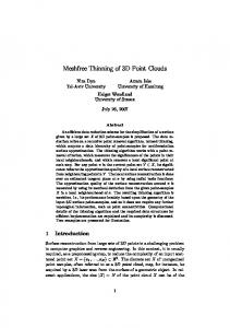
Ncylinder Figure 2. Neighborhood definitions used in this work as the basis for extracting features for a considered 3D point X: cylindrical neighborhoods Nc with different radii (green) and spherical neighborhood Nk,opt formed by an optimal number kopt of nearest neighbors (blue). may be applied where, in addition to the feature vector of the considered 3D point X, the spatial relationship to other neighboring 3D points is considered in order to assign the class label. An approach for a contextual classification of ALS point cloud data has for instance been presented by applying a Conditional Random Field on the basis of cylindrical neighborhoods (Niemeyer et al., 2014), and the respective classification results represent the baseline for the ISPRS benchmark on 3D semantic labeling. 3. METHODOLOGY For each 3D point X to be classified, the proposed framework successively applies three main steps which consist in the recovery of a local neighborhood (Section 3.1), the extraction of geometric features based on those 3D points within the local neighborhood (Section 3.2) and the supervised classification of the derived feature vector (Section 3.3). 3.1

Recovery of Local Neighborhoods

To obtain an appropriate local neighborhood as the basis for feature extraction, we focus on the use of a multi-scale, multi-type neighborhood (Blomley et al., 2016) as e.g. given in Figure 2. The multi-scale, multi-type neighborhood used in the scope of this work comprises four cylindrical neighborhoods Nc with radii of 1m, 2m, 3m and 5m (Niemeyer et al., 2014; Schmidt et al., 2014), and a spherical neighborhood Nk,opt formed by the k closest neighbors, whereby the scale parameter k is derived via eigenentropy-based scale selection (Weinmann et al., 2015a; Weinmann, 2016) and may hence be individual for each 3D point X. 3.2

Extraction of Geometric Features

• Maximum height difference ∆H within the neighborhood • Standard deviation of height values σH within the neighborhood For the spherical neighborhood Nk,opt whose scale parameter has been determined via eigenentropy-based scale selection, we additionally consider the radius R of the considered local neighborhood. Furthermore, we extract covariance features (West et al., 2004; Pauly et al., 2003) which are derived from the normalized eigenvalues λi (i ∈ {1, 2, 3}) of the 3D structure tensor, where λ1 ≥ λ2 ≥ λ3 ≥ 0 and λ1 + λ2 + λ3 = 1: • Linearity: Lλ =

λ1 −λ2 λ1

• Planarity: Pλ =

λ2 −λ3 λ1

• Sphericity: Sλ =

λ3 λ1

• Omnivariance: Oλ = • Anisotropy: Aλ =

√ 3

λ1 λ2 λ3

λ1 −λ3 λ1

• Eigenentropy: Eλ = −λ1 ln (λ1 ) − λ2 ln (λ2 ) − λ3 ln (λ3 ) • Sum of eigenvalues: Σλ = λ1 + λ2 + λ3 • Local surface variation: Cλ =

λ3 λ1 +λ2 +λ3

3.2.2 Shape Distributions: Originally, this type of sampled features has been proposed to describe the shape of a complete object (Osada et al., 2002). The used adaptation of shape distributions to describe geometric properties of the local neighborhood around a considered 3D point X has been presented in (Blomley et al., 2014). Generally, shape distributions are histograms of shape values, which may be derived from random point samples by applying (distance or angular) metrics as shown in Figure 3: • A3: angle between any three random points • D1: distance of one random point from the centroid of all points within the neighborhood • D2: distance between two random points

The derived multi-scale, multi-type neighborhood serves as the basis for extracting features. In the following, we distinguish between two feature types. Shape measures describe features that comprise a single value each, whereby the value specifies one (mathematical) property of the whole set of 3D points within the evaluated local neighborhood (Section 3.2.1). As a consequence, such features are typically interpretable. In contrast, shape distributions are characterized by the fact that each feature is represented by a collection of values e.g. in the form of histograms (Section 3.2.2), where single values are hardly interpretable. Finally, all features are concatenated to a respective feature vector and a subsequent normalization is carried out so that each feature may contribute approximately the same, independent of its unit and its range of values. For more details on the applied normalization, we refer to (Blomley et al., 2016).

• D3: square root of the area spanned by a triangle between three random points • D4: cubic root of the volume spanned by a tetrahedron between four random points Since the histogram counts of randomly sampled shape values within each local neighborhood constitute the feature values, appropriate histogram binning thresholds and a suitable number of random pulls are crucial prerequisites. Following (Blomley et al., 2014), we select 10 histogram bins, i.e. 10 feature values will be produced from each metric, and we perform 255 pulls from the local neighborhood. The binning thresholds of the histogram are estimated by applying the adaptive histogram binning procedure presented in the aforementioned reference.

✓ A3

D1

COG

D3

D2

D4

Figure 3. Visualization of the considered shape distribution metrics: angle between any three random points (A3), distance of one random point from the centroid of all points within the neighborhood (D1), distance between two random points (D2), square root of the area spanned by a triangle between three random points (D3), and cubic root of the volume spanned by a tetrahedron between four random points (D4). 3.3

Class Powerline Low Vegetation Impervious Surfaces Car Fence / Hedge Roof Fac¸ade Shrub Tree P

Supervised Classification of Feature Vectors

For each considered 3D point X, all features are concatenated to a respective feature vector and provided as input for classification. To obtain general conclusions about the suitability of using multi-scale, multi-type neighborhoods as the basis for feature extraction, we involve several classifiers relying on different learning principles. 3.3.1 Nearest Neighbor Classifier: This classifier relies on the principle of instance-based learning, where each feature vector in the test set is directly compared to the feature vectors in the training set and the class label of the most similar training example is assigned. As similarity metric, we use the Euclidean distance. 3.3.2 Linear Discriminant Analysis Classifier: This classifier relies on the principle of probabilistic learning, where the aim is to derive an explicit underlying probabilistic model and infer the most probable class label for each observed feature vector. For this purpose, a multivariate Gaussian distribution is fitted to the given training data, i.e. the parameters of a Gaussian distribution are estimated for each class by parameter fitting. Thereby, the same covariance matrix is assumed for each class and only the means may vary. 3.3.3 Quadratic Discriminant Analysis Classifier: This classifier is very similar to the Linear Discriminant Analysis classifier. The difference consists in the fact that not only the means but also the covariance matrices may vary for different classes. 3.3.4 Random Forest Classifier: This classifier relies on the principle of ensemble learning, where the aim is to strategically combine a set of weak learners to form a single strong learner. More specifically, the combination of decision trees as weak learners is realized in a rather intuitive way via bagging (Breiman, 1996) which focuses on training a weak learner of the same type for different subsets of the training data which are randomly drawn with replacement. Accordingly, the weak learners are all randomly different from each other and, hence, taking the majority vote across the hypotheses of all weak learners results in a generalized and robust hypothesis of a single strong learner (Breiman, 2001).

4. EXPERIMENTAL RESULTS In the following, we briefly describe the involved dataset (Section 4.1) and the conducted experiments (Section 4.2), before presenting the results achieved with our framework (Section 4.3).

Training Set 546 180,850 193,723 4,614 12,070 152,045 27,250 47,605 135,173 753,876

Test Set N/A N/A N/A N/A N/A N/A N/A N/A N/A 411,722

Table 1. Number of 3D points per class. Note that the reference labels are only provided for the training set and not available for the test set. 4.1

Dataset

For evaluating the performance of our framework, we use the Vaihingen dataset (Cramer, 2010) – an airborne laser scanning dataset acquired with a Leica ALS50 system over Vaihingen, a small village in Germany. The acquired data corresponds to areas with small multi-story buildings and many detached buildings surrounded by trees. The Vaihingen dataset has been presented in the scope of the ISPRS Test Project on Urban Classification and 3D Building Reconstruction (Rottensteiner et al., 2012), and it meanwhile serves as benchmark dataset for the ISPRS benchmarks on 2D and 3D semantic labeling. More details about this dataset are provided on the ISPRS webpages1 , where the dataset is also available upon request. In the scope of the ISPRS benchmark on 3D semantic labeling, nine semantic classes have been defined for the Vaihingen dataset, and these classes are given by Powerline, Low Vegetation, Impervious Surfaces, Car, Fence / Hedge, Roof, Fac¸ade, Shrub and Tree. The point-wise reference labels have been determined based on (Niemeyer et al., 2014). The Vaihingen dataset is split into a training set and a test set (see Table 1). The training set is visualized in Figure 1 and contains the spatial XY Z-coordinates, reflectance information, the number of returns and the reference labels. For the test set, only the spatial XY Z-coordinates, reflectance information and the number of returns are provided. 4.2

Experiments

The experiments focus on the use of the presented multi-scale, multi-type neighborhood (Section 3.1) for extracting metrical features given by shape measures and distribution features given by shape distributions (Section 3.2) which, in turn, are concatenated to a feature vector serving as input for a respective classifier (Section 3.3). 1 see http://www2.isprs.org/commissions/comm3/wg4/3dsemantic-labeling.html (Accessed: 11 May 2016)

Metric OA κ MCR

NN 45.07 32.08 38.14

LDA 50.19 38.30 49.09

QDA 38.11 27.66 38.65

RF 41.52 30.28 41.30

Class Powerline Low Vegetation Impervious Surfaces Car Fence / Hedge Roof Fac¸ade Shrub Tree

Table 2. Derived classification results for the NN classifier, the LDA classifier, the QDA classifier and the RF classifier: overall accuracy (OA), Cohen’s kappa coefficient (κ) and mean class recall (MCR). For the training phase, we take into account that an unbalanced distribution of training examples per class might have a detrimental effect on the training process (Chen et al., 2004; Criminisi and Shotton, 2013). Accordingly, we introduce a class re-balancing by randomly sampling the same number of training examples per class to obtain a reduced training set. For our experiments, a reduced training set comprising 10,000 training examples per class has proven to yield results of reasonable quality. Note that this results in a duplication of training examples for those classes represented by less than 10,000 training examples. Additionally, it has to be considered that the training process might also rely on different parameters. Whereas the Nearest Neighbor (NN) classifier, the Linear Discriminant Analysis (LDA) classifier and the Quadratic Discriminant Analysis (QDA) classifier do not require parameter tuning, the Random Forest (RF) classifier involves several parameters (such as the number NT of decision trees to be used for classification, the minimum allowable number nmin of training points for a tree node to be split, the number na of active variables to be used for the test in each tree node, etc.) which have to be selected by the user, e.g. by combining a grid search on a suitable subspace with cross-validation. For the test phase, we use the trained classifiers to assign class labels to those 3D points of the test set. The spatial XY Zcoordinates and the estimated labels have been provided to the organizers of the ISPRS benchmark on 3D semantic labeling who performed the evaluation. As evaluation metrics, we consider the overall accuracy (OA), Cohen’s kappa coefficient (κ) and the mean class recall (MCR). Furthermore, we take into account the class-wise evaluation metrics of recall, precision and F1 -score. 4.3

Results

LDA 89.33 12.37 47.63 28.88 20.44 80.70 51.26 38.39 72.76

QDA 40.33 2.29 69.37 35.03 45.45 35.82 50.94 10.19 58.41

RF 74.33 4.45 54.32 22.11 21.75 56.06 50.53 21.60 66.59

Table 3. Class-wise recall values (in %) corresponding to the classification results provided in Table 2. Class Powerline Low Vegetation Impervious Surfaces Car Fence / Hedge Roof Fac¸ade Shrub Tree

NN 7.61 40.70 74.25 12.65 8.26 47.88 17.47 23.61 49.03

LDA 3.03 53.25 84.98 31.36 13.18 48.63 36.75 28.25 57.46

QDA 1.46 44.43 65.51 6.12 5.35 59.92 16.07 20.91 37.29

RF 0.87 50.58 78.18 13.12 7.75 47.94 19.33 33.62 44.44

Table 4. Class-wise precision values (in %) corresponding to the classification results provided in Table 2. Class Powerline Low Vegetation Impervious Surfaces Car Fence / Hedge Roof Fac¸ade Shrub Tree

NN 13.21 23.79 52.17 12.01 11.41 56.82 23.29 26.86 57.71

LDA 5.85 20.07 61.05 30.07 16.03 60.69 42.81 32.55 64.21

QDA 2.81 4.35 67.39 10.42 9.58 44.84 24.43 13.70 45.52

RF 1.73 8.19 64.10 16.47 11.43 51.68 27.96 26.30 53.30

Table 5. Class-wise F1 -scores (in %) corresponding to the classification results provided in Table 2. 5.1

The classification results obtained with the four considered classifiers are visualized in Figures 4 and 5, and they clearly reveal a different behavior. This also becomes visible when looking at the derived values for different evaluation metrics relying on the whole dataset (see Table 2) or at the derived values for the class-wise evaluation metrics (see Tables 3, 4 and 5). The classification metrics of overall accuracy (OA), Cohen’s kappa coefficient (κ) and mean class recall (MCR) indicate that the Linear Discriminant Analysis (LDA) classifier achieves the best performance (OA = 50.19%, κ = 38.30% and MCR = 49.09%) for our application, and a look on the respective processing times required for training and testing (see Table 6) reveals that using a LDA classifier is also favorable in this regard. Note that the RF classifier is the only one of these classifiers which relies on a parameter tuning, i.e. several parameters have to be determined via a heuristic grid search (here: NT = 2,000, nmin = 1, na = 3).

NN 50.33 16.81 40.21 11.43 18.43 69.88 34.90 31.14 70.12

The Proposed Framework

The main goal of the proposed framework consists in the use of geometric features extracted from multi-scale, multi-type neighborhoods to allow a semantic reasoning on point-level. The use of contextual information or additional non-geometric features is not in the scope of this paper, since we intend to obtain insights on the neighborhoods and the features, both representing important prerequisites for achieving adequate classification results. Our results with relatively low numbers for different evaluation metrics indicate that the Vaihingen dataset with a labeling with respect to nine semantic classes represents a rather challenging dataset when focusing on a 3D semantic labeling. To a certain degree, this might be due to the fact that some classes might not be representatively covered in the training data – e.g. the class Powerline with only 546 given training examples and the class Car with 4,614 given training examples (see Table 1) – which, in turn, yields poor classification results for these classes.

5. DISCUSSION Based on the derived results, we may easily get an impression about the pros and cons of the proposed framework for the classification of ALS point clouds (Section 5.1). To also account for other strategies for a semantic labeling of 3D point clouds, we subsequently provide a more general discussion on the pros and cons of point-wise and segment-wise approaches (Section 5.2).

Furthermore, the derived results indicate that only considering geometric features might not be sufficient for obtaining adequate classification results for all considered classes, since some of these classes might have a quite similar geometric behavior, e.g. the classes Low Vegetation, Fence / Hedge and Shrub. This indeed becomes visible in Figures 4 and 5 where particularly misclassifications among these three classes may be observed for different

Figure 4. Derived classification results for the NN classifier (top left), the LDA classifier (top right), the QDA classifier (bottom left) and the RF classifier (bottom right) when using the same color encoding as in Figure 1 (Powerline: violet; Low Vegetation: yellowish green; Impervious Surfaces: royalblue; Car: cyan; Fence / Hedge: pink; Roof : crimson; Fac¸ade: white; Shrub: gold; Tree: emerald-green). Classifier NN LDA QDA RF

ttrain − 18.41s 12.17s 27.36s

ttest 3.30h 32.62s 97.87s 153.73s

Table 6. Required processing times ttrain for the training process and ttest for the classification of the test set when using the NN classifier, the LDA classifier, the QDA classifier and the RF classifier. Note that there is no training process for the NN classifier, since the induction is delayed to the test phase and quite timeconsuming due to the comparison of each feature vector of the test set with each feature vector in the training set. classifiers. Yet, also the extracted geometric features may not be optimal as some of the neighborhoods used as the basis for feature extraction are relatively large, e.g. the cylindrical neighborhoods with radii of 3m and 5m which have also been used in (Niemeyer et al., 2014; Schmidt et al., 2014). This, in turn, results in misclassifications at particularly those locations where the cylindrical neighborhood includes 3D points associated to the classes Roof and Impervious Surfaces. A closer look on the classification results provided in Figures 4

and 5 also reveals seam effects where borders between roofs and fac¸ades or between fac¸ades and ground are largely categorized into the class Fac¸ade, particularly for the QDA classifier and the RF classifier. Furthermore, the QDA classifier provides the best recognition of Impervious Surfaces, while the classification results are rather poor for the classes Low Vegetation, Fence / Hedge and Shrub. In contrast, the LDA classifier provides a good recognition for the classes Roof and Tree, while problems in the separation between Impervious Surfaces and Roof become visible. 5.2

Point-Wise vs. Segment-Wise Approaches

In the scope of this paper, we focus on a point-wise classification of 3D point clouds, since a consideration on point-level results in simplicity and efficiency. The same features are extracted for all 3D points based on their local neighborhood, and the classifiers are rather intuitive and easy-to-use. Furthermore, the whole process of feature extraction and classification can be highly parallelized. As a result, we efficiently obtain a labeling of reasonable accuracy. Due to the use of standard classifiers for classifying each 3D point based on the respective feature vector, we may expect a slightly noisy appearance of the classified 3D point cloud – which indeed becomes visible in Figures 4 and 5 – since these classifiers do not account for a spatial correlation between class

Figure 5. Derived classification results for the NN classifier (top left), the LDA classifier (top right), the QDA classifier (bottom left) and the RF classifier (bottom right) when using the same color encoding as in Figure 1 (Powerline: violet; Low Vegetation: yellowish green; Impervious Surfaces: royalblue; Car: cyan; Fence / Hedge: pink; Roof : crimson; Fac¸ade: white; Shrub: gold; Tree: emerald-green). labels of neighboring 3D points. Such a spatial correlation could for instance be considered by applying approaches for contextual classification such as Conditional Random Fields which are e.g. used in (Niemeyer et al., 2014; Weinmann et al., 2015b). In contrast, a consideration of 3D point clouds on a segmentlevel certainly relies on the use of an appropriate segmentation approach in order to provide a meaningful partitioning of a 3D point cloud into smaller, connected subsets which correspond to objects of interest or to parts of these (Melzer, 2007; Vosselman, 2013). Due to the complexity of real-world scenes and the objects therein, however, it often remains non-trivial to obtain a reasonable partitioning without either (i) using the result of an initial point-wise classification or (ii) integrating prior knowledge in the form of object models for those objects expected in the scene. Furthermore, it has to be taken into account that a fully generic segmentation typically results in a high computational effort. 6. CONCLUSIONS In this paper, we have presented a framework for semantically labeling 3D point clouds acquired via airborne laser scanning. Our framework relies on the use of complementary types of geometric

features extracted from multi-scale, multi-type neighborhoods as input for a standard classifier. Involving several classifiers with different learning principles, the results derived for a challenging dataset with nine classes indicate that geometric features allow to detect the classes Impervious Surfaces, Roof and Tree – which are characteristic for an urban environment – with an acceptable accuracy. However, there are also classes with a rather similar geometric behavior, e.g. the classes Low Vegetation, Fence / Hedge and Shrub which are not appropriately assigned in the derived classification results. One reason for this has been identified in the fact that some of the neighborhoods used as the basis for feature extraction are relatively large (e.g. the cylindrical neighborhoods with radii of 3m and 5m) and thus cause many misclassifications due to a “smoothing” of details. In future work, we intend to investigate potential sources for improving the classification results. This may include an extension of the presented framework by deriving further features (e.g. from reflectance information, the number of returns, etc.) and/or by considering contextual information inherent in the data. Furthermore, we plan to investigate steps from a semantic labeling of 3D point clouds on point-level to a semantic labeling on objectlevel in order to classify objects of interest and thus allow an object-based scene analysis.

ACKNOWLEDGEMENTS This work was partially supported by the Carl-Zeiss foundation [Nachwuchsf¨orderprogramm 2014]. The Vaihingen dataset was provided by the German Society for Photogrammetry, Remote Sensing and Geoinformation (DGPF) (Cramer, 2010): http://www.ifp.uni-stuttgart.de/dgpf/ DKEP-Allg.html. REFERENCES Blomley, R., Jutzi, B. and Weinmann, M., 2016. Classification of airborne laser scanning data using geometric multi-scale features and different neighbourhood types. In: ISPRS Annals of the Photogrammetry, Remote Sensing and Spatial Information Sciences, Prague, Czech Republic, Vol. III-3, pp. 169–176. Blomley, R., Weinmann, M., Leitloff, J. and Jutzi, B., 2014. Shape distribution features for point cloud analysis – A geometric histogram approach on multiple scales. In: ISPRS Annals of the Photogrammetry, Remote Sensing and Spatial Information Sciences, Z¨urich, Switzerland, Vol. II-3, pp. 9–16. Breiman, L., 1996. Bagging predictors. Machine Learning 24(2), pp. 123–140. Breiman, L., 2001. Random forests. Machine Learning 45(1), pp. 5–32. Brodu, N. and Lague, D., 2012. 3D terrestrial lidar data classification of complex natural scenes using a multi-scale dimensionality criterion: applications in geomorphology. ISPRS Journal of Photogrammetry and Remote Sensing 68, pp. 121–134. Chehata, N., Guo, L. and Mallet, C., 2009. Airborne lidar feature selection for urban classification using random forests. In: The International Archives of the Photogrammetry, Remote Sensing and Spatial Information Sciences, Paris, France, Vol. XXXVIII-3/W8, pp. 207–212. Chen, C., Liaw, A. and Breiman, L., 2004. Using random forest to learn imbalanced data. Technical Report, University of California, Berkeley, USA. Cramer, M., 2010. The DGPF-test on digital airborne camera evaluation – Overview and test design. PFG Photogrammetrie – Fernerkundung – Geoinformation 2 / 2010, pp. 73–82. Criminisi, A. and Shotton, J., 2013. Decision forests for computer vision and medical image analysis. Advances in Computer Vision and Pattern Recognition, Springer, London, UK. Demantk´e, J., Mallet, C., David, N. and Vallet, B., 2011. Dimensionality based scale selection in 3D lidar point clouds. In: The International Archives of the Photogrammetry, Remote Sensing and Spatial Information Sciences, Calgary, Canada, Vol. XXXVIII-5/W12, pp. 97–102. Filin, S. and Pfeifer, N., 2005. Neighborhood systems for airborne laser data. Photogrammetric Engineering & Remote Sensing 71(6), pp. 743– 755. Guo, B., Huang, X., Zhang, F. and Sohn, G., 2015. Classification of airborne laser scanning data using JointBoost. ISPRS Journal of Photogrammetry and Remote Sensing 100, pp. 71–83. Guo, L., Chehata, N., Mallet, C. and Boukir, S., 2011. Relevance of airborne lidar and multispectral image data for urban scene classification using random forests. ISPRS Journal of Photogrammetry and Remote Sensing 66(1), pp. 56–66. Hu, H., Munoz, D., Bagnell, J. A. and Hebert, M., 2013. Efficient 3-D scene analysis from streaming data. In: Proceedings of the IEEE International Conference on Robotics and Automation, Karlsruhe, Germany, pp. 2297–2304. Jutzi, B. and Gross, H., 2009. Nearest neighbour classification on laser point clouds to gain object structures from buildings. In: The International Archives of the Photogrammetry, Remote Sensing and Spatial Information Sciences, Hannover, Germany, Vol. XXXVIII-1-4-7/W5. Khoshelham, K. and Oude Elberink, S. J., 2012. Role of dimensionality reduction in segment-based classification of damaged building roofs in airborne laser scanning data. In: Proceedings of the International Conference on Geographic Object Based Image Analysis, Rio de Janeiro, Brazil, pp. 372–377. Lee, I. and Schenk, T., 2002. Perceptual organization of 3D surface points. In: The International Archives of the Photogrammetry, Remote Sensing and Spatial Information Sciences, Graz, Austria, Vol. XXXIV3A, pp. 193–198.

Linsen, L. and Prautzsch, H., 2001. Local versus global triangulations. In: Proceedings of Eurographics, Manchester, UK, pp. 257–263. Lodha, S. K., Fitzpatrick, D. M. and Helmbold, D. P., 2007. Aerial lidar data classification using AdaBoost. In: Proceedings of the International Conference on 3-D Digital Imaging and Modeling, Montreal, Canada, pp. 435–442. Lodha, S. K., Kreps, E. J., Helmbold, D. P. and Fitzpatrick, D., 2006. Aerial lidar data classification using support vector machines (SVM). In: Proceedings of the International Symposium on 3D Data Processing, Visualization, and Transmission, Chapel Hill, USA, pp. 567–574. Mallet, C., Bretar, F., Roux, M., Soergel, U. and Heipke, C., 2011. Relevance assessment of full-waveform lidar data for urban area classification. ISPRS Journal of Photogrammetry and Remote Sensing 66(6), pp. S71– S84. Melzer, T., 2007. Non-parametric segmentation of ALS point clouds using mean shift. Journal of Applied Geodesy 1(3), pp. 159–170. Mitra, N. J. and Nguyen, A., 2003. Estimating surface normals in noisy point cloud data. In: Proceedings of the Annual Symposium on Computational Geometry, San Diego, USA, pp. 322–328. Niemeyer, J., Rottensteiner, F. and Soergel, U., 2014. Contextual classification of lidar data and building object detection in urban areas. ISPRS Journal of Photogrammetry and Remote Sensing 87, pp. 152–165. Osada, R., Funkhouser, T., Chazelle, B. and Dobkin, D., 2002. Shape distributions. ACM Transactions on Graphics 21(4), pp. 807–832. Pauly, M., Keiser, R. and Gross, M., 2003. Multi-scale feature extraction on point-sampled surfaces. Computer Graphics Forum 22(3), pp. 81–89. Rottensteiner, F., Sohn, G., Jung, J., Gerke, M., Baillard, C., Benitez, S. and Breitkopf, U., 2012. The ISPRS benchmark on urban object classification and 3D building reconstruction. In: ISPRS Annals of the Photogrammetry, Remote Sensing and Spatial Information Sciences, Melbourne, Australia, Vol. I-3, pp. 293–298. Rusu, R. B., Marton, Z. C., Blodow, N. and Beetz, M., 2008. Persistent point feature histograms for 3D point clouds. In: Proceedings of the International Conference on Intelligent Autonomous Systems, BadenBaden, Germany, pp. 119–128. Schmidt, A., Niemeyer, J., Rottensteiner, F. and Soergel, U., 2014. Contextual classification of full waveform lidar data in the Wadden Sea. IEEE Geoscience and Remote Sensing Letters 11(9), pp. 1614–1618. Shapovalov, R., Velizhev, A. and Barinova, O., 2010. Non-associative Markov networks for 3D point cloud classification. In: The International Archives of the Photogrammetry, Remote Sensing and Spatial Information Sciences, Saint-Mand´e, France, Vol. XXXVIII-3A, pp. 103–108. Tombari, F., Salti, S. and Di Stefano, L., 2010. Unique signatures of histograms for local surface description. In: Proceedings of the European Conference on Computer Vision, Heraklion, Greece, Vol. III, pp. 356– 369. Vosselman, G., 2013. Point cloud segmentation for urban scene classification. In: The International Archives of the Photogrammetry, Remote Sensing and Spatial Information Sciences, Antalya, Turkey, Vol. XL-7/W2, pp. 257–262. Vosselman, G., Gorte, B. G. H., Sithole, G. and Rabbani, T., 2004. Recognising structure in laser scanner point clouds. In: The International Archives of the Photogrammetry, Remote Sensing and Spatial Information Sciences, Freiburg, Germany, Vol. XXXVI-8/W2, pp. 33–38. Weinmann, M., 2016. Reconstruction and analysis of 3D scenes – From irregularly distributed 3D points to object classes. Springer, Cham, Switzerland. Weinmann, M., Jutzi, B. and Mallet, C., 2013. Feature relevance assessment for the semantic interpretation of 3D point cloud data. In: ISPRS Annals of the Photogrammetry, Remote Sensing and Spatial Information Sciences, Antalya, Turkey, Vol. II-5/W2, pp. 313–318. Weinmann, M., Jutzi, B., Hinz, S. and Mallet, C., 2015a. Semantic point cloud interpretation based on optimal neighborhoods, relevant features and efficient classifiers. ISPRS Journal of Photogrammetry and Remote Sensing 105, pp. 286–304. Weinmann, M., Schmidt, A., Mallet, C., Hinz, S., Rottensteiner, F. and Jutzi, B., 2015b. Contextual classification of point cloud data by exploiting individual 3D neighborhoods. In: ISPRS Annals of the Photogrammetry, Remote Sensing and Spatial Information Sciences, Munich, Germany, Vol. II-3/W4, pp. 271–278. West, K. F., Webb, B. N., Lersch, J. R., Pothier, S., Triscari, J. M. and Iverson, A. E., 2004. Context-driven automated target detection in 3-D data. Proceedings of SPIE 5426, pp. 133–143. Xu, S., Vosselman, G. and Oude Elberink, S., 2014. Multiple-entity based classification of airborne laser scanning data in urban areas. ISPRS Journal of Photogrammetry and Remote Sensing 88, pp. 1–15.