3D Vision-based Navigation for Indoor Microflyers Antoine Beyeler, Jean-Christophe Zufferey and Dario Floreano
Abstract— Fully autonomous control of ultra-light indoor airplanes has not yet been achieved because of the strong limitations on the kind of sensors that can be embedded making it difficult to obtain good estimations of altitude. We propose to revisit altitude control by considering it as an obstacle avoidance problem and introduce a novel control scheme where the ground and ceiling is avoided based on translatory optic flow, in a way similar to existing vision-based wall avoidance strategies. We show that this strategy is successful at controlling a simulated microflyer without any explicit altitude estimation and using only simple sensors and processing that have already been embedded in an existing 10-gram microflyer. This result is thus a significant step toward autonomous control of indoor flying robots.
I. I NTRODUCTION
other objects like walls instead of the ground. Finally, optic flow estimation are usually impaired with significant amounts of noise since it is dependent on availability of image contrast and subject to the aperture problem [14]. In these conditions, it is very difficult to obtain a metric estimation of the altitude. In this paper, we extend the existing 2D control strategy [2] to 3D by considering pitch control as an obstacle avoidance problem. In the previous scheme, the airplane was controlled into straight trajectories while lateral optic flow due to translation was evaluated. When it reached a fixed threshold, a stereotypic saccade was triggered to avoid walls. Similarly, we propose a control scheme where the airplane flies along straight trajectories in the available volume—that is including climbing and descending trajectories—and to use lateral, dorsal and ventral optic flow to detect close objects to avoid. The avoidance itself is done by horizontal or vertical saccadic maneuvers. This clearly contrasts with traditional approaches where it was attempted to maintain the robot at fixed altitude and then to avoid obstacles within this 2D plane parallel to the ground. In the next section, we describe this novel control architecture. We then describe the physics-based simulation of an existing 10-gram microflyer called MC1 [1] (Fig. 1) that we used to assess the control scheme. Finally, we present the results obtained so far and discuss them.
We aim at developing vision-based controllers for less than 10-gram microflyers [1] in order to achieve fully autonomous flight in indoor environments. Significant advances have been made in this domain over the past decade by using insect-inspired navigation strategies based on optic flow [2]–[5]. Optic flow indeed contains implicit information on surrounding distances to objects due to motion parallax [6]– [8]. Traditional approaches that rely on inertial measurement units (IMU), GPS or active distance sensors are impossible in indoors due to the weight and consumption of these sensors. On the contrary, lightweight cameras, MEMS rate gyros and anemometers have already been successfully embedded in 10-gram airplanes [1]. However, previous studies still showed severe limitations. In particular, altitude control either was inexistent [2] or preliminary and unstable due to the fact that the rotational optic flow generated by pitch rotations was ignored [3]–[5]. A scheme to overcome this problem has been suggested [9], but is unlikely to be directly implementable in the tiny microcontrollers embedded in real microflyers. Finally, a few successful demonstrations of altitude control were made in simulation [10], [11], but the underlying physics of the agents was far too simplified—no inertia and no roll angle required to turn—to be relevant to fixed-wing airplanes. Contrary to airships [12] or slow moving helicopters [13], the dynamics of airplanes require relatively high attitude angles (up to 45◦ ) in order to perform maneuvers like turns, climbs or descents. This means that most of the time, the distance perceived by a downward pointing camera is not the true altitude but a distance that depends on the airplane’s attitude. Additionally, the camera very often sees
A. Sensors and actuators
The authors are with the Laboratory of Intelligent Systems (LIS), Ecole Polytechnique F´ed´erale de Lausanne (EPFL), CH-1015 Lausanne, Switzerland. Email:
[email protected]
Fig. 2 describes the system we plan to control. It is based on the MC1 microflyer [1] and is actuated using two control surfaces—the rudder and the elevator—and a thruster. For
Fig. 1.
Picture of the 10-gram indoor microflyer called MC1 [1].
II. C ONTROL
left FOV 30° α (d)
(b)
(c)
right FOV top FOV
(e) (a) 30°
β (d) (b)
(c)
bottom FOV Fig. 2. Schema of the target airplane. It is based on the MC1 microflyer [1]. The airplane is controlled using its rudder (a), elevator (b) and thruster (c). It is equipped with a yaw and pitch rate gyro (d), an anemometer (e), and a vision system capable of looking left-, right-, up- and downward.
the purpose of this paper, the microflyer is equipped with a vision system capable of measuring longitudinal optic flow at four separate looking directions, on the left, the right, up and down. There is an angle α between the airplane’s main axis and the lateral fields of view, and an angle β for the top and bottom fields of view. Additionally, this microflyer possesses two rate gyros measuring rotation speed about the yaw and pitch axis. They can be used to compensate for spurious optic flow generated by rotations in order to focus on translatory optic flow that alone contains information on distances to neighboring objects. Finally, an anemometer measuring the airspeed is embedded on the airplane. Note that the existing obstacle avoidance scheme already used the left and right optic flow detector and the yaw gyro to control the rudder. B. 3D control scheme Fig. 3 presents a block diagram of the 3D control scheme. The top part concerns the lateral saccadic behavior and is very similar to the previously suggested steering control [2]. Left and right optic flow is compensated using the yaw rate gyro by removing the rotational component and compared to a threshold θH . If these values are under the threshold, the microflyer is forced to fly straight using a proportional regulation based on the yaw rate gyro (with a gain Ky ). As soon as one of the lateral optic flow signals reaches the threshold, a saccade is triggered in the opposite
direction. The saccade duration is linearly modulated using the opposite, non-triggering optic flow value. A high opposite optic flow value means that the microflyer is approaching the wall in a perpendicular way or is flying toward a corner. Both of these situations indeed need a longer saccade to properly move away from the obstacle. On the other hand, if the airplane approaches tangentially to the wall, the opposite optic flow will have a lower value due to the larger distance and the saccade will thus be shorter. The actual saccade is implemented using a series of open-loop commands applied on the rudder and an increment δe to the elevator to compensate for the additional lift needed to turn. Finally, an inhibitory period of length ∆i prevents a new saccade from being triggered immediately after the previous one. The central part of Fig. 3 shows the pitch control scheme, which constitutes the main novelty of our approach by enhancing the 2D steering control to full 3D obstacle avoidance. The control is based on a proportional regulator (with gain Kp ) that controls the pitch rate of the airplane. Normally, the set point is fixed to zero in order to maintain the pitch angle constant and to fly along straight trajectories— either leveled, climbing or descending. When either the top or bottom optic flow signals reach a threshold θV , the set point is modulated to impose a pitch rotation to the plane. The modulation is proportional to the difference of the optic flow signal and the threshold (with a gain Km ). Finally, as illustrated in the bottom part of Fig. 3, the airspeed is simply regulated to a target value vt by a proportional regulator (with gain Kv ) using the signal obtained from the anemometer. It is interesting to note that our control scheme comprises a high-level and low-level part, as shown in Fig. 3. The lowlevel part includes several regulators and the stereotypical yaw saccade. All of these components need to be tuned to the underlying flying platform. On the other hand, the highlevel part is generic and is in principle not dependent on the details of the underlying dynamics. III. S IMULATION Our simulation setup is built upon a custom engine called Enlil1 . It consists of a lightweight implementation of scene graph that uses OpenGL for rendering and the Open Dynamics Engine (ODE)2 for the physics simulation. Inspired on our new microflyer testing arena [1], the simulated environment (Fig. 4) is modeled as a square room of 8×8 (m) with a ground-to-ceiling distance of 3 (m). All the surfaces are textured using synthetic textures made of blurred random checkerboard. The microflyer dynamics model is based on the aerodynamic stability derivatives [15]. These derivatives associate a coefficient for each aerodynamical contribution to each of the 6 forces and moments acting on the airplane and linearly sum 1 Enlil is currently in early development stage. It is publicly available under the GPL license at http://lis.epfl.ch/enlil, including the flight model. 2 http://www.ode.org/
+
right OF (α)
+
Saccade initiation
–
Threshold (θH , ∆i )
trigger direction duration
Series of openloop commands (δe ) Yaw stabilization
yaw gyro
S
P regulator (Ky ) Pitch stabilization
+
pitch gyro
–
+
bottom OF (β)
+
–
Pitch modulation
P regulator (Kp )
+
rudder
elevator pitch control
top OF
Adjustment of set point (θV , Km ) Thrust regulation P regulator (vt , Kv ) high-level control
thrust
airspeed control
anemometer
Fig. 3.
Saccade execution yaw control
left OF
low-level control
Block diagram for the 3D flight control scheme. The parameters of each block are indicated in parenthesis. See text for details.
Fig. 4.
Simulated environment.
them. The forces are then passed to ODE for the kinematics integration. So far, the coefficients have been tuned by hand to reproduce the typical behaviors of the real MC1 [1] when manually controlled. While the model is not yet close enough to the real airplane to be able to easily transfer controllers designed in simulation, the physics is certainly relevant enough for the purpose of this paper. In particular, it displays realistic fixed-wing flight behavior, contrary to the simplified dynamics of agents used in previous implementations of optic-flow-based 3D navigation in simulation [10], [11]. For example, the airplane needs to bank in order to turn. In the future, this will be further improved thanks to ongoing parameter identification experiments in wind tunnel. The vision system is closely modeled after the cameras
available on the MC1. It consists of linear arrays of pixels, whose individual looking directions are separated by a fixed angle, effectively corresponding to a spherical projection. Note that OpenGL only allows for planar projections. For this reason, some post-processing must be applied on OpenGLrendered images in order to obtain spherically projected images. The technique we used for that purpose is essentially a simplified, 1D version of the processing described in [11]. In order to extract optic flow from the images obtained with this camera, we use the 1D version of the image interpolation algorithm (I2A) [16] that has already been successfully used in our microflyers and proved to be easily implementable in 8-bit microcontrollers [1], [2]. Each of the 4 optic flow signals are obtained by applying this algorithm on a 30-pixel image corresponding to each of the fields of view represented in Fig. 2. The signals are then smoothed using a first-order temporal low-pass filter (with a time constant of 200 (ms)).
The other sensors we used in the simulation corresponds to the MC1’s anemometer, yaw and pitch rate gyro. So far, no effort have been made to model these sensors in detail. For the rate gyros, we directly used the rotation speed as provided by ODE. Similarly, the translation speed along the robot main axis was used for the anemometer. Given the quality of the signal provided by modern MEMS rate gyros, this approximation is quite reasonable. However, in the future, a more elaborate model for the anemometer may be necessary since this sensor is more likely to suffer from perturbations and noise.
TABLE I
8
C ONTROL PARAMETERS Value 45◦ 55◦ 30 (◦ /s) 28 (◦ /s) 0.4 (s) 0.3 1.0 0.8 2.0 30% 1.5 (m/s)
7 6 5 y (m)
Parameter α β θH θV ∆i Ky Kp Km Kv δe vt
4 3 2 1 0
IV. R ESULTS
3 A video showing an example of flight is available at http: //lis.epfl.ch/research/projects/microflyers/videos/ mc1 3d simul.mpg.
2
4 x (m)
6
8 1
z (m)
3 2
0.5 1 0 0
2
4 x, y (m)
6
8
Fig. 5. Room occupancy averaged on the 20 test flights. The top graph shows a top view. The bottom graph shows an average of both lateral views.
3 2 z (m)
Using the simulation environment described above, we implemented the control strategy presented in section II. As a first step, all the parameters, including the gains, the thresholds, the saccade series of commands and camera viewing directions, were tuned by hand in order to achieve good flight performances. The obtained values are listed in table I. While the obtained controller showed a reasonable reliability, the manual tuning is probably less than perfect, but this preliminary experiment is intended as a proof of concept of 3D obstacle avoidance control for less than 10gram microflyers. In the future, we plan to use optimization techniques like genetic algorithms. At this stage, out of 20 test flights3 , we obtained an average of 90 (sec) before crash, with best flights lasting more than 5 (min). Each flight included on average 30 lateral saccades, with a maximum of 115 for the longest flight, where the distance flown was about 600 (m). Fig. 5 represents the normalized probability of finding the airplane at any position in the available volume, based on all of the 20 test flights. The top graph shows a view from above, while the bottom graph shows an averaged view from both side. It shows that the microflyer visits all the available surface when seen from above. However, there is a clear bias toward positions at low altitude, as discussed below. Fig. 6 shows a 20-second sample of flight data, and the corresponding trajectory is represented in Fig. 7. The two top graphs show the evolution of the translatory optic flow estimation for the left and right fields of view. Note that the values for the left optic flow are negative. The threshold is also indicated, and one can clearly see how saccades (represented by the gray bars) are triggered as soon as one signal crosses the threshold. The second graph shows the yaw rate of the microflyer which is indicative of the lateral behavior of the airplane. Between saccades it is regulated to a null value, and raises during saccades, either positively or negatively depending on the direction of the saccade. It is interesting to note how the optic flow signals are perturbed during saccades.
0
0 1
2 4
0 8
6 6
4
2
0
8
y (m)
x (m) Fig. 7. Sample trajectory corresponding to the flight data shown in Fig. 6.
The third graph of Fig. 6 shows the evolution of the top (positive) and bottom (negative) translatory optic flow signals, while the fourth shows the altitude of the airplane. Clearly, the microflyer follows straight climbing or descending trajectories between saccades. Very often, the pitch angle is brought down during saccade maneuvers. This is due to the high energy consumption of such maneuvers where a significant amount of lift is used to make the airplane turn instead of counteracting gravity. This explains the bias toward low altitude that was observed in Fig. 5. It also shows
50 0 left optic flow (°/s) –50
right optic flow (°/s)
yaw control
200
yaw rate (°/s)
0 –200
50 0 bottom optic flow (°/s) –50
top optic flow (°/s)
pitch control
altitude (m)
3 2 1 0
speed (m/s)
airspeed control
2 1 0 0
2
4
6
8
10 time (s)
12
14
16
18
20
Fig. 6. Flight data for 20 seconds taken in the middle of a 5-minute flight. The gray bars represent lateral saccades. Note that the optic flow values are the low-pass filtered translatory component.
that the airplane sometimes reaches low altitude between saccades. In this case, the bottom optic flow value increases (negatively) largely past the threshold which leads to a pitch up maneuver. Again, note how top and bottom optic flow signals are perturbed during saccades, although it does not perturb significantly the maneuver execution. Finally, the last graph shows the forward speed of the airplane. The velocity is most of the time very close to the 1.5 (m/s) target, and only slightly decreases for short periods of time during the most ample saccades. V. D ISCUSSION It is interesting to note that the behavior of the airplane shares some similarities with the common fly, that are capable of flying along very complex 3D trajectories that exploit all the available volume [17], [18]. They do not seem to do so by strictly regulating their altitude but rather by avoiding ground and ceiling just as well as walls and other obstacles, using only the sensory modalities of their compound eyes [19], [20], the gyroscopic information provided by their halteres [21] and, probably, the airspeed as sensed by hairs and antennae [22]. Both the strategy and the sensors used to achieve it are similar to our microflyer. There are also some interesting comments to make on the saccadic nature of the control scheme. The reason for using a stereotypic lateral saccade is to cope with the complex dynamics of the turn. In order to steer, microflyers that are not equipped with ailerons use the rudder that first generates side-slip, which in turn makes it roll due to aerodynamical effects. It is finally the roll angle and the corresponding inclination of the lift vector that generate the turn. As
discussed in the previous section, stereotypical saccades are also useful since optic flow measurements during turns are heavily disturbed by the high roll angles and fast rotations, as shown in Fig. 6. On the contrary, such a stereotypic mechanism is not needed for the pitch saccades because the dynamics is significantly simpler. The elevator directly controls the pitch rate of the airplane without affecting the other axes. The results we presented in the previous section show a possible way for a simplification of the design. Since the plane is clearly biased toward low altitude positions, due to the pitching down occurring during saccades, it is likely that the control strategy could be simplified to require only the bottom optic flow camera without the top one. This could be done by slightly trimming the airplane nose-down, in order to avoid long lasting climbing trajectories. This would significantly reduce the complexity of the required vision system and would further ease the implementation of the controller to real microflyers. While our preliminary experiments have demonstrated the viability of our 3D obstacle avoidance scheme, it still has some limitations at the moment. In particular, there are some situations where the microflyer touches the walls or the ground, often leading to a crash. This happens mostly when the airplane flies straight toward the intersection of two walls and the ceiling or ground, which are the most difficult situations. Moreover, all the control parameters were tuned by hand so far, and it is likely that they are not yet optimal in terms of performance and robustness. Finally, the model for both the flight dynamics, the rate gyros and the anemometer are relatively simple and not yet realistic enough to hope
for a successful transfer of controllers from the simulation environment to the real MC1. VI. C ONCLUSION AND FUTURE WORK In this paper, we presented a scheme for full 3D control of autonomous indoor microflyers based on optic flow that can successfully be used to provide the airplane with autonomy using only simple sensors and processing that have already been embedded in an existing platform. Contrary to previous studies that aimed at precisely controlling the altitude, we suggested a different approach where the airplane avoids the ground and ceiling as well as walls without trying to maintain a precise altitude. Our simulations show that this approach is successful at maintaining a microflyer airborne in a simple indoor environment. To cope with the limitations highlighted in the previous section, future work will include several improvements. First, we will use genetic algorithms to optimize our design— including control parameters and camera layout—in a more systematic way. Also, to enhance the usefulness of the results we obtain in simulation, we will improve our flight model of the MC1 by running wind tunnel experiments with the real platform. Embedded sensors will also undergo a more thorough modeling, including noise and dynamic response. Finally, the realism of the simulation will also be improved by introducing better lighting and more realistic textures. All these improvements will ease the transfer of our control scheme and its future refinements to the real microflyer. ACKNOWLEDGMENTS The authors wish to thank Okuary Osechas for his help in the flight model design. This project is supported by the Swiss National Science Foundation, grant 200021-105545/1. R EFERENCES [1] J.-C. Zufferey, A. Klaptocz, A. Beyeler, J. Nicoud, and D. Floreano, “A 10-gram microflyer for vision-based indoor navigation,” in Submitted to IEEE/RSJ International Conference on Intelligent Robots and Systems, 2006. [2] J.-C. Zufferey and D. Floreano, “Fly-inspired visual steering of an ultralight indoor aircraft,” IEEE Transactions on Robotics, vol. 22, pp. 137–146, 2006. [3] W. Green, P. Oh, K. Sevcik, and G. Barrows, “Autonomous landing for indoor flying robots using optic flow,” in ASME International Mechanical Engineering Congress and Exposition, vol. 2, 2003, pp. 1347–1352.
[4] G. Barrows, C. Neely, and K. Miller, “Optic flow sensors for MAV navigation,” in Fixed and Flapping Wing Aerodynamics for Micro Air Vehicle Applications, ser. Progress in Astronautics and Aeronautics, T. J. Mueller, Ed. AIAA, 2001, vol. 195, pp. 557–574. [5] J. Chahl, M. Srinivasan, and H. Zhang, “Landing strategies in honeybees and applications to uninhabited airborne vehicles,” The International Journal of Robotics Research, vol. 23, no. 2, pp. 101– 110, 2004. [6] T. Whiteside and G. Samuel, “Blur zone,” Nature, vol. 225, pp. 94–95, 1970. [7] J. Koenderink and A. van Doorn, “Facts on optic flow,” Biological Cybernetics, vol. 56, pp. 247–254, 1987. [8] J.-C. Zufferey, “Bio-inspired vision-based flying robots,” Ph.D. dissertation, Swiss Federal Institute of Technology in Lausanne (EPFL), 2005. [9] A. Beyeler, C. Mattiussi, J.-C. Zufferey, and D. Floreano, “Visionbased altitude and pitch estimation for ultra-light indoor aircraft,” in IEEE International Conference on Robotics and Automation ICRA ’06, 2006, pp. 2836–2841. [10] T. Neumann, S. Huber, and H. B¨ulthoff, “Minimalistic approach to 3d obstacle avoidance behavior from simulated evolution,” in Proceedings of the 7th International Conference on Artificial Neural Networks (ICANN), ser. Lecture Notes in Computer Science, vol. 1327. Springer-Verlag, 1997, pp. 715–720. [11] T. Neumann and H. B¨ulthoff, “Behavior-oriented vision for biomimetic flight control,” in Proceedings of the EPSRC/BBSRC International Workshop on Biologically Inspired Robotics, 2002, pp. 196–203. [12] J. Zufferey, A. Guanella, A. Beyeler, and D. Floreano, “Flying over the reality gap: From simulated to real indoor airships,” Autonomous Robots, 2006, to appear. [13] S. Bouabdallah, P. Murrieri, and R. Siegwart, “Towards autonomous indoor micro vtol,” Autonomous Robots, vol. 18, no. 2, pp. 171–183, 2005. [14] H. Mallot, Computational Vision: Information Processing in Perception and Visual Behavior. The MIT Press, 2000. [15] J. Cooke, M. Zyda, D. Pratt, and R. McGhee, “Npsnet: Flight simulation dynamic modeling using quaternions,” Presence: Teleoperators and Virtual Environments, vol. 1, no. 4, pp. 404–420, 1992. [16] M. Srinivasan, “An image-interpolation technique for the computation of optic flow and egomotion,” Biological Cybernetics, vol. 71, pp. 401–416, 1994. [17] C. Schilstra and J. van Hateren, “Blowfly flight and optic flow. I. thorax kinematics and flight dynamics,” Journal of Experimental Biology, vol. 202, pp. 1481–1490, 1999. [18] J. van Hateren and C. Schilstra, “Blowfly flight and optic flow. II. head movements during flight,” Journal of Experimental Biology, vol. 202, pp. 1491–1500, 1999. [19] N. Franceschini, “Sampling of the visual environment by the compound eye of the fly: Fundamentals and applications,” in Photoreceptor Optics, A. W. Snyder and R. Menzel, Eds. Springer, Berlin, 1975, pp. 98–125. [20] M. Land, “Visual acuity in insects,” Annual Review of Entomology, vol. 42, pp. 147–177, 1997. [21] G. Nalbach and R. Hengstenberg, “The halteres of the blowfly calliphora. II. Three-dimensional organization of compensatory reactions to real and simulated rotations,” Journal of Comparative Physiology A, vol. 175, no. 6, pp. 695–708, 1994. [22] R. Dudley, The Biomechanics of Insect Flight: Form, Function, Evolution. Princeton University Press, 2000.