4 QR Factorization - Applied Mathematics

4 4.1

QR Factorization Reduced vs. Full QR

Consider A ∈ Cm×n with m ≥ n. The reduced QR factorization of A is of the form ˆ R, ˆ A=Q ˆ ∈ Cm×n with orthonormal columns and R ˆ ∈ Cn×n an upper triangular matrix where Q ˆ such that R(j, j) 6= 0, j = 1, . . . , n. ˆ provides an orthonormal basis for range(A), i.e., the columns of As with the SVD Q ˆ In fact, we have range(A) = range(Q). ˆ A are linear combinations of the columns of Q. ˆ ˆ ˆ ˆ This is true since Ax = QRx = Qy for some y so that range(A) ⊆ range(Q). Moreover, ˆ since we can write AR ˆ −1 = Q ˆ because R ˆ is upper triangular with range(Q) ⊆ range(A) −1 ˆ ˆ nonzero diagonal elements. (Now we have Qx = AR x = Ay for some y.) Note that any partial set of columns satisfy the same property, i.e., span{a1 , . . . , aj } = span{q 1 , . . . , q j },

j = 1, . . . , n.

In order to obtain the full QR factorization we proceed as with the SVD and extend ˆ to a unitary matrix Q. Then A = QR with unitary Q ∈ Cm×m and upper triangular Q R ∈ Cm×n . Note that (since m ≥ n) the last m − n rows of R will be zero.

4.2

QR Factorization via Gram-Schmidt

We start by formally writing down the QR factorization A = QR as a1 r11 a2 − r12 q 1 a2 = q 1 r12 + q 2 r22 =⇒ q 2 = r22 .. .. . . P an − ni=1 rin q i an = q 1 r1n + q 2 r2n + . . . + q n rnn =⇒ q n = rnn a1 = q 1 r11 =⇒ q 1 =

(14) (15) (16) (17)

Note that in these formulas the columns aj of A are given and we want to determine the columns q j of Q and entries rij of R such that Q is orthonormal, i.e., q ∗i q j = δij ,

(18)

R is upper triangular and A = QR. The latter two conditions are already reflected in the formulas above. Using (14) in the orthogonality condition (18) we get q ∗1 q 1 =

a∗1 a1 =1 2 r11

so that r11 =

p

a∗1 a1 = ka1 k2 . 36

Note that we arbitrarily chose the positive square root here (so that the factorization becomes unique). Next, the orthogonality condition (18) gives us q ∗1 q 2 = 0 q ∗2 q 2 = 1. Now we apply (15) to the first of these two conditions. Then q ∗1 q 2 =

q ∗1 a2 − r12 q ∗1 q 1 = 0. r22

Since we ensured q ∗1 q 1 = 1 in the previous step, the numerator yields r12 = q ∗1 a2 so that a2 − (q ∗1 a2 )q 1 q2 = . r22 To find r22 we normalize, i.e., demand that q ∗2 q 2 = 1 or equivalently kq 2 k2 = 1. This immediately gives r22 = ka2 − (q ∗1 a2 )q 1 k2 . To fully understand how the algorithm proceeds we add one more step (for n = 3). Now we have three orthogonality conditions: q ∗1 q 3 = 0 q ∗2 q 3 = 0 q ∗3 q 3 = 1. The first of these conditions together with (17) for n = 3 yields q ∗1 q 3 =

q ∗1 a3 − r13 q ∗1 q 1 − r23 q ∗1 q 2 =0 r33

so that r13 = q ∗1 a3 due to the orthonormality of columns q 1 and q 2 . Similarly, the second orthogonality condition together with (17) for n = 3 yields q ∗2 q 3 =

q ∗2 a3 − r13 q ∗2 q 1 − r23 q ∗2 q 2 =0 r33

so that r23 = q ∗2 a3 . Together this gives us q3 =

a3 − (q ∗1 a3 )q 1 − (q ∗2 a3 )q 2 r33

and the last unknown, r33 , is determined by normalization, i.e., r33 = ka3 − (q ∗1 a3 )q 1 − (q ∗2 a3 )q 2 k2 .

37

In general we can formulate the following algorithm: rij vj

= q ∗i aj = aj −

(i 6= j) j−1 X

rij q i

i=1

rjj qj

= kv j k2 vj = rjj

We can compute the reduced QR factorization with the following (somewhat more practical and almost Matlab implementation of the) classical Gram-Schmidt algorithm. Algorithm (Classical Gram-Schmidt) for j = 1 : n v j = aj for i = 1 : (j − 1) rij = q ∗i aj v j = v j − rij q i end rjj = kv j k2 q j = v j /rjj end Remark The classical Gram-Schmidt algorithm is not ideal for numerical calculations since it is known to be unstable. Note that, by construction, the Gram-Schmidt algorithm yields an existence proof for the QR factorization. Theorem 4.1 Let A ∈ Cm×n with m ≥ n. Then A has a QR factorization. Moreover, ˆR ˆ with rjj > 0 is unique. if A is of full rank (n), then the reduced factorization A = Q Example We compute the QR factorization for the matrix   1 2 0 A =  0 1 1 . 1 0 1 

 1 √ First v 1 = a1 =  0  and r11 = kv 1 k = 2. This gives us 1   1 v1 1   0 . q1 = =√ kv 1 k 2 1

38

Next, v 2 = a2 − (q ∗1 a2 ) q 1 | {z } =r12

    √ 2 1 1 2 =  1  − √  0  =  1 . 2 1 0 −1 



This calculation required that r12 =

√2 2

=

√

2. Moreover, r22 = kv 2 k =

√

3 and



 1 1 v2 = √  1 . q2 = kv 2 k 3 −1 In the third iteration we have v 3 = a3 − (q ∗1 a3 ) q 1 − (q ∗2 a3 ) q 2 | {z } | {z } =r13

from which we first compute r13 =

√1 2

=r23

and r23 = 0. This gives us

     −1 0 1 1 1 1 v3 =  1  − √ √  0  − 0 =  2  . 2 2 2 1 1 1 

√

Finally, r33 = kv 3 k =

6 2

and 

 −1 1 v3 = √  2 . q3 = kv 3 k 6 1 Collecting all of the information we end up with   1 1 −1 √

2

 Q= 0

√1 2

4.3

√

3 √1 3 −1 √ 3

√

6 √2 6 √1 6

 

 √

√ 2 2 √  and R =  0 3 0 0

√1 2



 0 .

√

6 2

An Application of the QR Factorization

Consider solution of the linear system Ax = b with A ∈ Cm×m nonsingular. Since Ax = b

⇐⇒

QRx = b

⇐⇒

Rx = Q∗ b,

where the last equation holds since Q is unitary, we can proceed as follows: ˆR ˆ in this case). 1. Compute A = QR (which is the same as A = Q 2. Compute y = Q∗ b. 39

3. Solve the upper triangular Rx = y We will have more applications for the QR factorization later in the context of least squares problems. Remark The QR factorization (if implemented properly) yields a very stable method for solving Ax = b. However, it is about twice as costly as Gauss elimination (or A = LU ). In fact, the QR factorization can also be applied to rectangular systems and it is the basis of Matlab’s backslash matrix division operator. We will discuss Matlab examples in a later section.

4.4

Modified Gram-Schmidt

The classical Gram-Schmidt algorithm is based on projections of the form vj

= aj −

= aj −

j−1 X i=1 j−1 X

rij q i (q ∗i aj )q i .

i=1

Note that this means we are performing a sequence of vector projections. The starting point for the modified Gram-Schmidt algorithm is to rewrite one step of the classical Gram-Schmidt algorithm as a single matrix projection, i.e., vj

= aj −

j−1 X

(q ∗i aj )q i

i=1

= aj −

j−1 X

(q i q ∗i )aj

i=1

ˆ j−1 Q ˆ ∗ aj = aj − Q j−1   ˆ j−1 Q ˆ ∗j−1 aj , = I −Q | {z } =Pj

ˆ j−1 = [q 1 q 2 . . . q j−1 ] is the matrix formed by the column vectors q i , i = where Q 1, . . . , j − 1. In order to obtain the modified Gram-Schmidt algorithm we require the following observation that the single projection Pj can also be viewed as a series of complementary projections onto the individual columns q i , i.e., ˆ j−1 = [q 1 q 2 . . . q j−1 ] a matrix with orthonorˆ j−1 Q ˆ ∗ with Q Lemma 4.2 If Pj = I − Q j−1 mal columns, then j−1 Y Pj = P⊥qi . i=1

40

Proof First we remember that ˆ ∗j−1 = I − ˆ j−1 Q Pj = I − Q

j−1 X

q i q ∗i

i=1

and that the complementary projector is defined as P⊥qi = I − q i q ∗i . Therefore, we need to show that I−

j−1 X

q i q ∗i =

i=1

j−1 Y

(I − q i q ∗i ) .

i=1

This is done by induction. For j = 1 the sum and the product are empty and the statement holds by the convention that an empty sum is zero and an empty product is the identity, i.e., P1 = I. Now we step from j − 1 to j. First j Y

(I −

q i q ∗i )

=

i=1

j−1 Y

(I − q i q ∗i ) I − q j q ∗j




i=1

=

I−

j−1 X

! q i q ∗i

I − q j q ∗j




i=1

by the induction hypothesis. Expanding the right-hand side yields I−

j−1 X

q i q ∗i − q j q ∗j +

i=1

j−1 X i=1

q i q ∗i q j q ∗j |{z} =0

so that the claim is proved. Summarizing the discussion thus far, a single step in the Gram-Schmidt algorithm can be written as v j = P⊥qj−1 P⊥qj−2 . . . P⊥q1 aj , or – more algorithmically: v j = aj for i = 1 : (j − 1) v j = v j − q i q ∗i v j end For the final modified Gram-Schmidt algorithm the projections are arranged differently, i.e., P⊥qi is applied to all v j with j > i. This leads to

41

Algorithm (Modified Gram-Schmidt) for i = 1 : n v i = ai end for i = 1 : n rii = kv i k2 qi =

vi rii

for j = (i + 1) : n rij = q ∗i v j v j = v j − rij q i end end We can compare the operations count, i.e., the number of basic arithmetic operations (‘+’,‘-’,‘*’,‘/’), of the two algorithms. We give only a rough estimate (exact counts will be part of the homework). Assuming vectors of length m, for the classical GramSchmidt roughly 4m operations are performed inside the innermost loop (actually m multiplications and m−1 additions for the inner product, and m multiplications and m subtractions for the formula in the second line). Thus, the operations count is roughly j−1 n X X

4m =

j=1 i=1

n X

(j − 1)4m ≈ 4m

j=1

n X j=1

j = 4m

n(n + 1) ≈ 2mn2 . 2

The innermost loop of the modified Gram-Schmidt algorithm consists formally of exactly the same operations, i.e., requires also roughly 4m operations. Thus its operation count is !   n X n n n X X X n(n + 1) 2 2 4m = (n − i)4m = 4m n − i = 4m n − ≈ 2mn2 . 2 i=1 j=i+1

i=1

i=1

Thus, the operations count for the two algorithms is the same. In fact, mathematically, the two algorithms can be shown to be identical. However, we will learn later that the modified Gram-Schmidt algorithm is to be preferred due to its better numerical stability (see Section 4.6).

4.5

Gram-Schmidt as Triangular Orthogonalization

One can view the modified Gram-Schmidt algorithm (applied to the entire matrix A) as ˆ AR1 R2 . . . Rn = Q, (19)

42

where R1 , . . . , Rn are upper triangular matrices. For  1/r11 −r12 /r11 −r13 /r11  0 1 0   0 0 1 R1 =   ..  .

R2

   =   

··· ··· ..

.

−r1m /r11 0 0 .. .

···

0

1 0 ··· 0 1/r22 −r23 /r22 · · · 0 0 1 .. .. . . 0 ··· 0

0 −r2m /r22 0 .. .

0 

example,     ,  

1       

1

and so on. ˆ Thus we are applying triangular transformation matrices to A to obtain a matrix Q with orthonormal columns. We refer to this approach as triangular orthogonalization. Since the inverse of an upper triangular matrix is again an upper triangular matrix, and the product of two upper triangular matrices is also upper triangular, we can think ˆ −1 . Thus, the (modified) of the product R1 R2 . . . Rn in (19) in terms of a matrix R Gram-Schmidt algorithm yields a reduced QR factorization ˆR ˆ A=Q of A.

4.6

Stability of CGS vs. MGS in Matlab

The following discussion is taken from [Trefethen/Bau] and illustrated by the Matlab code GramSchmidt.m (whose supporting routines clgs.m and mgs.m are part of a computer assignment). We create a random matrix A ∈ R80×80 by selecting singular values 12 , 14 , . . . , 2180 and generating A = U ΣV ∗ with the help of (orthonormal) matrices U and V whose entries are normally distributed random numbers (using the Matlab command randn). Then we compute the QR factorization A = QR using both the classical and modified Gram-Schmidt algorithms. The program then plots the diagonal elements of R together with the singular values. First we note that 80 X A= σi ui v Ti i=1

so that aj = A(:, j) =

80 X

σi ui vji .

i=1

Next, V is a normally distributed random unitary matrix, and therefore the entries in one of its columns satisfy 1 |vji | ≈ √ ≈ 0.1. 80 43

Now from the (classical) Gram-Schmidt algorithm we know that r11 = ka1 k2 = k

80 X

σ1 v1i ui k2 .

i=1

Since the singular values were chosen to decrease exponentially only the first one really matters, i.e., 1 1 r11 ≈ kσ1 v11 u1 k2 = σ1 v11 ≈ √ 2 80 (since ku1 k2 = 1). Similar arguments result in the general relationship 1 rjj ≈ √ σj 80 (the latter of which we know). The plot produced by GramSchmidt.m shows how accurately the diagonal elements of R are computed. We can observe that the classical √ Gram-Schmidt algorithm is stable up to σj ≈ eps (where eps is the machine epsilon), whereas the modified Gram-Schmidt method is stable all the way up to σj ≈ eps. Remark In spite of the superior stability of the modified Gram-Schmidt algorithm it still may not produce “good” orthogonality. Househoulder reflections – studied in the next chapter – work better (see an example in [Trefethen/Bau]).

4.7

Householder Triangularization

Recall that we interpreted the Gram-Schmidt algorithm as triangular orthogonalization ˆ AR1 R2 . . . Rn = Q leading to the reduced QR factorization of an m × n matrix A. Now we will consider an alternative approach to computing the (full) QR factorization corresponding to orthogonal triangularization: Qn Qn−1 . . . Q2 Q1 A = R, where the matrices Qj are unitary. The idea here is to design matrices Q1 , . . . , Qn such that A is successively transformed to upper triangular form, i.e.,     x x x x x x  x x x   0 x x     A=  x x x  −→ Q1 A =  0 x x  x x x 0 x x     x x x x x x  0 x x     −→ Q3 Q2 Q1 A =  0 x x  , −→ Q2 Q1 A =   0 0 x   0 0 x  0 0 x 0 0 0 44

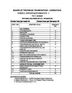
where x stands for a generally nonzero entry. From this we note that Qk needs to operate on rows k : m and not change the first k − 1 rows and columns. Therefore it will be of the form   Ik−1 O Qk = , O F where Ik−1 is a (k − 1) × (k − 1) identity matrix and F has the effect that F x = kxke1 in order to introduce zeros in the lower part of column k. We will call F a Householder reflector. Graphically, we can use either a rotation (Givens rotation) or a reflection about the bisector of x and e1 to transform x to kxke1 . Recall from an earlier homework assignment that given a projector P , then (I −2P ) is also a projector. In fact, (I −2P ) is a reflector. Therefore, if we choose v = kxke1 −x ∗ and define P = vv v ∗ v , then vv ∗ F = I − 2P = I − 2 ∗ v v is our desired Householder reflector. Since it is easy to see that F is Hermitian, so is Qk . Note that F x can be computed as   vv ∗ vv ∗ v∗x Fx = I − 2 ∗ x = x − 2 ∗ x = x − 2v ∗ . v v v v v v |{z} |{z} matrix scalar In fact, we have two choices for the reflection F x: v + = −x + sign(x(1))kxke1 and v − = −x − sign(x(1))kxke1 . Here x(1) denotes the first component of the vector x. These choices are illustrated in Figure 4. A numerically more stable algorithm

Figure 4: Graphical interpretation of Householder reflections. (that will avoid cancellation of significant digits) will be guaranteed by choosing that reflection which moves x further. Therefore we pick v = x + sign(x(1))kxke1 , which is the same (except for orientation) as v − . The resulting algorithm is

45

Algorithm (Householder QR) for k = 1 : n

(sum over columns)

x = A(k : m, k) v k = x + sign(x(1))kxk2 e1 v k = v k /kv k k2 A(k : m, k : n) = A(k : m, k : n) − 2v k (v ∗k A(k : m, k : n)) end Note that the statement in the last line of the algorithm performs the reflection simultaneously for all remaining columns of the matrix A. On completion of this algorithm the matrix A contains the matrix R of the QR factorization, and the vectors v 1 , . . . , v n are the reflection vectors. They will be used to calculate matrix-vector products of the form Qx and Q∗ b later on. The matrix Q itself is not output. It can be constructed by computing special matrix-vector products Qx with x = e1 , . . . , en . Example We apply Householder reflection to x = [2, 1, 2]T . First we compute v = x + sign(x(1))kxk2 e1       5 1 2      1 + 3 0 = 1 . = 2 0 2 ∗

Next we form F x = x − 2v vv∗xv . To this end we note that v ∗ x = 15 and v ∗ v = 30. Thus       2 5 −3 15 F x =  1  23  1  =  0 . 30 2 2 0 This vector contains the desired zero. For many applications only products of the form Q∗ b or Qx are needed. For example, if we want to solve the linear system Ax = b then we can do this with the QR factorization by first computing y = Q∗ b and then solving Rx = y. Therefore, we list the respective algorithms for these two types of matrix vector products. For the first algorithm we need to remember that Qn . . . Q2 Q1 A = R, {z } | =Q∗

so that we can apply exactly the same steps that were applied to the matrix A in the Householder QR algorithm: Algorithm (Compute Q∗ b) for k = 1 : n 46

b(k : m) = b(k : m) − 2v k (v ∗k b(k : m)) end For the second algorithm we use Q = Q1 Q2 . . . Qn (since Q∗i = Qi ), so that the following algorithm simply performs the reflection operations in reverse order: Algorithm (Compute Qx) for k = n : −1 : 1 x(k : m) = x(k : m) − 2v k (v ∗k x(k : m)) end The operations counts for the three algorithms listed above are
Householder QR: O 2mn2 − 32 n3 Q∗ b, Qx: O(mn)

47